Abstract
Forest fuels are the core element of fire management; each fuel component plays an important role in fire behavior. Therefore, accurate determination of their characteristics and spatial distribution is crucial. This paper introduces a novel method for mapping the spatial distribution of litter and duff fuel loads using data collected by unmanned aerial vehicles. The approach leverages a very high-resolution multispectral data analysis within a machine learning framework to achieve precise and detailed results. A set of vegetation indices and texture metrics derived from the multispectral data, optimized by a “Variable Selection Using Random Forests” (VSURF) algorithm, were used to train random forest (RF) models, enabling the modeling of high-resolution maps of litter and duff fuel loads. A field campaign to measure fuel loads was conducted in the mixed forest of the natural protected area of “Sierra de Quila”, Jalisco, Mexico, to measure fuel loads and obtain field reference data for calibration and validation purposes. The results revealed moderate determination coefficients between observed and predicted fuel loads with R2 = 0.32, RMSE = 0.53 Mg/ha for litter and R2 = 0.38, RMSE = 13.14 Mg/ha for duff fuel loads, both with significant p-values of 0.018 and 0.015 for litter and duff fuel loads, respectively. Moreover, the relative root mean squared errors were 33.75% for litter and 27.71% for duff fuel loads, with a relative bias of less than 5% for litter and less than 20% for duff fuel loads. The spatial distribution of the litter and duff fuel loads was coherent with the structure of the vegetation, despite the high complexity of the study area. Our modeling approach allows us to estimate the continuous high-resolution spatial distribution of litter and duff fuel loads, aligned with their ecological context, which dictates their dynamics and spatial variability. The method achieved acceptable accuracy in monitoring litter and duff fuel loads, providing researchers and forest managers with timely data to expedite decision-making in fire and forest fuel management.
1. Introduction
Forest fires are simultaneously considered agents of disturbance and ecosystem shapers. Their occurrence increases every year due to various factors, with climate change being one of the most important [1]. A trend in their increment has been identified in recent years, associated with more frequent heat waves and prolonged drought periods [2]. However, this trend is not uniformly distributed globally. Some areas present precipitation and humidity increases, favoring the accumulation of forest fuels [3]. Future projections indicate climate as a highly relevant factor in global fire trends, even surpassing the current human influence on both their ignition and extinction [4]. Moreover, according to IPCC forecasts (2024) [5], climatic conditions will favor the presence and spread of fires, particularly large fires around the world [6]. Forest fire implications involve a wide range of ecological, economic, and social impacts [7,8]. Globally, wildfire suppression has been widely implemented [9]. However, in many ecosystems this approach can lead to counterproductive outcomes, resulting in an excessive buildup of forest fuels leading to more severe wildfires, especially in the context of climate change [10]. Therefore, accurate spatial information on forest fuels is crucial for effective fire planning and management [11,12,13].
Some countries, such as Mexico, have recently implemented forest fire management policies for which forest fuels are considered a core element [14]. Forest fuels comprise dead organic matter and living vegetation that can potentially burn when exposed to an ignition source [15]. Fuel load is the most common concept used to describe the amount of fuel per unit area, and it is calculated for each component of the fuel complex [16], including dead organic matter (such as down woody debris [DWD], litter, and duff) and living vegetation (like herbs, shrubs, and trees). Understanding fuel load distributions across landscapes is essential for assessing fire behavior, predicting fire spread, and planning effective fire management strategies. Fuels are usually stratified according to their vertical position (e.g., ground, surface, and canopy fuels) [17]. Due to their dissimilar characteristics, each fuel stratum typically results in different types of fires: ground fires primarily burn duff fuels; surface fires spread through litter, DWD, and understory vegetation; and crown fires mainly spread through canopy fuels.
Accurate descriptions of forest fuels are important for fire risk reductions. Canopy fuels direct crown fires, often causing severe effects that require human intervention [18]. Nevertheless, the majority of the world’s wildfires originate from surface fuels. Most ecosystems in the world contain surface fuel litter, herbs, shrubs, and down woody material. Litter can dry quickly and is highly flammable, allowing for the fast spread of fire [15]. When surface fuels are exposed to an ignition source, the spread of fire can be very high and can eventually ignite ground and canopy fuels [19]. The most common ground fuel is duff, which is usually present as a result of surface fuel decomposition [20]. Duff provides a slow spread of fire, but high intensity that remains latent for a long time, causing severe consequences in ecosystems [21]. Forest fuel stratifications have been useful for feeding fuel classification and fire behavior modeling systems [22,23]. However, for high-resolution forest fuel management, each fuel component must be considered in an independent way [15].
Developing high-resolution, accurate maps of the different fuel components remains a challenge [24]. Because forest fuels interact dynamically with the environment, a shift in approach is necessary to enhance estimations within a natural ecological context. The complex biophysical processes occurring in ecosystems play a pivotal role in determining the dynamics of fuel production, deposition, and decomposition, further complicating the mapping process [15].
The environment plays a crucial role in shaping and interacting with forest fuels. Chávez-Durán et al. (2022) [25] developed a method that utilizes environmental variables as a framework for structuring sampling designs to characterize forest fuels. This method identifies areas with similar conditions, referred as to homogeneous response areas (HRAs), using as variables altitude, precipitation, vegetation index, and forest canopy height. For instance, in “Sierra de Quila” Jalisco, Mexico, four HRAs have been identified, each characterized by unique environmental conditions. In “Sierra de Quila” HRA1, for instance, litter is the prominent surface fuel due to low solar radiation transmission through the canopy, a result of the area’s high forest canopy height and dense vegetation. This limited sunlight inhibits understory growth, leading to sparse understory vegetation [26,27]. Additionally, the decomposition of litter in the HRA1 produces abundant duff, especially under deciduous canopies due to their mass loss characteristics [20].
Employing ecological frameworks is valuable for structuring sampling designs for field measurements, which are essential for creating high-resolution fuel load maps. Traditional fieldwork is notoriously labor-intensive, but the process of obtaining accurate measurements for litter and duff fuel loads requires even greater attention. Beyond the fieldwork itself, samples must be transported, classified, dried, weighed, and stored in the laboratory, making the entire process both costly and time-consuming [21,28]. As a result, the most common strategy involves using small, limited sampling plots with minimal remeasurements [29,30].
Remote sensing offers a sound alternative to complement fieldwork and laboratory processes. They promise an alternative for incorporating spatial variability to produce detailed maps of fuel load distribution, as well as for creating and updating fuel load maps across extensive areas [31,32]. However, the literature indicates that remote sensing approaches are primarily used for estimating fuels in the upper strata, i.e., canopy fuels, while other fuel components are often under-represented [33,34,35]. Furthermore, a trend towards the estimation of discrete fuel class maps has been identified, summarizing fuel loads by types or by models [36,37]. This approach to mapping fuel classes is very useful, especially for regional planning purposes. However, under the current global scenario, these maps need to be complemented with continuous detailed and accurate maps of fuel loads, suitable for fire management [38]. However, remote sensing techniques for high-resolution mapping surface and ground fuel loads are still in the early stages of development.
Several studies have reported significant variations in accuracy, influenced by factors such as the study area, sensors used, and the scale of the research [39,40]. Labenski et al. (2023) [41] utilized airborne light detection and ranging (LiDAR) in conjunction with multispectral data from Sentinel-2, employing random forest (RF) regressions to quantify surface fuels. On the other hand, Li et al. (2021) [42] utilized terrestrial LiDAR data and linear logarithmic regression models to estimate surface fuels. However, despite LiDAR’s advantages, its use remains expensive and the availability of high-density LiDAR sensors is still low. Nevertheless, Keane (2015) [15] argued that forest canopy significantly influences the characteristics of fuels beneath it, by affecting their production, deposition, and decomposition. As a result, forest fuel loads below tree canopy cover can be estimated using high-resolution images.
Technological advances, including the use of unmanned aerial vehicles (UAVs) [43], have led to the development of platforms capable of carrying multiple sensor types. UAVs provide the ability to capture high-resolution images with temporal flexibility and reliability [44]. Despite these capabilities, the use of UAV technology for the high-resolution estimation of surface and ground fuels has been poorly documented [45].
The aim of this paper was to develop a method for mapping the spatial distribution of surface and ground fuel loads, specifically litter and duff, using field georeferenced data, high-resolution multispectral imagery, and machine learning techniques. The underlying hypothesis was that machine learning techniques can find relationships between the upper canopy observed by UAV sensors and field measurements of surface and ground fuel loads providing accurate and efficient mapping of the high-resolution spatial distribution of litter and duff fuel loads. The approach aims to produce detailed and reliable fuel load maps that reflect their variability as a result of their ecological context, thereby assisting researchers and forest managers in making timely and informed decisions regarding fire and forest fuel management. The integration of high-resolution imagery and machine learning, such as random forest models, could improve the way ground and surface fuel loads are assessed, leading to more accurate predictions of fire behavior and improved forest management practices.
2. Materials and Methods
2.1. Study Area
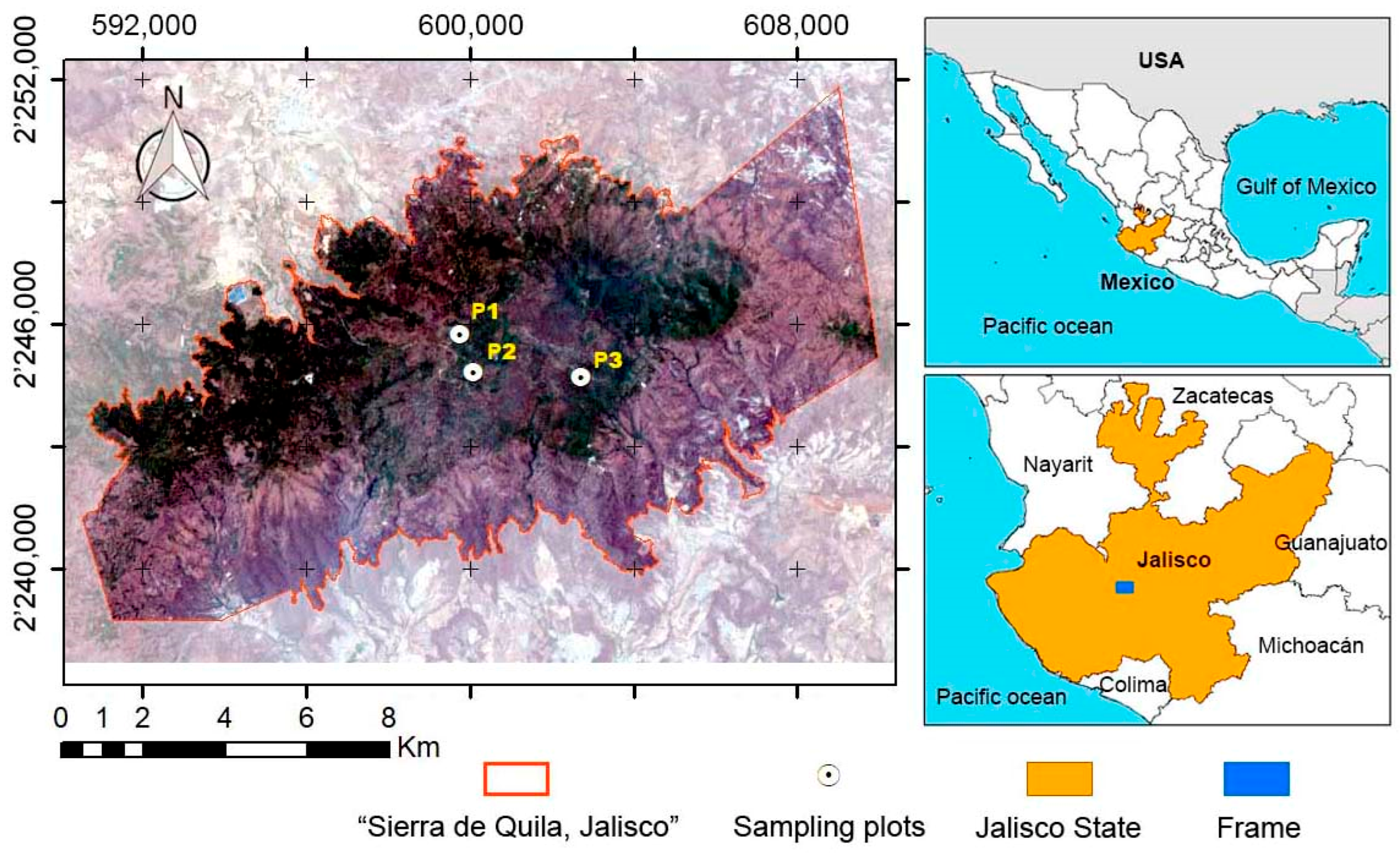
The study was carried out in the natural protected area “Sierra de Quila,” Jalisco, Mexico, located at bounding coordinates 20°14.65′ N to 20°21.67′ N and -103°56.79′ W to -104°7.98′ W (Figure 1), within an altitudinal range spanning from 1357 to 2544 m asl. The area comprises 15,192.50 ha, with vegetation mainly dominated by temperate forests, composed of Pinus and Quercus genus, with Pinus douglasiana and Quercus resinosa as the most abundant species. The potential fire regime is characterized by frequent, low-severity surface fires [46,47]. However, due to fire suppression, the potential fire regime has been altered and devastating crown fires have occurred, with strong implications for both ecosystem and forest fighters [48]. Previous studies classified the area into four HRAs [25] and the spatial distribution of canopy fuel loads (CFLs) has been studied [32].

Figure 1.
Image depicting the study area location and showing sampling plots. The projection coordinate system used is Universal Transverse Mercator Zone 13 North (UTM 13N).
2.2. Data and Materials Description
The estimation of the litter and duff fuel load spatial distribution comprised three stages: data collection, processing, and mapping. The data collection stage involved: (1) direct field measurements of fuel loads using permanent sampling plots, and (2) the acquisition of UAVs imagery. The processing stage involved fuel load estimates which were derived from field measurements and integrated with UAV metrics in a machine learning framework. Finally, the mapping stage involved the application of trained RF algorithms to estimate litter and duff fuel loads from remote sensing data (Figure 2).
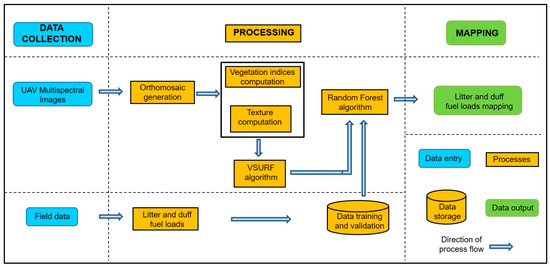
Figure 2.
Flowchart for estimating the spatial distribution of litter and duff fuel loads using variable selection with random forests (VSURF).
2.2.1. Field Data
The field data collection was carried out in May 2022. Three square sampling permanent plots of 1 ha (100 × 100 m) each were established in the study area. The plot corners were delineated with 2 cm precision, using Ruide Total Station RTS-833, georeferenced with a Topcon GR-5 Global Navigation Satellite System (GNSS). The plot coordinates were referenced to the Universal Transverse Mercator, Zone 13 North (UTM 13N) (Figure 1). In each plot, 25 subplots 400 m2 (20 × 20 m) were established using a Sokkisha TM10E theodolite (Figure 3A). Within each subplot, four nanoplots of 0.09 m2 each (0.30 × 0.30 m) were established (Figure 3B) and litter and duff were collected within each one. This setup resulted in a total of 300 observations for each type of fuel.
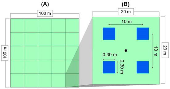
Figure 3.
Sampling plots for field data. (A) One-hectare sampling plot divided into 400 m2 (20 × 20 m) subplots. (B) A subplot showing nanoplots of 0.09 m2 (0.30 × 0.30 m).
The depth of each layer was recorded using Truper® measuring tape (Truper, Mexico City, Mexico). After the depth measurement, the forest fuels from the nanoplots were carefully collected and transferred into plastic bags for transportation to the laboratory (Figure 4A). In the laboratory, the samples were sorted into categories such as duff, Pinus leaves, Quercus leaves, and other materials (e.g., seeds, flowers, and tree barks) (Figure 4B). Each sample was then weighed, dried at 70 °C until a constant weight was achieved, and recorded to ensure accurate measurement [21].

Figure 4.
Field data collection and laboratory process. (A) Litter and duff material collection in situ. (B) Sample classification in laboratory.
The fuel load variables collected in the field were averaged at the subplot level (400 m2) to establish the reference values. Descriptive statistics were then applied as part of the exploratory data analysis. To assess the differences among the plots, the non-parametric Kruskal–Wallis test was employed, as the assumption of homoscedasticity was not met according to the Levene test (p-value < 0.05) [49,50]. For subsequent pairwise comparisons, the Wilcoxon–Mann–Whitney test was used [51].
Previous studies have highlighted the significance of spatial autocorrelation in achieving high-resolution estimates of fuel loads [28,52]. To ensure the assumption of sample independence, Moran’s index (MI) was applied to assess the spatial distribution of litter and duff. The mean values for each fuel component at the subplot level (400 m2) and their spatial coordinates were used to identify the distribution patterns, following the approach outlined in Equation (1) [53].
where is Moran’s index; is the number of observations; is the sum of weights , is the difference of fuel loads in position with respect to its mean , and is the difference of attribute in position with respect to its mean
2.2.2. Remote Sensing Data and Multispectral Analysis
Remote sensing data were collected in September 2022 using a Sensefly Ebee® UAV (AgEagle Aerial Systems Inc., Wichita, KS, USA) equipped with a Parrot Sequoia+® multispectral camera (Parrot, Paris, France). Spectral information was recorded in four bands: green (530–570 nm), red (640–680 nm), red edge (730–740 nm), and near-infrared (770–810 nm). The UAV was flown at a height of 212 m above the ground, resulting in a spatial resolution of 20 cm. Before each flight, a target calibration panel was used to produce images radiometrically corrected [54]. In each 1 ha plot, 25 images were captured with 80% forward overlap and 60% side overlap. For all flights, ground control points (GCPs) were established to correct the georeferencing of images, and flight plans were created using eMotion 3.5.0® software and grid flight missions [55].
The data were processed using Agisoft Metashape 1.6.4 software, which enables the generation of orthomosaics by spectral calibration data and the structure-from-motion (SfM) algorithm [56]. The internal and relative orientation of individual images was determined based on their metadata spatial reference, ensuring the accurate integration of the imagery. Subsequently, the relative coordinates were transformed into absolute coordinates using GCPs, achieving horizontal and vertical average RMSE values of less than 0.50 m and 0.80 m, respectively. The results were exported as multispectral orthomosaics with their original spatial resolution [57].
The multispectral orthomosaics were used to compute twelve vegetation indices, as described in Chávez-Durán et al. (2024) [32]. They comprise: the normalized difference vegetation index (NDVI); soil adjusted vegetation index (SAVI); modified soil adjusted vegetation index (MSAVI); 2-band enhanced vegetation index (EVI2); difference vegetation index (DVI); green normalized vegetation index (GNDVI); green ratio vegetation index (GRVI); green difference index (GDI); green red difference index (GRDI); red edge normalized difference vegetation index (NDVIre); red edge simple ratio (SRre); and Datt4. These vegetation indices provided detailed spectral information related to vegetation con-dition and cover [58,59].
Moreover, eight textures metrics for each spectral band (Table 1) were derived from 273 the spectral orthomosaics. Texture bands were used to estimate the local spatial variation [60], using the “gray level co-occurrence matrix” (GLCM) which is one of the most efficient and widely used texture estimation methods. GLCM makes it possible to obtain the texture information contained in an image based on the spatial dependencies of the pixel values within a kernel, describing the frequency of individual pairs of values in a window, to estimate the spatial variation of the gray levels [61]. A kernel of 5 × 5 pixels was used to compute different texture metrics such as mean, variance, homogeneity, contrast, dissimilarity, entropy, second moment, and correlation.

Table 1.
Equations used to estimate texture indicators using gray level co-occurrence matrix (GLCM) from Haralick et al. (1973) [62]. Number of distinct gray levels in the quantized image (); ()th entry in a normalized gray-tone spatial dependence matrix (); th entry in the marginal-probability matrix obtained by summing the rows and columns of ( and ); and means and standard deviations of and (, , , ).
2.2.3. Litter and Duff Fuel Load Spatial Distribution
The spatial distribution of the litter and duff fuel loads was estimated using random forest (RF) models, one for each fuel component. RF is a highly effective machine learning algorithm that employs regression techniques through bagging and random subspace methods [63,64]. The metrics from the subplots were pooled and then split into training (70% of the sample) and validation (30% of the sample) datasets. The litter and duff fuel load reference values served as the response variable; to optimize the selection of explanatory variables and avoid collinearity, the “variable selection using random forests” (VSURF) algorithm was used. VSURF is an algorithm included as an R library that makes it possible to select explanatory variables. A two-stage strategy was implemented based on the ranking of the explanatory variables through random forests permutation. The first stage produced a subset of important variables including some redundancy but with potential for interpretation purposes. Based on the score of importance, the second stage resulted in a smaller subset of important variables, seeking to avoid redundancy and focusing more closely on the prediction objective [65]. The importance of each explanatory variable was assessed using the mean decrease accuracy method [66]. The algorithm was calibrated and implemented using the “randomForest, raster and sf” libraires [67,68,69] available in R-project 4.4.0 [70]. The 95% confidence interval for each predicted fuel was computed using bootstrapping pairs [71,72].
The models’ performance was assessed using independent validation data, employing the R2 coefficient, root mean squared error (RMSE) and relative root mean squared error (rRMSE) [73]. In addition, both absolute and relative biases in fuel loads were calculated. Absolute bias was used to assess the performance of the RF-trained model on individual plots, while relative bias enabled comparisons between the plots [74]. These assessments were conducted according to Equations (2) and (3).
where, and correspond to the absolute and relative bias, respectively; is the estimated fuel load for each subplot and is the fuel load observed from the field data.
Statistical analyses were conducted using the following R libraries: “readr, northest, car, FactoMineR, ranger and ggplot2” [75,76,77,78,79,80], available in R-project 4.4.0 [70].
3. Results
3.1. Field Data
Litter fuel loads showed mean values (95% confidence interval) of 1.62 ± 0.14 Mg/ha for P1, 1.89 ± 0.34 Mg/ha for P2, and 1.19 ± 0.20 Mg/ha for P3, with significant statistical differences among the plots as indicated by the Kruskal–Wallis test: H(2) = 14.89, p = 0.0006. According to Wilcoxon–Mann–Whitney test, the litter fuel loads in P1 and P2 were statistically different from P3 with p-value < 0.05. Pinus leaves accounted for 64.27% of the total litter fuel load, Quercus leaves for 21.29%, and others fuel materials for 14.44%. The duff fuel load showed mean values of 54.84 ± 8.83 Mg/ha for P1, 54.58 ± 11.39 Mg/ha for P2 and 50.36 ± 7.88 Mg/ha for P3; there were no significant statistical differences among the plots according to the Kruskal–Wallis test: H(2) = 0.64, p = 0.73. Moreover, the Moran’s index analysis showed that both litter and duff fuel loads were distributed randomly, showing no spatial autocorrelation. For litter, the MI values were as follows: MIP1 = 0.23, MIP2 = 0.23 and MIP3 = 0.10. For duff, MI values were: MIP1 = 0.00, MIP2 = 0.23 and MIP3 = 0.04. All the MI values had a p-value > 0.05, indicating a lack of significant spatial autocorrelation.
3.2. Litter and Duff Fuel Load Spatial Distribution
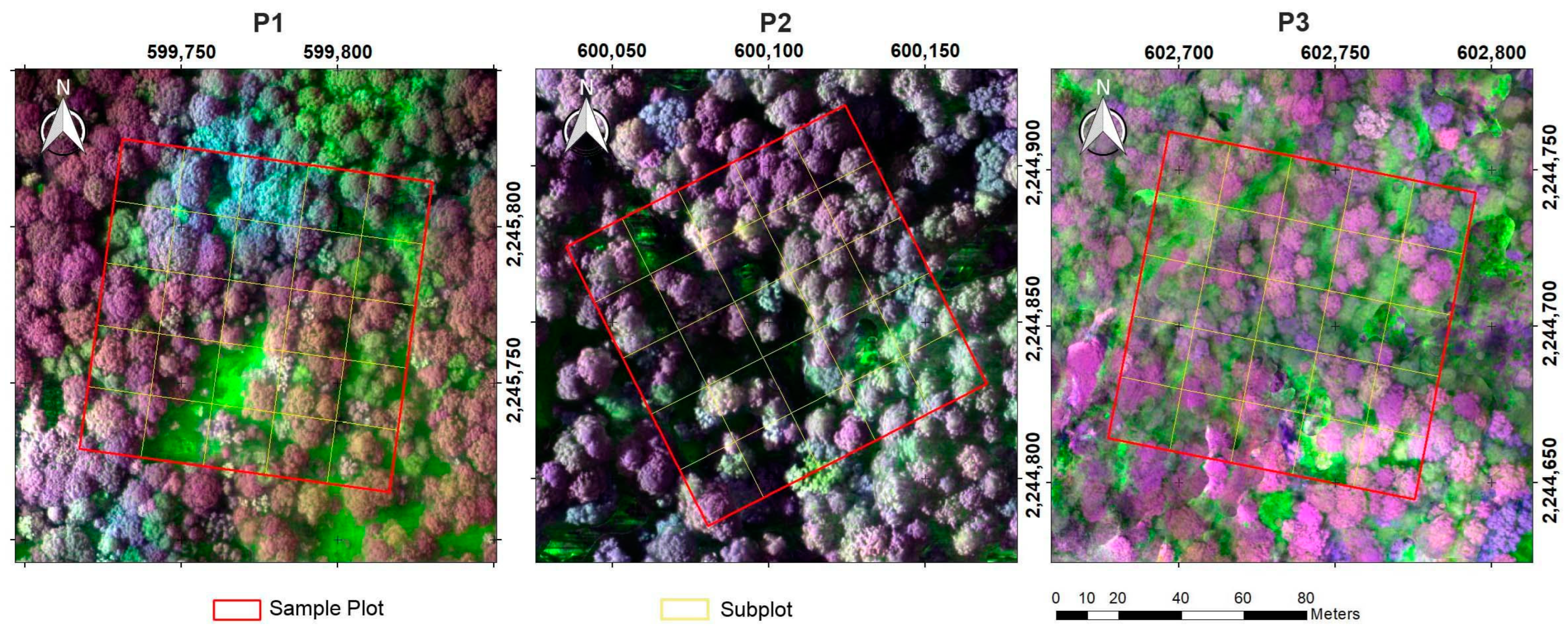
As a result of digital photogrammetry, a set of raw multispectral orthomosaics was obtained (Figure 5), followed by vegetation indices and texture bands. The VSURF algorithm identified the following uncorrelated potential explanatory variables, with a percentage increase of mean squared error in parentheses according to Liaw et al. (2020) [67]. For the litter fuel loads, the variables were GNDVI (5.15), green band homogeneity texture (2.94), red band homogeneity texture (1.32), NDVI (1.03), and green band variance texture (0.55). For the duff fuel loads, the identified variables were the red edge band homogeneity texture (5.00), green band second moment texture (3.49), GRVI (3.42), Datt4 (2.69), red edge band contrast texture (2.66), and NDVIre (0.50) (Appendix A).

Figure 5.
Multispectral orthomosaics for P1, P2, and P3 from the Parrot Sequoia sensor. False-color composition: Green, red, and red edge bands.
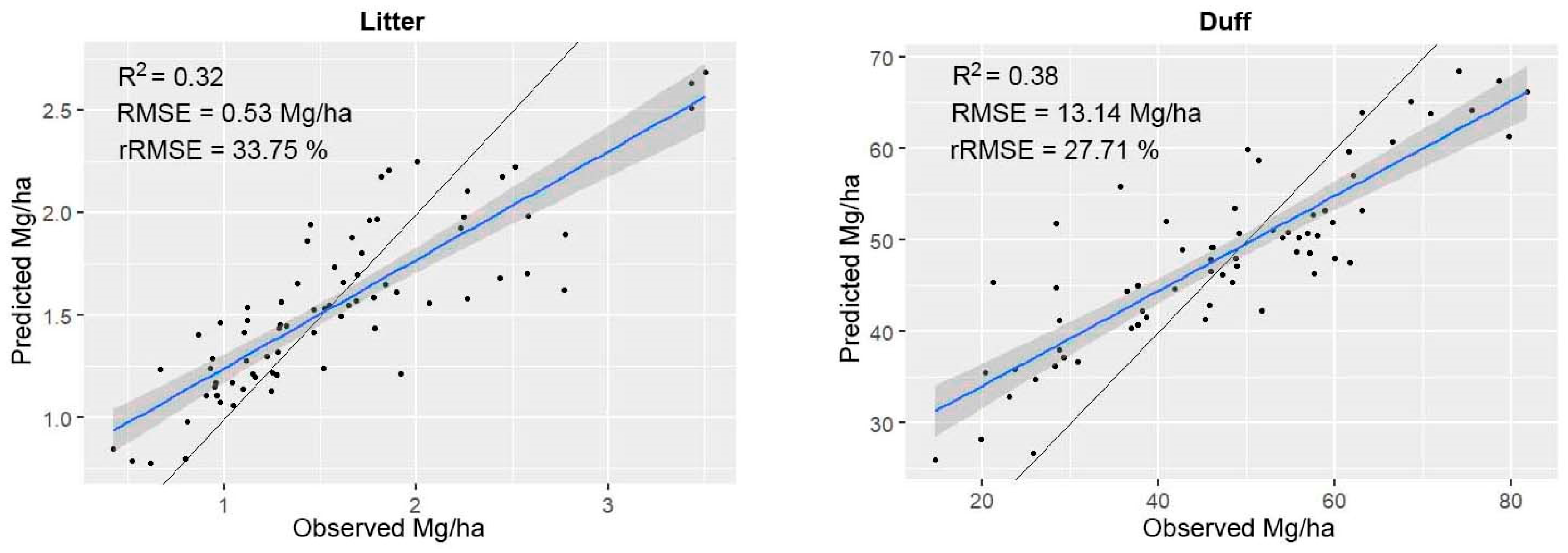
The data validation revealed that models based on remote sensing analysis achieved R2 = 0.32, p-value = 0.018, RMSE = 0.53 Mg/ha for litter and R2 = 0.38, p-value = 0.015, RMSE = 13.14 Mg/ha for duff fuel loads (Figure 6). Furthermore, rRMSE was 33.75% for litter and 27.71% for duff, while the mean relative bias was less than 5% for litter and less than 20% for duff (Table 2).
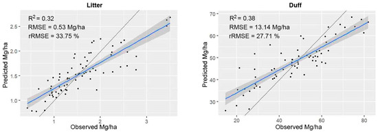
Figure 6.
Predicted vs. observed litter (left) and duff (right) fuel loads. The blue solid line represents the trend line and the shadowed area the 95% confidence interval. The black solid represents the 1:1 line.

Table 2.
Accuracy of litter and duff fuel loads among plots. Absolute bias (Biasabs) and relative bias (Biasrel).
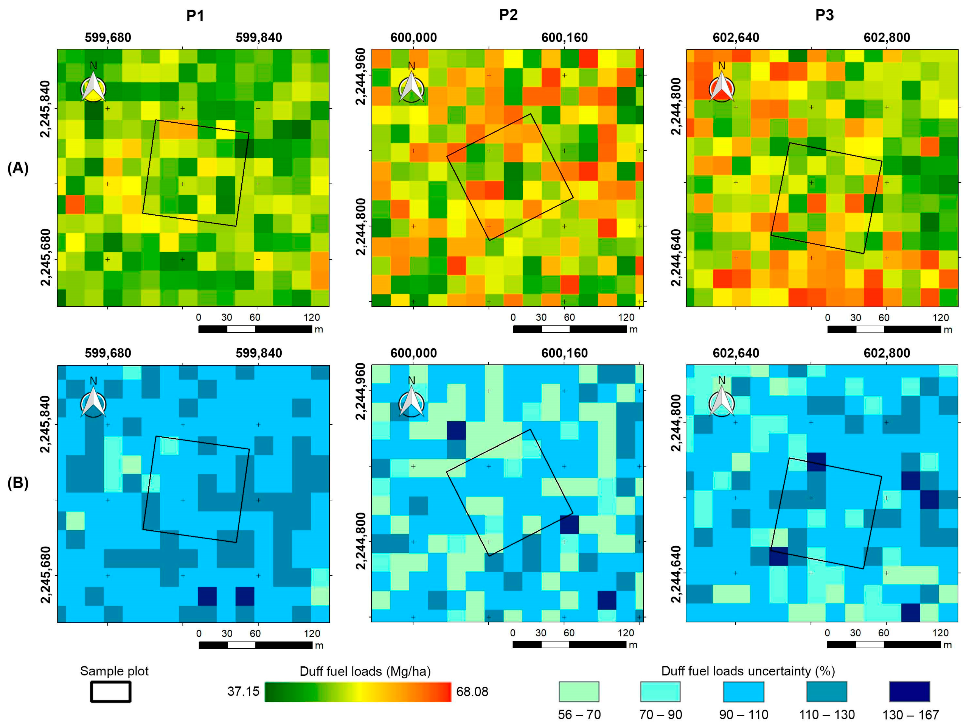
The mean values for the spatial distribution of the litter fuel loads based on the remote sensing data were 1.67, 1.81 and 1.18 Mg/ha for P1, P2, and P3, respectively; for the duff fuel loads, the mean values were: 49.51, 46.38, and 48.00 Mg/ha for P1, P2, and P3, respectively. Additionally, the highest relative uncertainties were associated with the lower values, specifically less than 1.00 Mg/ha for litter and less than 30 Mg/ha for duff fuel loads (Figure 7 and Figure 8).
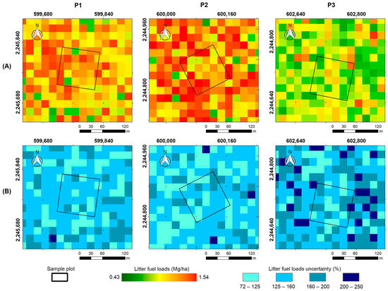
Figure 7.
Litter fuel load spatial distribution. P1, P2, and P3 are 1 ha sampling plots. (A) Litter fuel loads (Mg/ha); (B) Litter fuel load uncertainty (%).
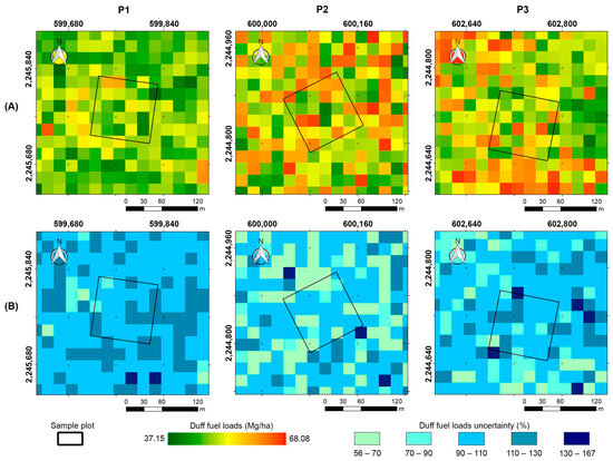
Figure 8.
Duff fuel load spatial distribution. P1, P2, and P3 are 1 ha sampling plots. (A) Duff fuel loads (Mg/ha); (B) Duff fuel loads uncertainty (%).
4. Discussion
4.1. Field Data
The results from the spatial autocorrelation analysis indicate that litter and duff fuel loads are randomly distributed, showing high variability even at short distances. This finding aligns with the results reported by Chávez-Durán et al. (2021) [28], who also found no spatial autocorrelation for litter and duff fuel loads, with differences greater than 100 Mg/ha in samples separated by less than 80 m. Although their study was in “Sierra de Quila”, the sampling plot was in another HRA with different environmental conditions. Ulrich et al. (2014) [81] similarly observed that, at high resolution, vegetation exhibits significant heterogeneity due to the interplay of chemical and physical soil properties with abiotic environmental conditions through the water balance [82]. In our study, the high-resolution data analysis revealed similarly high levels of heterogeneity. These results can be attributed to the significant influence of the vegetation canopy on the characteristics of litter and duff fuel loads [15]. Therefore, our study highlights the importance of conducting high-resolution studies to accurately capture local variability in litter and duff fuel loads, which is essential for understanding the intricate ecological processes occurring within smaller spatial extents.
Litter serves as the primary source of highly flammable and continuous fuel. Our values were lower than those reported by Chávez-Durán et al. (2021) [28], who observed mean values of 17.95 Mg/ha for litter fuel loads. In our study, the majority of the litter fuel loads were derived from Pinus leaves. Chávez-Durán et al. (2024) [32] found that Pinus trees exhibited the highest CFLs values, contributing over 70% in each plot. They also recorded the highest values of other structural variables such as basal area, tree height, and vegetation cover, within the same 1-hectare permanent sample plots in the “Sierra de Quila”. These characteristics explain the significant contribution of Pinus leaves to the total litter fuel loads. Moreover, the limited solar radiation penetrating the canopy results in fewer saplings, herbs, and bushes [26,27]. Consequently, litter becomes the most important surface fuel load, playing a critical role in driving the spread of surface fires [15].
Duff fuels showed the highest fuel loads in our study, with values exceeding those reported by Chávez-Durán et al. (2021) [28], who recorded mean values of 33.12 Mg/ha. Nevertheless, unlike their study, the field data used in our study were collected from the HRA with the highest values of average annual precipitation. Duff is formed from the decomposition of litter through biophysical processes [15]. According to Kwon et al. (2021) [83], in mixed forests, the forest floor accumulates leaf litter from a variety of tree species, which may differ in terms of the timing, quantity, and quality of litter production, as well as in decomposition rates. Factors such as structural stability, chemical properties, and environment conditions are predominant in leaf litter decomposition, leading to varying degrees of decomposition [84]. For practical purposes, most studies treat duff as a single component [22].
Pérez-Suárez et al. (2011) [20] found that rainfall explained 97% of litter mass loss in a mixed forest in central Mexico, with the Pinus genus showing a slower rate of leaf litter mass loss due to its highly significant lignified leaf tissue. In contrast, the Quercus genus showed a greater mass loss, which is attributed to its higher concentration of soluble compounds and lower lignin content. Therefore, in our study, the duff fuel loads were primarily composed of Pinus leaves that remained on the floor for an extended period.
4.2. Litter and Duff Fuel Load Spatial Distribution
Vegetation indices and textures derived from high-resolution UAV multispectral data allowed for an accurate estimation of the litter and duff fuel loads. The vegetation indices provided valuable insights into canopy cover [59], while the textures revealed complex spatial variations in vegetation patterns with a high level of detail [61,85]. The optimized subsets of the potential explanatory variables identified by the VSURF algorithm proved highly beneficial for model development. The algorithm effectively discarded irrelevant variables, retaining only those predictors that were directly related to the response variable and avoiding collinearity [65].
The RF regression models facilitated the creation of continuous, high-resolution maps of litter and duff fuel loads, effectively capturing their inherent spatial variability. The RMSE and rRMSE values achieved for the litter and duff fuel loads were found to be satisfactory. These estimations were indirectly derived from the spectral response of the vegetation cover. According to Keane (2015) [15], vegetation cover plays a significant role in shaping the characteristics of underlying fuel layers. Understanding these interactions is essential for comprehending the complex biophysical dynamic processes that govern the forest environment and fuel loads. Our results from multispectral sensors are consistent with those reported by Labenski et al. (2023) [41], who found that fuel loads beneath the tree canopy are primarily influenced by canopy characteristics, which can be effectively modeled using multispectral data. Canopy characteristics influence the understory through complex relationships with the biophysical processes that occur in it. Canopy architecture affects solar radiation regimes, affecting the vegetation characteristics in the understory [26]; the leaf area index and canopy phenology influence leaf litterfall [86] and water balance plays a key role in litter decomposition to duff [12]. Moreover, the canopy type and tree distribution have been found to be the main drivers of duff moisture [87]. Furthermore, the forest canopy frequently changes in response to environmental conditions, disturbances, and vegetation phenology, affecting the understory forest fuels.
Predictions of litter and duff fuel loads exhibit significant spatial coherence with CFLs. The least accurate predictions for both the litter and duff fuel loads were observed in P2. According to Chávez-Durán et al. (2024) [32], P2 recorded the highest total height of trees but also the lowest number of trees and ground crown cover. This suggests that predictions of fuel loads beneath the tree canopy and their accuracy may be influenced not only by CFLs but also by the structural characteristics of the vegetation. This finding aligns with Rubio-Camacho (2013) [88], who reported that the structural characteristics of vegetation have complex relationships with fuels beneath the tree canopy, and direct correlations between canopy and fuels loads below tree canopy cover are usually not straightforward.
The confidence interval for the models showed that larger uncertainties were observed for lower fuel loads. These findings are consistent with García et al. (2017) [72], who estimated canopy fuel loads using machine learning techniques. Similarly to our results, they found that greater uncertainties stemmed from the heterogeneity of fuels within pixels, as well canopy gaps and soil effects on the spectral signal. Relatively high uncertainty values can be a result of high variances in decision trees employed by RF. Nevertheless, the final averages from the algorithm achieved acceptable accuracies. The continuous, high-resolution maps of litter and duff fuel loads generated using the proposed method enabled us to account for the natural distribution, spatial variability, and uncertainties of the forest fuel loads, providing valuable tools for decision-making.
The development of this method demonstrates significant potential for accurately estimating the high-resolution spatial distribution of litter and duff fuel loads in the context of native mixed forests characterized by high structural complexity [16,89]. Our results indicate that, although machine learning algorithms did not achieve high determination coefficients, the p-values were significant and the bias was minimal, thereby demonstrating the method robustness, the results of which could be improved in future studies by increasing the sample size. This study introduces a method to optimize both the costs and time associated with estimating litter and duff loads, particularly in laboratory work. Usually, this estimation requires laborious processes of classification, weighing, and drying samples obtained from the field, involving time-consuming and expensive logistics processes [29,30]. In contrast, our proposed method requires only a few hours of data processing. Furthermore, the application of trained machine learning extends the method’s efficiency and applicability to regions with similar ecological contexts.
The field data used in this research were collected from the same HRA within the study, all area sharing a common ecological context. This consistency allows the in situ data to be extrapolated to other areas with similar characteristics, and can be replicated across different latitudes [25]. Moreover, the method’s applicability can be extended from local to broader geographical regions through upscaling techniques, thereby enhancing its overall utility and impact [72,90].
5. Conclusions
This research introduces a novel method for rapidly mapping the continuous high-resolution spatial distribution of litter and duff fuel loads using UAV-derived data and machine learning modeling. A UAV equipped with a multispectral camera facilitated the acquisition of high-resolution images, ensuring an appropriate temporal alignment between fieldwork and remote sensing data collection. In addition, the collection of a large volume of field data over a relatively small area provided a robust dataset for the effective training of machine learning models.
Textures and vegetation indices, as explanatory variables, enhance the estimation of litter and duff fuel loads by leveraging the natural influence of canopy physiological and structural characteristics on the underlying fuel layers, thereby enabling the estimation of understory fuel loads. The spatial distribution of litter and duff fuel loads was found to align with the forest environment and the inherent complexity of mixed forests in the study area. The developed method, using RF modeling based on remotely sensed data, offers an efficient alternative to traditional approaches that require labor-intensive fieldwork, costly and time-consuming laboratory processes. Moreover, once trained, RF models can be readily applied to UAV-derived data, delivering satisfactory results in just a few hours.
This capability is particularly crucial for timely and reliable information, which is essential to the transition toward more effective fire management policies. This research provides a robust method for monitoring litter and duff fuel loads, which can also be extended to model their temporal dynamics, thereby enhancing the effectiveness of fire management strategies.
Understanding the spatial distribution of litter and duff fuel loads is critical for capturing the natural complexity of forest fuels, comprehending their dynamics, and deciphering their spatial variability within the diverse forest ecological context. The study of these elements is vital for researchers, academics, and forest managers as it provides a central foundation for data-driven decision-making in forest fuel management and wildfire mitigation efforts.
Author Contributions
Conceptualization, M.G., I.A., M.O.-V., B.L.F.-R. and Á.A.C.-D.; data curation, M.G., J.X.-C. and Á.A.C.-D.; laboratory processes, J.X.-C. and Á.A.C.-D.; formal analysis, M.G., I.A., M.O.-V., B.L.F.-R., R.T.-C., E.A.R.-C., J.X.-C. and Á.A.C.-D.; funding acquisition, M.G. and M.O.-V.; methodology, M.G., I.A., M.O.-V., B.L.F.-R. and Á.A.C.-D.; software, M.G., R.T.-C. and Á.A.C.-D.; validation, M.G., I.A., M.O.-V., B.L.F.-R. and Á.A.C.-D.; visualization, M.G., I.A. and Á.A.C.-D.; writing—original draft, Á.A.C.-D.; writing—review and editing, M.G., I.A., M.O.-V., B.L.F.-R., R.T.-C., E.A.R.-C., J.X.-C. and Á.A.C.-D. All authors have read and agreed to the published version of the manuscript.
Funding
This study was funded by the National Committee of Humanities, Science and Technology (CONAHCyT) of Mexico Unique Curriculum Vitae Scholarship (CVU): 167647.
Institutional Review Board Statement
Not applicable.
Informed Consent Statement
Not applicable.
Data Availability Statement
The dataset is available upon request from the authors.
Acknowledgments
We would like to thank the anonymous reviewers and academic editor for their constructive suggestions, which helped to improve our paper. We also wish to extend our thanks to the National Committee of Humanities, Science and Technology (CONAHCyT) of Mexico for their support in carrying out this work; to the natural protected area of “Sierra de Quila”, Jalisco, Mexico, for their active participation and operational support in carrying out this work; to the National Institute of Forestry, Agricultural and Livestock Research of Mexico (INIFAP) for the facilities granted in the research tasks; and to Enrique Miguel Valle, Victor Hugo Callejas Hernández, Héctor Manuel Chávez Durán, Abundio Bustos Santana, Rafael Sevilla Pérez, Gustavo Eduardo Flores Tomás, Candelario Calderón Santana, Alfredo Sedano Gutiérrez, Roberto Ponce Sánchez, Roberto Zepeda Camberos, Alvaro Pujol Becerra, Ulises Vladimir Chávez Durán, José Gildardo López Beltrán, Emmanuel López Solórzano, and Manuel Durán Rolón for their technical and operational support with the fieldwork.
Conflicts of Interest
The authors declare no conflicts of interest.
Appendix A
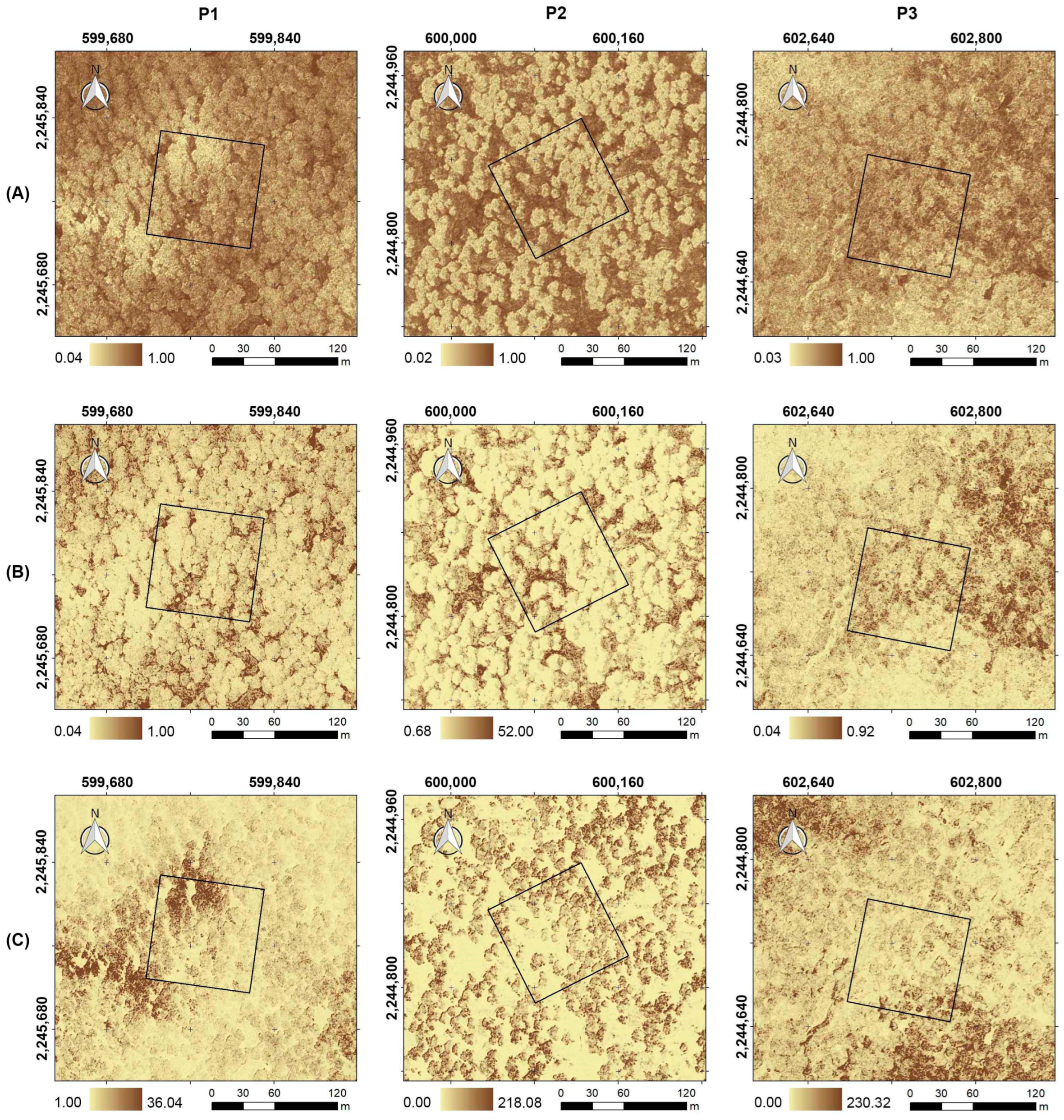
According to the VSURF algorithm, two vegetation indices and three texture bands were identified as potential explanatory variables to estimate the spatial distribution of the litter fuel loads (Figure A1 and Figure A2). Three vegetation indices and three texture bands were identified for the duff fuel loads (Figure A3 and Figure A4).
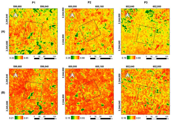
Figure A1.
Vegetation indices used to estimate the spatial distribution of litter fuel loads. P1, P2, and P3 are 1 ha sampling plots; the black solid lines represent the boundaries of each sampling plot. (A) GNDVI; (B) NDVI.
Figure A1.
Vegetation indices used to estimate the spatial distribution of litter fuel loads. P1, P2, and P3 are 1 ha sampling plots; the black solid lines represent the boundaries of each sampling plot. (A) GNDVI; (B) NDVI.
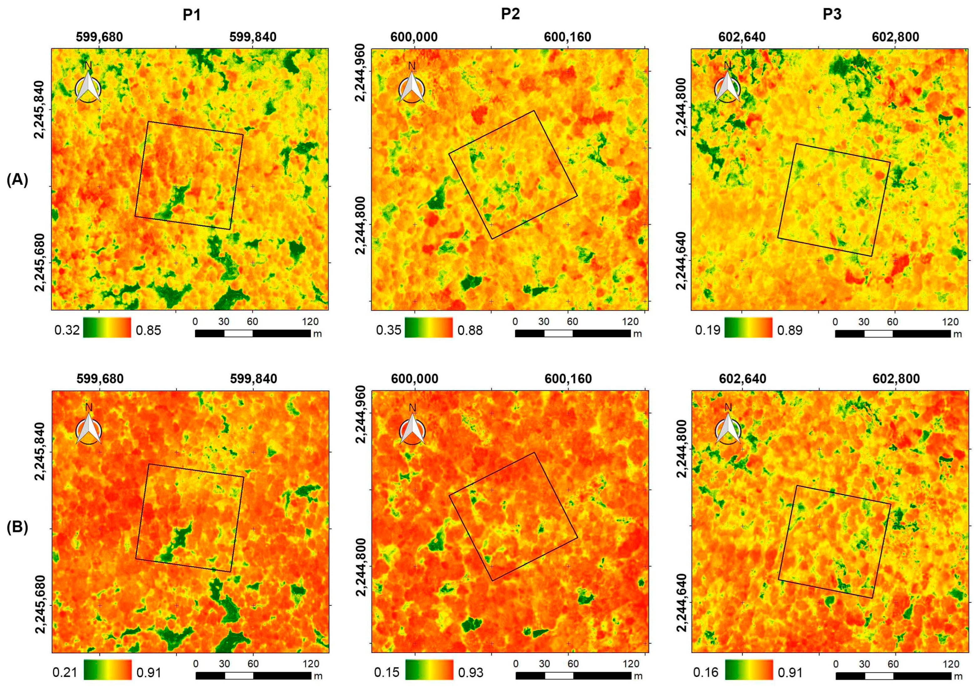
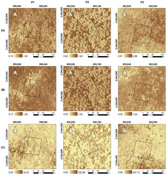
Figure A2.
Texture bands used to estimate the spatial distribution of litter fuel loads. P1, P2, and P3 are 1 ha sampling plots; the black solid lines represent the boundaries of each sampling plot. (A) Green band homogeneity texture; (B) Red band homogeneity texture; (C) Green band variance texture.
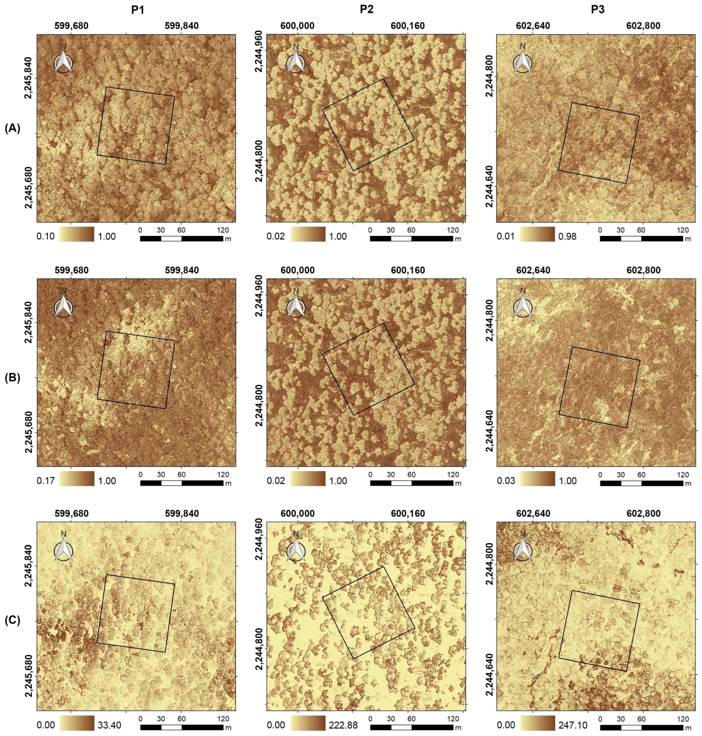

Figure A3.
Vegetation indices used to estimate the spatial distribution of duff fuel loads. P1, P2, and P3 are 1 ha sampling plots; the black solid lines represent the boundaries of each sampling plot. (A) GRVI; (B) Datt4; (C) NDVIre.
Figure A3.
Vegetation indices used to estimate the spatial distribution of duff fuel loads. P1, P2, and P3 are 1 ha sampling plots; the black solid lines represent the boundaries of each sampling plot. (A) GRVI; (B) Datt4; (C) NDVIre.
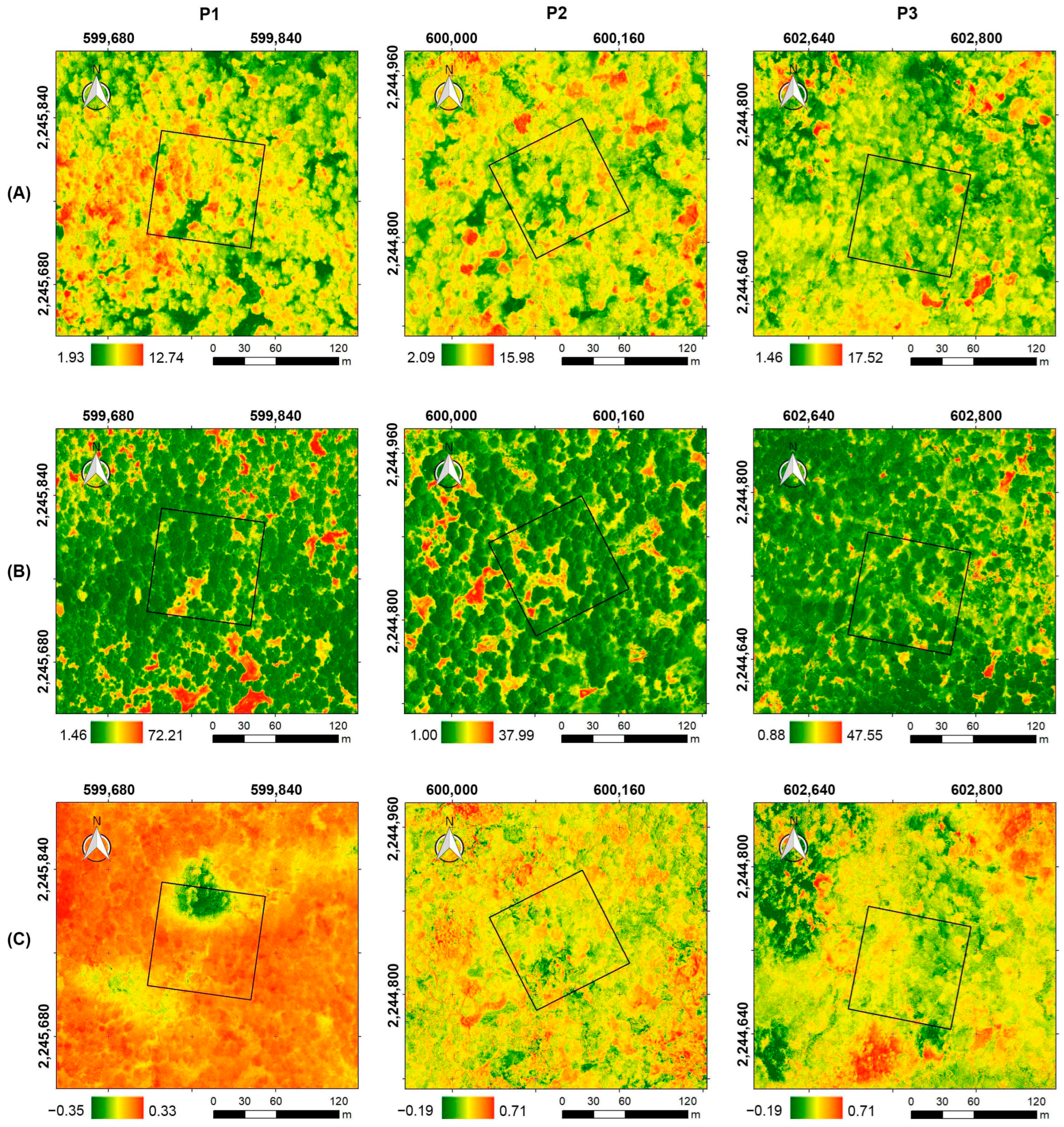
Figure A4.
Texture bands used to estimate the spatial distribution of duff fuel loads. P1, P2, and P3 are 1 ha sampling plots; the black solid lines represent the boundaries of each sampling plot. (A) Red edge band homogeneity texture; (B) Green band second moment texture; (C) Red edge band contrast texture.
References
- De Rigo, D.; Libertà, G.; Durrant, T.; Artes Vivancos, T.; San-Miguel-Ayanz, J. Forest Fire Danger Extremes in Europe Under Climate Change: Variability and Uncertainty. Ph.D. Thesis, Publications Office of the European Union, Luxembourg, 2017. [Google Scholar] [CrossRef]
- Servicio Meteorológico Nacional (SMN). Perspectiva Meteorológica Para Incendios Forestales. Available online: https://smn.conagua.gob.mx/es/incendios-forestales-diario (accessed on 11 April 2024).
- Zubkova, M.; Boschetti, L.; Abatzoglou, J.T.; Giglio, L. Changes in Fire Activity in Africa from 2002 to 2016 and Their Potential Drivers. Geophys. Res. Lett. 2019, 46, 7643–7653. [Google Scholar] [CrossRef] [PubMed]
- Pechony, O.; Shindell, D.T. Driving Forces of Global Wildfires over the Past Millennium and the Forthcoming Century. Proc. Natl. Acad. Sci. USA 2010, 107, 19167–19170. [Google Scholar] [CrossRef] [PubMed]
- Intergovernmental Panel on Climate Change (IPCC). Global Climate. Available online: https://www.ipcc.ch/report/ar4/wg1/global-climate-projections/ (accessed on 25 January 2024).
- United Nations Environment Programme (UNEP). Spreading Like Wildfire: The Rising Threat of Extraordinary Landscape Fires; United Nations Environment Programme (UNEP): Nairobi, Kenia, 2022; Available online: https://www.unep.org/resources/report/spreading-wildfire-rising-threat-extraordinary-landscape-fires (accessed on 26 August 2024).
- Aponte, C.; de Groot, W.J.; Wotton, B.M. Forest Fires and Climate Change: Causes, Consequences and Management Options. Int. J. Wildland Fire 2016, 25, 1–2. [Google Scholar] [CrossRef]
- Chuvieco, E. (Ed.) Earth Observation of Wildland Fires in Mediterranean Ecosystems; Springer: Berlin/Heidelberg, Germany, 2009. [Google Scholar] [CrossRef]
- Fried, J.S.; Gilless, J.K.; Riley, W.J.; Moody, T.J.; Simon de Blas, C.; Hayhoe, K.; Moritz, M.; Stephens, S.; Torn, M. Predicting the Effect of Climate Change on Wildfire Behavior and Initial Attack Success. Clim. Chang. 2008, 87, 251–264. [Google Scholar] [CrossRef]
- Kreider, M.R.; Higuera, P.E.; Parks, S.A.; Rice, W.L.; White, N.; Larson, A.J. Fire Suppression Makes Wildfires More Severe and Accentuates Impacts of Climate Change and Fuel Accumulation. Nat. Commun. 2024, 15, 2412. [Google Scholar] [CrossRef]
- Moghaddas, J.J.; Collins, B.M.; Menning, K.; Moghaddas, E.E.Y.; Stephens, S.L. Fuel Treatment Effects on Modeled Landscape-Level Fire Behavior in the Northern Sierra Nevada. Can. J. For. Res. 2010, 40, 1751–1765. [Google Scholar] [CrossRef]
- Tymstra, C.; Bryce, R.W.; Wotton, B.M.; Taylor, S.W.; Armitage, O.B. Development and Structure of Prometheus: The Canadian Wildland Fire Growth Simulation Model; Natural Resources Canada: Edmonton, AB, Canada, 2010. [Google Scholar]
- Furlaud, J.M.; Williamson, G.J.; Bowman, D.M.J.S. Simulating the Effectiveness of Prescribed Burning at Altering Wildfire Behaviour in Tasmania, Australia. Int. J. Wildland Fire 2018, 27, 15. [Google Scholar] [CrossRef]
- Secretaría de Medio Ambiente y Recursos Naturales (SEMARNAT). Programa de Manejo del Fuego 2020–2024; SEMARNAT: Mexico City, México, 2020. [Google Scholar]
- Keane, R.E. Wildland Fuel Fundamentals and Applications; Springer International: New York, NY, USA, 2015. [Google Scholar]
- Keane, R.E. Describing Wildland Surface Fuel Loading for Fire Management: A Review of Approaches, Methods and Systems. Int. J. Wildland Fire 2013, 22, 51. [Google Scholar] [CrossRef]
- Weise, D.R.; Cobian-Iñiguez, J.; Princevac, M. Surface to Crown Transition. In Encyclopedia of Wildfires and Wildland-Urban Interface (WUI) Fires; Springer International Publishing: Cham, Switzerland, 2018; pp. 1–5. [Google Scholar] [CrossRef]
- Scott, J.H.; Reinhardt, E.D. Assessing Crown Fire Potential by Linking Models of Surface and Crown Fire Behavior; US Department of Agriculture, Forest Service, Rocky Mountain Research Station: Fort Collins, CO, USA, 2001. [CrossRef]
- Hirsch, K.G. Canadian Forest Fire Behavior Prediction (FBP) System: User’s Guide; Natural Resources Canada, Canadian Forest Service, Northern Forestry Centre: Vancouver, BC, Canada, 1996. [Google Scholar]
- Pérez-Suárez, M.; Arredondo-Moreno, J.T.; Huber-Sannwald, E. Early Stage of Single and Mixed Leaf-Litter Decomposition in Semiarid Forest Pine-Oak: The Role of Rainfall and Microsite. Biogeochemistry 2012, 108, 245–258. [Google Scholar] [CrossRef]
- Xelhuantzi-Carmona, J.; Flores-Garnica, J.G.; Chávez-Durán, A.A. Análisis Comparativo de Cargas de Combustibles en Ecosistemas Forestales Afectados Por Incendios. Rev. Mex. Cienc. For. 2011, 2, 37–52. [Google Scholar] [CrossRef]
- Prichard, S.J.; Andreu, A.G.; Ottmar, R.D.; Eberhardt, E. Fuel Characteristic Classification System (FCCS) Field Sampling and Fuelbed Development Guide; Pacific Northwest Research Station, USDA Forest Service: Portland, OR, USA, 2019. [CrossRef]
- Finney, M.A. Fire Research and Management Exchange System. FlamMap 6.2. Available online: https://www.frames.gov/catalog/67085 (accessed on 1 May 2024).
- Arroyo, L.A.; Pascual, C.; Manzanera, J.A. Fire Models and Methods to Map Fuel Types: The Role of Remote Sensing. For. Ecol. Manag. 2008, 256, 1239–1252. [Google Scholar] [CrossRef]
- Chávez-Durán, Á.A.; Olvera-Vargas, M.; Figueroa-Rangel, B.; García, M.; Aguado, I.; Ruiz-Corral, J.A. Mapping Homogeneous Response Areas for Forest Fuel Management Using Geospatial Data, K-Means, and Random Forest Classification. Forests 2022, 13, 1970. [Google Scholar] [CrossRef]
- Mestre, L.; Toro-Manríquez, M.; Soler, R.; Huertas-Herrera, A.; Martínez-Pastur, G.; Lencinas, M.V. The Influence of Canopy-Layer Composition on Understory Plant Diversity in Southern Temperate Forests. For. Ecosyst. 2017, 4, 6. [Google Scholar] [CrossRef]
- Casals, P.; Valor, T.; Besalú, A.; Molina-Terrén, D. Understory Fuel Load and Structure Eight to Nine Years after Prescribed Burning in Mediterranean Pine Forests. For. Ecol. Manag. 2016, 362, 156–168. [Google Scholar] [CrossRef]
- Chávez-Durán, Á.A.; Bustos-Santana, A.; Chávez-Durán, H.M.; Flores-Garnica, J.G.; Rubio-Camacho, E.A.; Xelhuantzi-Carmona, J. Distribución Espacial de Cargas de Combustibles en Una Parcela de Muestreo de Pino–Encino. Rev. Mex. Cienc. For. 2021, 12, 112–133. [Google Scholar] [CrossRef]
- Flores-Garnica, J.G.; Chávez-Durán, A.A.; Rubio-Camacho, E.A.; Villela Gaytán, S.A.; Xelhuantzi-Carmona, J.; Frías-Gómez, J.G. Evaluación de la Respuesta de Diferentes Ecosistemas Forestales a los Incendios Forestales. Informe Técnico y Financiero Segunda Etapa. Clave CONACyT: 71400; Comisión Nacional Forestal of Mexico (CONAFOR): Guadalajara, Mexico, 2008; Available online: http://www.cnf.gob.mx/IMASD (accessed on 27 June 2022).
- Chávez-Durán, Á.A.; Flores-Garnica, J.G.; Luna-Luna, M.; Centeno-Erguera, L.R.; Alarcón-Bustamante, M.P. Caracterización y Clasificación de Camas de Combustibles Prioritarias en México Para Planificar el Manejo del Fuego. Informe Técnico Fondo Sectorial CONACyT-CONAFOR. Referencia: CONAFOR-2012-C01-175523; Fundamentos Técnicos y Metodológicos: Tepatitlán de Morelos, México, 2014; Available online: http://www.cnf.gob.mx/IMASD (accessed on 16 August 2022).
- Loudermilk, E.L.; O’Brien, J.J.; Goodrick, S.L.; Linn, R.R.; Skowronski, N.S.; Hiers, J.K. Vegetation’s Influence on Fire Behavior Goes beyond Just Being Fuel. Fire Ecol. 2022, 18, 9. [Google Scholar] [CrossRef]
- Chávez-Durán, Á.A.; García, M.; Olvera-Vargas, M.; Aguado, I.; Figueroa-Rangel, B.L.; Trucíos-Caciano, R.; Rubio-Camacho, E.A. Forest Canopy Fuel Loads Mapping Using Unmanned Aerial Vehicle High-Resolution Red, Green, Blue and Multispectral Imagery. Forests 2024, 15, 225. [Google Scholar] [CrossRef]
- García, M.; Popescu, S.; Riaño, D.; Zhao, K.; Neuenschwander, A.; Agca, M.; Chuvieco, E. Characterization of Canopy Fuels Using ICESat/GLAS Data. Remote Sens. Environ. 2012, 123, 81–89. [Google Scholar] [CrossRef]
- Botequim, B.; Fernandes, P.M.; Borges, J.G.; González-Ferreiro, E.; Guerra-Hernández, J. Improving Silvicultural Practices for Mediterranean Forests through Fire Behaviour Modelling Using LiDAR-Derived Canopy Fuel Characteristics. Int. J. Wildland Fire 2019, 28, 823. [Google Scholar] [CrossRef]
- Aragoneses, E.; García, M.; Ruiz-Benito, P.; Chuvieco, E. Mapping Forest Canopy Fuel Parameters at European Scale Using Spaceborne LiDAR and Satellite Data. Remote Sens. Environ. 2024, 303, 114005. [Google Scholar] [CrossRef]
- Aragoneses, E.; García, M.; Salis, M.; Ribeiro, L.M.; Chuvieco, E. Classification and Mapping of European Fuels Using a Hierarchical, Multipurpose Fuel Classification System. Earth Syst. Sci. Data 2023, 15, 1287–1315. [Google Scholar] [CrossRef]
- Abdollahi, A.; Yebra, M. Forest Fuel Type Classification: Review of Remote Sensing Techniques, Constraints and Future Trends. J. Environ. Manag. 2023, 342, 118315. [Google Scholar] [CrossRef] [PubMed]
- Flores-Garnica, J.G. Antecedentes y Perspectivas de La Investigación En Incendios Forestales En El INIFAP. Rev. Mex. Cienc. For. 2021, 12, 91–119. [Google Scholar] [CrossRef]
- Arellano-Pérez, S.; Castedo-Dorado, F.; López-Sánchez, C.; González-Ferreiro, E.; Yang, Z.; Díaz-Varela, R.; Álvarez-González, J.; Vega, J.; Ruiz-González, A. Potential of Sentinel-2A Data to Model Surface and Canopy Fuel Characteristics in Relation to Crown Fire Hazard. Remote Sens. 2018, 10, 1645. [Google Scholar] [CrossRef]
- Franke, J.; Barradas, A.C.S.; Borges, M.A.; Menezes Costa, M.; Dias, P.A.; Hoffmann, A.A.; Orozco Filho, J.C.; Melchiori, A.E.; Siegert, F. Fuel Load Mapping in the Brazilian Cerrado in Support of Integrated Fire Management. Remote Sens. Environ. 2018, 217, 221–232. [Google Scholar] [CrossRef]
- Labenski, P.; Ewald, M.; Schmidtlein, S.; Heinsch, F.A.; Fassnacht, F.E. Quantifying Surface Fuels for Fire Modelling in Temperate Forests Using Airborne Lidar and Sentinel-2: Potential and Limitations. Remote Sens. Environ. 2023, 295, 113711. [Google Scholar] [CrossRef]
- Li, S.; Wang, T.; Hou, Z.; Gong, Y.; Feng, L.; Ge, J. Harnessing Terrestrial Laser Scanning to Predict Understory Biomass in Temperate Mixed Forests. Ecol. Indic. 2021, 121, 107011. [Google Scholar] [CrossRef]
- Maesano, M.; Santopuoli, G.; Moresi, F.; Matteucci, G.; Lasserre, B.; Scarascia Mugnozza, G. Above Ground Biomass Estimation from UAV High Resolution RGB Images and LiDAR Data in a Pine Forest in Southern Italy. IForest 2022, 15, 451–457. [Google Scholar] [CrossRef]
- Zhang, Z.; Zhu, L. A Review on Unmanned Aerial Vehicle Remote Sensing: Platforms, Sensors, Data Processing Methods, and Applications. Drones 2023, 7, 398. [Google Scholar] [CrossRef]
- Hoffrén, R.; Lamelas, M.T.; de la Riva, J. UAV-Derived Photogrammetric Point Clouds and Multispectral Indices for Fuel Estimation in Mediterranean Forests. Remote Sens. Appl. 2023, 31, 100997. [Google Scholar] [CrossRef]
- Comisión Nacional de Áreas Naturales Protegidas (CONANP). Recategorización del Área de Protección de Flora y Fauna “Sierra de Quila”; Diario Oficial: Mexico City, Mexico, 2000; pp. 1–5. Available online: https://simec.conanp.gob.mx/pdf_recategorizacion/64_reca.pdf (accessed on 27 June 2022).
- Jardel-Pelaez, E.J.; Pérez-Salicrup, D.; Alvarado-Celestino, E.; Morfin-Rios, J.E. Principios y Criterios Para el Manejo del Fuego en Ecosistemas Forestales: Guía de Campo; Comisión Nacional Forestal: Guadalajara, México, 2014. [Google Scholar]
- Jiménez-Luquín, E. Sierra de Quila: ¿Cómo Ha Ido Cambiando Los Últimos 25 Años Desde La Tragedia? In Memorias. I Foro de Conocimiento, Uso y Gestión del Área Natural Protegida Sierra de Quila; Villavicencio-García, R., Santiago-Pérez, A.L., Rosas-Espinoza, V.C., Hernández-López, L., Eds.; Universidad de Guadalajara, Centro Universitario de Ciencias Biológicas y Agropecuarias, Departamento de Producción Forestal: Guadalajara, México, 2011; pp. 1–134. [Google Scholar]
- Fox, J.; Weisberg, S. An R Companion to Applied Regression, 3rd ed.; Sage: California, CA, USA, 2018. [Google Scholar]
- Vargha, A.; Delaney, H.D. The Kruskal-Wallis Test and Stochastic Homogeneity. J. Educ. Behav. Stat. 1998, 23, 170–192. [Google Scholar] [CrossRef]
- Bonamente, M. Statistics and Analysis of Scientific Data; Springer Science and Business Media: New York, NY, USA, 2017. [Google Scholar]
- Keane, R.E.; Gray, K.; Bacciu, V.; Leirfallom, S. Spatial Scaling of Wildland Fuels for Six Forest and Rangeland Ecosystems of the Northern Rocky Mountains, USA. Landsc. Ecol. 2012, 27, 1213–1234. [Google Scholar] [CrossRef]
- Siabato, W.; Guzmán-Manrique, J. La Autocorrelación Espacial y El Desarrollo de La Geografía Cuantitativa. Cuad. Geogr. Rev. Colomb. Geogr. 2019, 28, 1–22. [Google Scholar] [CrossRef]
- Poncet, A.M.; Knappenberger, T.; Brodbeck, C.; Fogle, M.; Shaw, J.N.; Ortiz, B.V. Multispectral UAS Data Accuracy for Different Radiometric Calibration Methods. Remote Sens. 2019, 11, 1917. [Google Scholar] [CrossRef]
- Park, J.W.; Yeom, D.J. Method for Establishing Ground Control Points to Realize UAV-Based Precision Digital Maps of Earthwork Sites. J. Asian Archit. Build. Eng. 2022, 21, 110–119. [Google Scholar] [CrossRef]
- Westoby, M.J.; Brasington, J.; Glasser, N.F.; Hambrey, M.J.; Reynolds, J.M. ‘Structure-from-Motion’ Photogrammetry: A Low-Cost, Effective Tool for Geoscience Applications. Geomorphology 2012, 179, 300–314. [Google Scholar] [CrossRef]
- Agisoft LLC. Agisoft Metashape User Manual; Agisoft LLC: St. Petersburg, Russia, 2023. [Google Scholar]
- Barrett, F.; McRoberts, R.E.; Tomppo, E.; Cienciala, E.; Waser, L.T. A Questionnaire-Based Review of the Operational Use of Remotely Sensed Data by National Forest Inventories. Remote Sens. Environ. 2016, 174, 279–289. [Google Scholar] [CrossRef]
- Guerini-Filho, M.; Kuplich, T.M.; De Quadros, F.L.F. Estimating Natural Grassland Biomass by Vegetation Indices Using Sentinel 2 Remote Sensing Data. Int. J. Remote Sens. 2020, 41, 2861–2876. [Google Scholar] [CrossRef]
- Warner, T. Kernel-Based Texture in Remote Sensing Image Classification. Geogr. Compass 2011, 5, 781–798. [Google Scholar] [CrossRef]
- Kupidura, P. The Comparison of Different Methods of Texture Analysis for Their Efficacy for Land Use Classification in Satellite Imagery. Remote Sens. 2019, 11, 1233. [Google Scholar] [CrossRef]
- Haralick, R.M.; Shanmugam, K.; Dinstein, I. Textural Features for Image Classification. IEEE Trans. Syst. Man Cybern. 1973, SMC-3, 610–621. [Google Scholar] [CrossRef]
- Pal, M. Random Forest Classifier for Remote Sensing Classification. Int. J. Remote Sens. 2005, 26, 217–222. [Google Scholar] [CrossRef]
- Ganesh, N.; Jain, P.; Choudhury, A.; Dutta, P.; Kalita, K.; Barsocchi, P. Random Forest Regression-Based Machine Learning Model for Accurate Estimation of Fluid Flow in Curved Pipes. Processes 2021, 9, 2095. [Google Scholar] [CrossRef]
- Genuer, R.; Poggi, J.-M.; Tuleau-Malot, C. VSURF: An R Package for Variable Selection Using Random Forests. R J. 2015, 7, 19. [Google Scholar] [CrossRef]
- Han, H.; Guo, X.; Yu, H. Variable Selection Using Mean Decrease Accuracy and Mean Decrease Gini Based on Random Forest. In Proceedings of the 2016 7th IEEE International Conference on Software Engineering and Service Science (ICSESS), Beijing, China, 26–28 August 2016; IEEE: New York, NY, USA, 2016; pp. 219–224. [Google Scholar] [CrossRef]
- Liaw, A.; Wiener, M.; Breiman, L.; Cutler, A. Package ‘randomForest’. Breiman and Cutler’s Random Forests for Classification and Regression. Available online: https://cran.r-project.org/web/packages/randomForest/randomForest.pdf (accessed on 18 March 2024).
- Hijmans, R.J. Package ‘Raster’. Geographic Data Analysis and Modeling. Available online: https://cran.r-project.org/web/packages/raster/raster.pdf (accessed on 18 March 2024).
- Pebesma, E. Package ‘sf’. Simple Features for R. Available online: https://cran.r-project.org/web/packages/sf/sf.pdf (accessed on 19 March 2024).
- R Core Team. R: A Language and Environment for Statistical Computing. Available online: https://www.R-project.org/ (accessed on 15 June 2024).
- McRoberts, R.E.; Magnussen, S.; Tomppo, E.O.; Chirici, G. Parametric, Bootstrap, and Jackknife Variance Estimators for the k-Nearest Neighbors Technique with Illustrations Using Forest Inventory and Satellite Image Data. Remote Sens. Environ. 2011, 115, 3165–3174. [Google Scholar] [CrossRef]
- García, M.; Saatchi, S.; Casas, A.; Koltunov, A.; Ustin, S.; Ramirez, C.; Balzter, H. Extrapolating Forest Canopy Fuel Properties in the California Rim Fire by Combining Airborne LiDAR and Landsat OLI Data. Remote Sens. 2017, 9, 394. [Google Scholar] [CrossRef]
- Breiman, L. Random Forests. Mach. Learn. 2001, 45, 5–32. [Google Scholar] [CrossRef]
- Brede, B.; Terryn, L.; Barbier, N.; Bartholomeus, H.M.; Bartolo, R.; Calders, K.; Derroire, G.; Krishna Moorthy, S.M.; Lau, A.; Levick, S.R.; et al. Non-Destructive Estimation of Individual Tree Biomass: Allometric Models, Terrestrial and UAV Laser Scanning. Remote Sens. Environ. 2022, 280, 113180. [Google Scholar] [CrossRef]
- Wickham, H.; Hester, J.; Francois, R.; Bryan, J.; Bearrows, S.; Jylänki, J.; Jørgensen, M. Package ‘Readr.’ Read Rectangular Text Data. Available online: https://cran.r-project.org/web/packages/readr/readr.pdf (accessed on 15 June 2024).
- Gross, J.; Ligges, U. Package ‘Northest.’ Tests for Normality. Available online: https://cran.r-project.org/web/packages/nortest/nortest.pdf (accessed on 15 June 2023).
- Fox, J.; Weisberg, S.; Price, B.; Adler, D.; Bates, D.; Baud-Bovy, G.; Bolker, B.; Ellison, S.; Firth, D.; Friendly, M.; et al. Package ‘Car’. Companion to Applied Regression. Available online: https://cran.r-project.org/web/packages/car/car.pdf (accessed on 7 July 2023).
- Husson, F.; Josse, J.; Le, S.; Mazet, J. Package ‘FactoMineR’. Available online: https://cran.r-project.org/web/packages/FactoMineR/FactoMineR.pdf (accessed on 16 September 2023).
- Wright, M.; Wager, S.; Probst, P. Package ‘Ranger’. A Fast Implementation of Random Forests. Available online: https://cran.r-project.org/web/packages/ranger/ranger.pdf (accessed on 3 June 2024).
- Wickham, H.; Chang, W.; Henry, L.; Lin-Pedersen, T.; Takahashi, K.; Wilke, C.; Woo, K.; Yutani, H.; Dunnington, D. Package ‘ggplot2.’ Create Elegant Data Visualisations Using the Grammar of Graphics. Available online: https://cran.r-project.org/web/packages/ggplot2/ggplot2.pdf (accessed on 7 July 2023).
- Ulrich, W.; Piwczyński, M.; Zaplata, M.K.; Winter, S.; Schaaf, W.; Fischer, A. Small-Scale Spatial Variability in Phylogenetic Community Structure during Early Plant Succession Depends on Soil Properties. Oecologia 2014, 175, 985–995. [Google Scholar] [CrossRef]
- Doro, L.; Meinardus, A.; Jeong, J.; Osorio-Leyton, J.M.; Steglich, E.M. Environmental Policy Integrated Climate (EPIC) User Manual; Texas A&M: Temple, TX, USA, 2024. [Google Scholar]
- Kwon, T.; Shibata, H.; Kepfer-Rojas, S.; Schmidt, I.K.; Larsen, K.S.; Beier, C.; Berg, B.; Verheyen, K.; Lamarque, J.-F.; Hagedorn, F.; et al. Effects of Climate and Atmospheric Nitrogen Deposition on Early to Mid-Term Stage Litter Decomposition Across Biomes. Front. For. Glob. Chang. 2021, 4, 678480. [Google Scholar] [CrossRef]
- Austin, A.T.; Vitousek, P.M. Precipitation, Decomposition and Litter Decomposability of Metrosideros Polymorpha in Native Forests on Hawai’i. J. Ecol. 2000, 88, 129–138. [Google Scholar] [CrossRef]
- Mohammadpour, P.; Viegas, D.X.; Viegas, C. Vegetation Mapping with Random Forest Using Sentinel 2 and GLCM Texture Feature—A Case Study for Lousã Region, Portugal. Remote Sens. 2022, 14, 4585. [Google Scholar] [CrossRef]
- Ishihara, M.I.; Hiura, T. Modeling Leaf Area Index from Litter Collection and Tree Data in a Deciduous Broadleaf Forest. Agric. For. Meteorol. 2011, 151, 1016–1022. [Google Scholar] [CrossRef]
- Raaflaub, L.D.; Valeo, C. Assessing Factors That Influence Spatial Variations in Duff Moisture. Hydrol. Process. 2008, 22, 2874–2883. [Google Scholar] [CrossRef]
- Rubio-Camacho, E.A. Análisis de La Estructura, Biomasa y Combustibles Forestales: Una Aproximación a la Ecología del Fuego en Bosques Montanos de la Sierra Madre Oriental, Universidad Autónoma de Nuevo León, Linares, Nuevo León, Mexico. 2013. Available online: http://eprints.uanl.mx/5714/ (accessed on 28 June 2022).
- del Río, M.; Löf, M.; Bravo-Oviedo, A.; Jactel, H. Understanding the Complexity of Mixed Forest Functioning and Management: Advances and Perspectives. For. Ecol. Manag. 2021, 489, 119138. [Google Scholar] [CrossRef]
- Bergamo, T.F.; de Lima, R.S.; Kull, T.; Ward, R.D.; Sepp, K.; Villoslada, M. From UAV to PlanetScope: Upscaling Fractional Cover of an Invasive Species Rosa Rugosa. J. Environ. Manag. 2023, 336, 117693. [Google Scholar] [CrossRef]
Disclaimer/Publisher’s Note: The statements, opinions and data contained in all publications are solely those of the individual author(s) and contributor(s) and not of MDPI and/or the editor(s). MDPI and/or the editor(s) disclaim responsibility for any injury to people or property resulting from any ideas, methods, instructions or products referred to in the content. |
© 2024 by the authors. Licensee MDPI, Basel, Switzerland. This article is an open access article distributed under the terms and conditions of the Creative Commons Attribution (CC BY) license (https://creativecommons.org/licenses/by/4.0/).

