Comparing Accuracy of Wildfire Spread Prediction Models under Different Data Deficiency Conditions

Abstract

Wildfire is one of the most severe natural disasters globally, profoundly affecting natural ecology, economy, and health and safety. Precisely predicting the spread of wildfires has become an important research topic. Current fire spread prediction models depend on inputs from a variety of geographical and environmental variables. However, unlike the ideal conditions simulated in the laboratory, data gaps often occur in real wildfire scenarios, posing challenges to the accuracy and robustness of predictions. It is necessary to explore the extent to which different missing items affect prediction accuracy, thereby providing rational suggestions for emergency decision-making. In this paper, we tested how different conditions of missing data affect the prediction accuracy of existing wildfire spread models and quantified the corresponding errors. The final experimental results suggest that it is necessary to judge the potential impact of data gaps based on the geographical conditions of the study area appropriately, as there is no significant pattern of behavior yet identified. This study aims to simulate the impact of data scarcity on the accuracy of wildfire spread prediction models in real scenarios, thereby enabling researchers to better understand the priority of different environmental variables for the model and identify the acceptable degree of missing data and the indispensable data attributes. It offers new insights for developing spread prediction models applicable to real-world scenarios and rational assessment of the effectiveness of model outcomes.

1. Introduction

Wildfires, being among the most severe natural calamities, significantly affect ecosystems, economic conditions, and human well-being and security [1]. In just one instance in July 2023, there were 5082 wildfire cases in Canada, burning over 1.3 million hectares of land, which is about 4% of Canada’s entire forest area [2]. Rapid and proper wildfire management is closely related to the ability to accurately predict wildfire spread. In the past, several wildfire spread prediction models such as the classic FARSITE [3], BehavePlus [4], WRF-SFIRE [5], the more recent CA Model [6], and WFNet [7] have been developed and widely applied to actual wildfire events. However, numerous studies [8,9] have shown that such modeling approaches are highly sensitive to environmental parameters (e.g., the allocation of fuel models and changes in the locations of ignition points), resulting in significant predictive uncertainties. What is worse, under real wildfire scenarios, some environmental data may suffer from quality deterioration or even become entirely missing. Such situations have been also confirmed in actual emergency decision-making processes, where the urgency of time leads to issues like time-related decay and incomplete data, making it difficult to judge the validity of the model’s predictive outcomes. These circumstances present new challenges for wildfire spread modelling.

Modeling complex environmental phenomena is filled with uncertainty [10], and wildfire behavior is no exception. This ongoing uncertainty still stems from the input data set, especially regarding wind speed, wind direction, fuel model allocation, and the location and timing of ignitions. Thompson et al. [11] summarized the sources of various uncertainties in wildfires, while Yuan et al. [12] explained the causes of model uncertainties from a physical mechanism standpoint. In the past, numerous scholars have systematically studied the sensitivity of such parameters. Cai et al. [13] conducted a study in the forests of Northeast China to investigate the impact of fuel model distribution on prediction accuracy, and DeCastro et al. [14] applied the Monte Carlo method to examine the effect of ignition point location on prediction accuracy. Valero et al. [15] proposed a multifidelity method to quantitatively analyze the sensitivity of predicted fire spread velocity to weather and fuel parameters. Additionally, some scholars have examined the impact of data resolution quality on model accuracy. Ciri et al. [16] started with the spatial resolution of weather data to explore the error it caused in the simulation of atmosphere-coupled wildfire spread.

However, it is not just a simple matter of parameter changes; in real-world wildfire scenarios, it is often difficult to collect specific environmental data, leading to the worst-1 situation—complete absence of data attributes. This poses a tremendous challenge for the accuracy of wildfire spread prediction models. To date, no scholar has studied such extreme cases of data absence, but we believe it will prompt a reevaluation of the universality of wildfire spread prediction models. It is necessary to quantify the errors caused by the lack of data attributes on the accuracy of the model. We need to comprehensively explore the impact of missing geographic and environmental data under different conditions on prediction accuracy and attempt to reveal the relative importance of different input parameters, so as to avoid the risk of data omission and scientifically assist in emergency decision-making. It will also encourage the search for methods to resolve such real-world contradictions and inspire new approaches to develop spread modeling methods applicable to actual scenarios.

In this paper, we use the FARSITE model as a benchmark, simulating the absence of environmental variables by inputting pseudo-data, to study the impact of missing different data attributes on model prediction accuracy, and finally, we visualize the inferred fire perimeters, quantifying the error of the output results. We conducted experiments based on two highly representative real fire cases, analyzed the reasons for the decline in accuracy, and summarized certain patterns from them. Furthermore, we discussed the differences among existing evaluation metrics to encourage the development of more general methods.

The main contributions of our work are as follows:

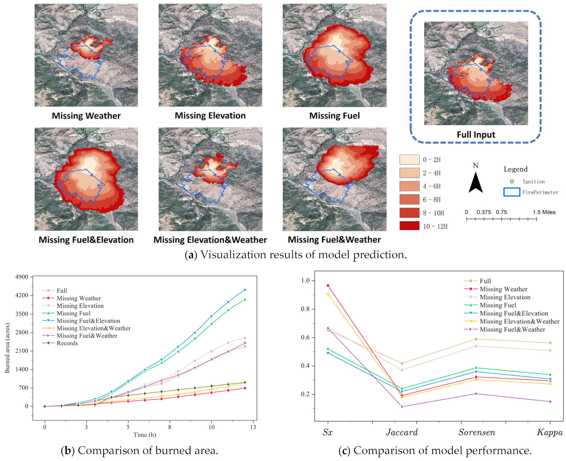
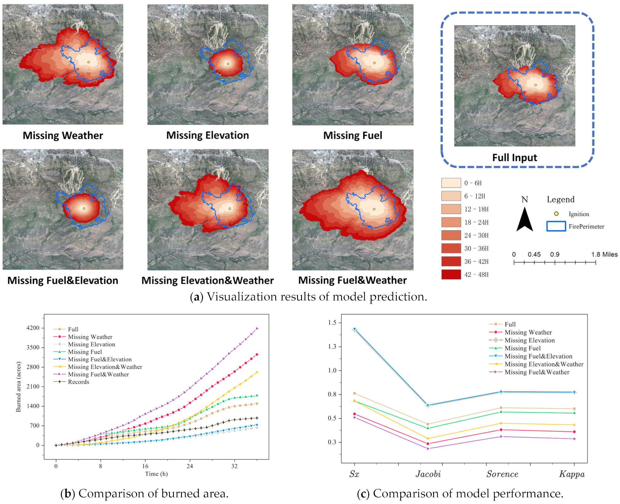
• We assessed the impact of missing data (e.g., topographic, fuel, and weather items) on the accuracy of wildfire spread models, visualized the final results, and quantified the prediction errors;
• Based on the assessment results, we analyzed the potential causes of the decline in accuracy and evaluation metrics, providing new insights for the development of universally applicable prediction models in the future.

2. Materials and Methods

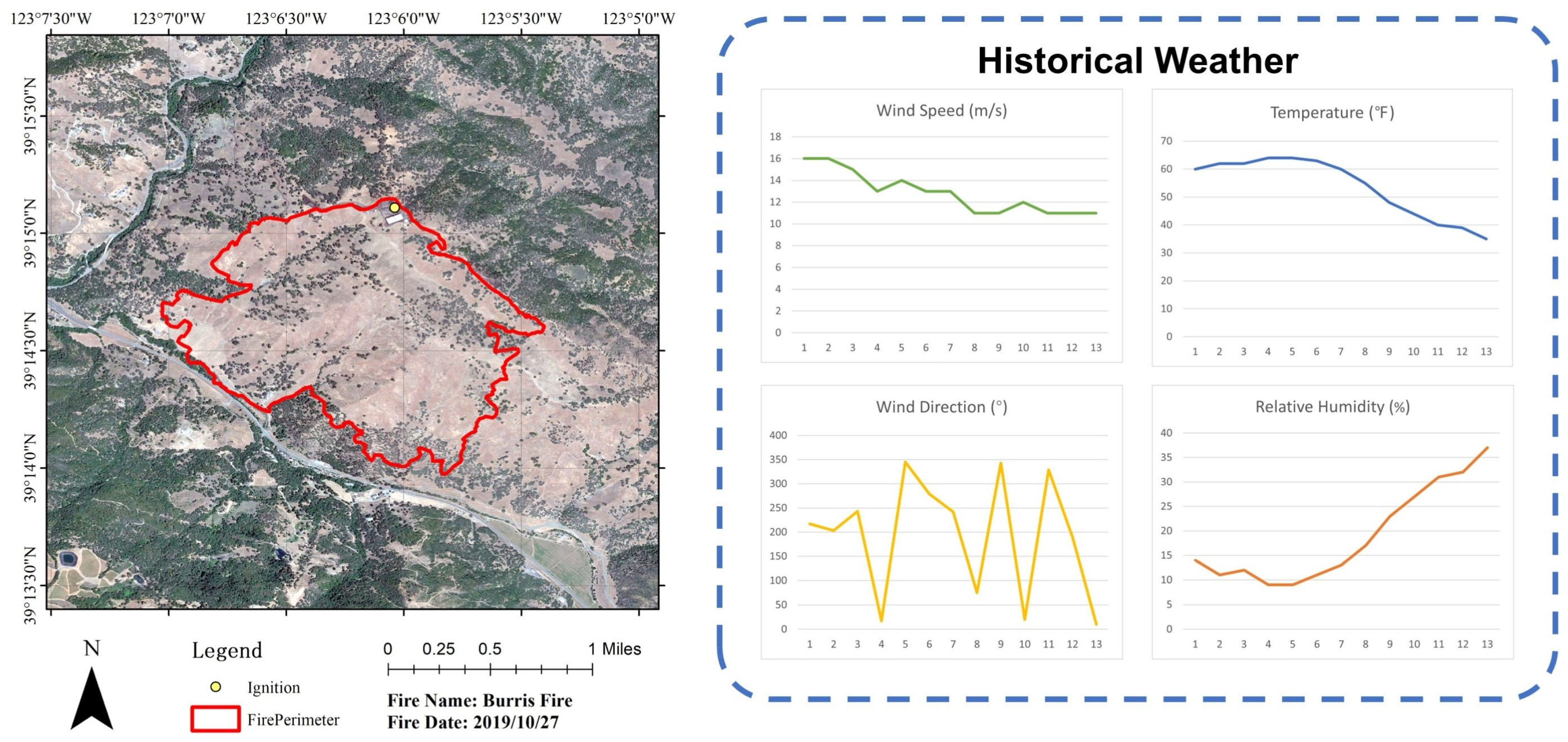
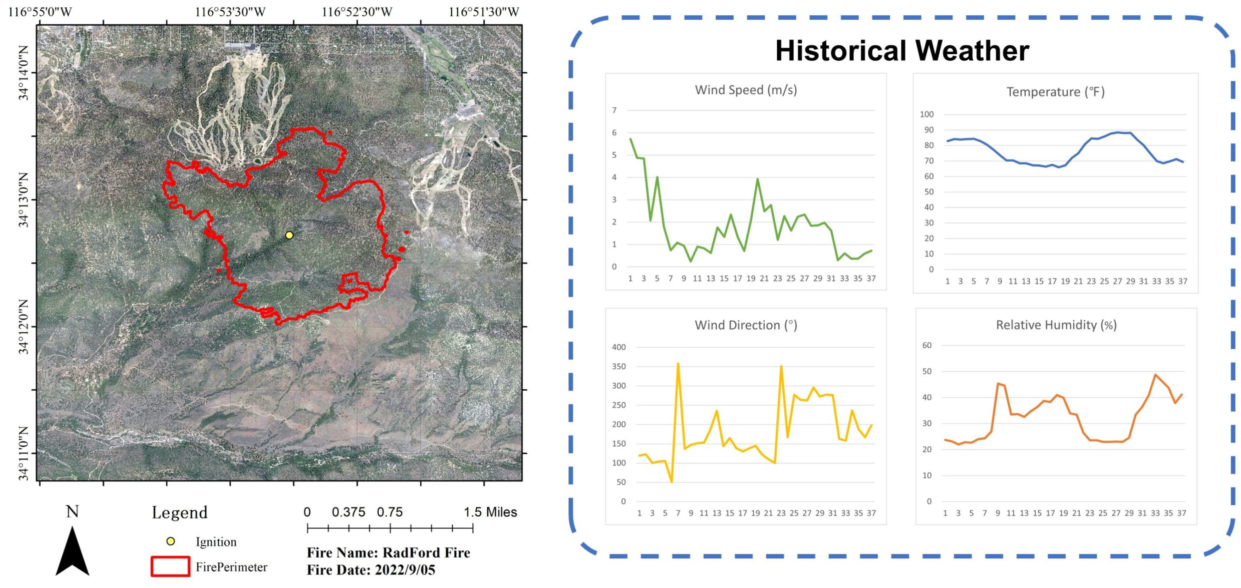
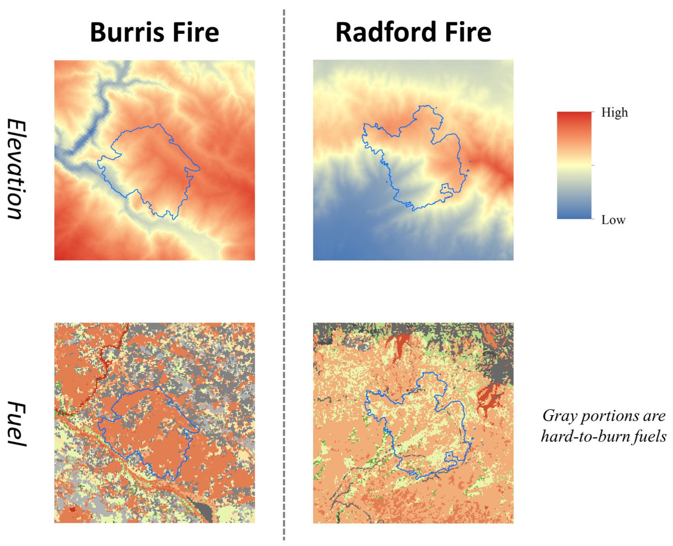
2.1. Experimental Area

We selected two real wildfire cases as experimental areas, with the basic information shown in

Table 1. Basic information of Burris Fire and Radford Fire.

Name	Date	Duration (h)	Location	Burned Area (Acre)	Fuel
Burris Fire	28 October 2019 01:34	10	34.096° N 118.481° W	704	Grass
Radford Fire	5 September 2022 12:00	50	34.177° N 116.882° W	1100	Forest

. One of the fires is named the Burris Fire, which occurred on 28 October 2019, at 01:34, spreading for nearly 10 h until it was almost completely controlled by firefighters. The ignition location was at 34.096° N, 118.481° W, and the final burned area was approximately 704 acres, involving a grassland fire. The other fire is named the Radford Fire, which occurred on 5 September 2022, at 12:00, spreading for nearly 50 h until it was eventually controlled. Its ignition point was at 34.177° N, 116.882° W, resulting in around 1100 acres of burned area, primarily involving trees, shrubs, and grass.

These two regions have highly representative geographical characteristics, with significant variations in one certain geographical variable. This can satisfy our exploration of the impact of different data attributes on the simulation results. We will analyze this point in detail in the subsequent discussion sections.

We collected the fire perimeter data, geographical data, and weather data from GeoMAC [17], LANDFIRE [18], and MesoWest [19], respectively. Additionally, the timelines of the two wildfire events are gathered from news reports [20,21,22], with specific case information illustrated in Figure 1 and Figure 2.

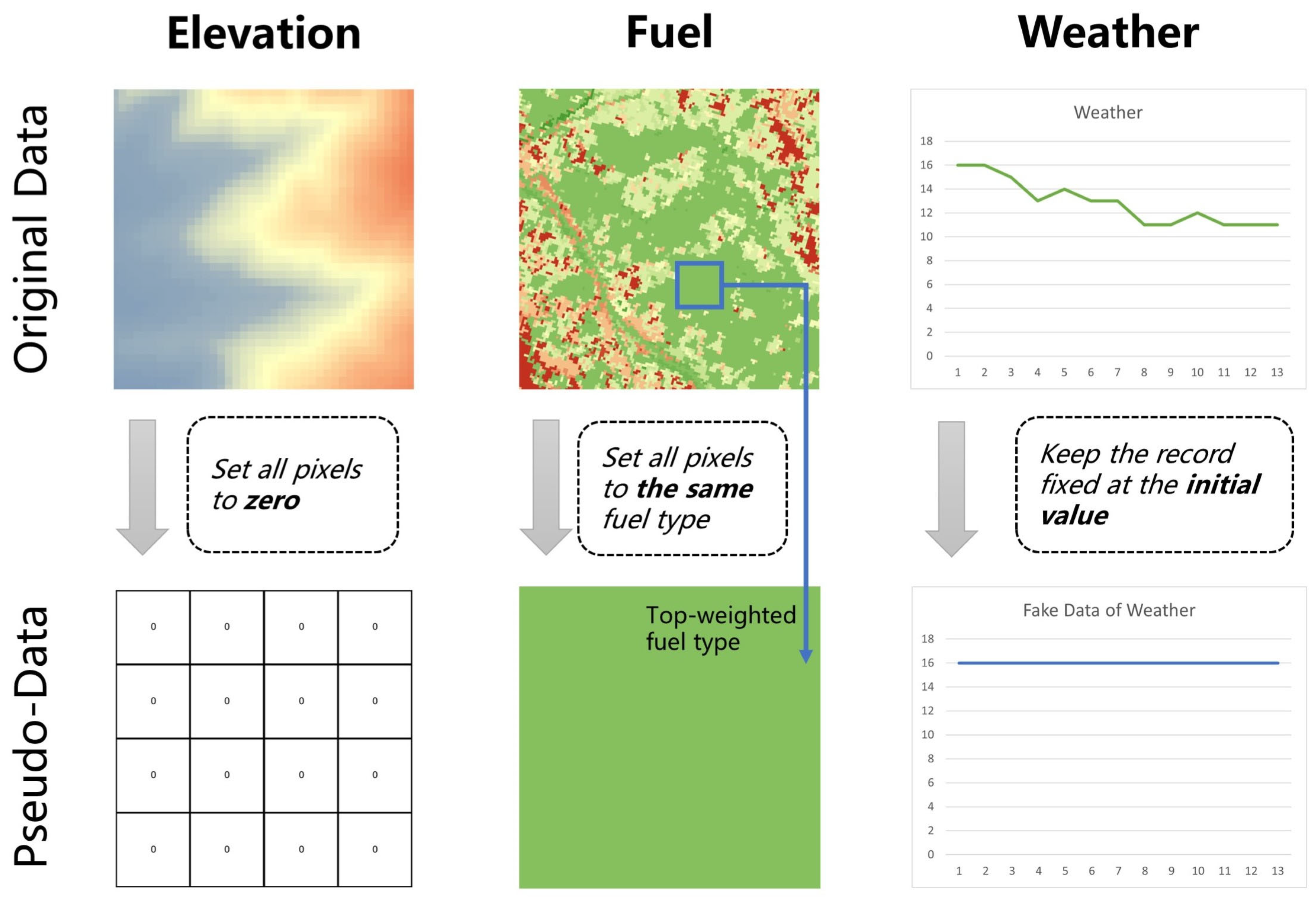
2.2. Pseudo-Data Generation

FARSITE (Fire Area Simulator) is a fire growth simulation modeling system developed by the U.S. Forest Service [3]. It is designed to simulate the spread and behavior of wildland fires under various conditions, such as fuel types, weather, and topography. The model has been widely used in fire management, planning, and research since its introduction in the mid-1990s [23].

The core principles of FARSITE involve integrating spatial data, mathematical models, and user-defined parameters to simulate fire growth over time. The main components and computational formulas used in FARSITE are the Rothermel surface fire spread model [24]; The Rothermel model calculates the rate of fire spread (R) based on the following equation:

$$\mathrm{R}=\mathrm{IR}\times \xi \times (1+{\Phi }_{\mathrm{w}}+{\Phi }_{\mathrm{s}})$$

(1)

where IR is the reaction intensity, $\xi$ is the propagating flux ratio, ${\Phi }_{\mathrm{w}}$ and ${\Phi }_{\mathrm{s}}$ are the wind and slope factors, respectively.

To produce accurate simulation results using FARSITE engine, it requires input data regarding fuel models (including fuel distribution and fuel moisture), weather data (including humidity, temperature, wind, and precipitation), as well as elevation data (including aspect, slope and elevation), and finally, an ignition point to begin operation. We will analyze how these variables influence the model’s operation from the perspective of the formulas.

Elevation data (elevation, slope, and aspect): Influence fire spread, rate of spread, and solar radiation received by the fuel bed. Slope is used in the Rothermel surface fire spread model to calculate the slope factor (${\Phi }_{\mathrm{s}}$) using the following equation: ${\Phi }_{\mathrm{s}}=5.275 \times {\beta }^{-0.3}\times {\tan \theta }^2$, where β is the packing ratio of the fuel bed and θ is the slope angle.

Fuel model (fuel model, canopy cover, and crown base height): Determines surface fuel properties, critical surface fire intensity for crown fire initiation, and crown fire behavior. The Van Wagner crown fire initiation model uses canopy cover and crown base height (CBH) to calculate the critical surface fire intensity (${\mathrm{I}}_{\mathrm{o}}$) required for crown combustion: ${\mathrm{I}}_{\mathrm{o}}={(0.01\times \mathrm{CBH}\times (460+25.9\times \mathrm{FMC}\left)\right)}^{1.5}$, where FMC is the foliar moisture content.

Weather data (wind speed and direction, temperature, relative humidity, and precipitation): Affect fuel moisture content, fire behavior, and rate of spread through the wind factor and reaction intensity. The Rothermel model incorporates wind effects through the wind factor (${\Phi }_{\mathrm{w}}$), which is calculated using the wind speed and the surface area-to-volume ratio of the fuel bed. Temperature and relative humidity influence the reaction intensity (IR) in the Rothermel model.

In real emergency management scenarios, particularly under some extreme conditions, it is often impossible to quickly and timely obtain local fuel, weather, and elevation information. These data cannot always be collected promptly from the disaster site, and in these instances, we still need to make preliminary judgments using the existing data.

In order to better explore the possible impacts of these data attributes, we need to summarize a well-established pattern of deficiency in the data, such as local inaccuracies for weather data or small-scale inaccuracies for elevation data. We then use these patterns of behavior to generate pseudo-data to derive a more quantitative level of impact. In the case of weather and elevation data, we can make the pseudo-data fluctuate over the real data, and in the case of the fuel model, we can subjectively assume that there is only a single fuel distribution within the study area to simulate the inability to survey the fuel distribution in the field. However, it is important to note that this paper simplifies this issue by considering only the extreme case of missing data, and in the future, we will propose a set of more realistic and pervasive pseudo-data generation methods to explore the impact of degraded data quality in detail.

The following methods were used to generate empty pseudo-data for the corresponding data attributes (Figure 3):

• Elevation data: Raster data with all pixels set to zero were generated according to the original data range and resolution to simulate unknown elevation conditions;
• Fuel model: Based on the most prevalent type of fuel in the burning area, raster data with all pixels set to the same fuel type were also created according to the original data range and resolution;
• Weather data: It was assumed that all weather elements remained constant from the start of the fire, and from this, pseudo-weather data were generated.

With these data generation methods, we simulate scenarios of missing data attributes. After combining different missing conditions, we conduct experiments on two fire cases.

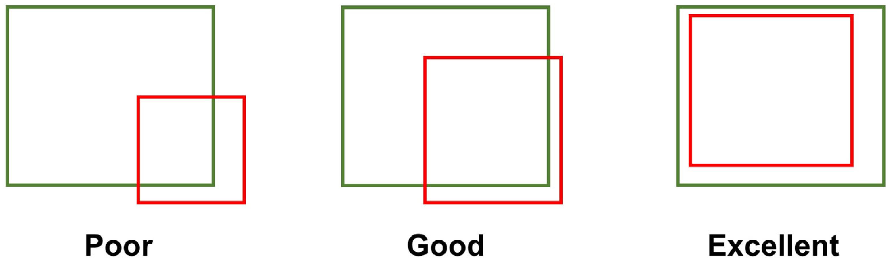
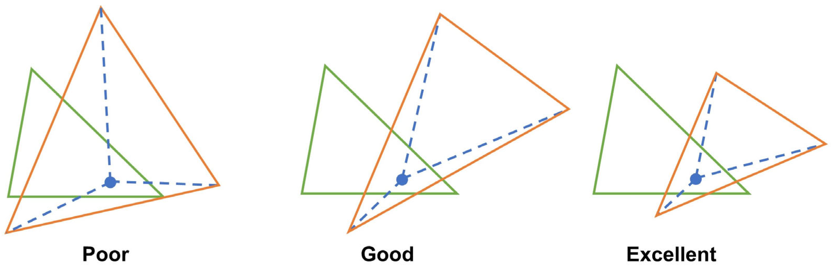
2.3. Evaluation Metrics

Many evaluation metrics for wildfire prediction models have been proposed to measure the similarity between the predictive fire perimeter and real perimeter [25]. Here, we quantitatively evaluate model performance using the Jaccard coefficient [26], Sorensen metric [27], Kappa statistics [23], and perimeter size differences Sx [28], as shown in Equations (2)–(6). Among them, higher values of the Jaccard coefficient, Sorensen metric, and Kappa statistics indicate better performance, whereas an Sx value closer to 1 is preferable.

The Jaccard coefficient specifically calculates the degree of inter agreement between two sets. Here, the two sets are the simulated and observed burned areas. The intersection of the two burned areas is divided by the total burned areas. The Sorensen metric is also a straightforward comparison method. The value is defined as the area of the intersection divided by the area of the union of the two sample sets (simulated and observed burned surfaces) [29].

$$\mathrm{Jaccard}=\frac{\mathrm{TP}}{\mathrm{TP}+\mathrm{FP}+\mathrm{FN}}$$

(2)

$$\mathrm{Sorensen}=\frac{2\times \mathrm{TP}}{2\times \mathrm{TP}+\mathrm{FP}+\mathrm{FN}}$$

(3)

Here, TP is the true positive rate (number of predictions s1 with corresponding labels s1), TN is the true negative rate (number of predictions s0 with corresponding labels s0), FP is the false positive rate (number of predictions s1 with corresponding labels s0), and FN is the false negative rate (number of predictions s0 with corresponding labels s1). The Jaccard coefficient describes the overlap between the prediction and label, while the Sorensen metric balances the precision and recall to evaluate the model.

Kappa statistics (K) is a standard nonparametric measure of the classification accuracy, which allows for the evaluation of the overall agreement between simulated and actual areas after random agreements by chance are removed. It is calculated as follows:

$$\mathrm{K}=\frac{\mathrm{N}{\sum }_{\mathrm{i}=1}^{\mathrm{r}}{\mathrm{x}}_{\mathrm{ii}}-{\sum }_{\mathrm{i}=1}^{\mathrm{r}}\left({\mathrm{x}}_{\mathrm{i}+}{\mathrm{x}}_{+\mathrm{i}}\right)}{{\mathrm{N}}^2-{\sum }_{\mathrm{i}=1}^{\mathrm{r}}\left({\mathrm{x}}_{\mathrm{i}+}{\mathrm{x}}_{+\mathrm{i}}\right)}$$

(4)

where r is the number of rows in the matrix, ${\mathrm{x}}_{\mathrm{ii}}$ is the number of observations in row i and column i, ${\mathrm{x}}_{\mathrm{i}+}$ and ${\mathrm{x}}_{+\mathrm{i}}$ are the marginal totals of row i and column i, respectively, and N is the total number of observations. K values typically range between zero and one, with values closest to one indicating highest agreement.

Different from the Jaccard coefficient and Sorensen metric that evaluate the model performance from the burning area, the perimeter size difference Sx is determined by the characteristics of the perimeter shape, calculated as the square root of the sum of squared Euclidian distances from each pseudo-landmark to the perimeter centroid X [28], where (X)j is the jth row of X (j = 1, … k).

$$\mathrm{S}\left(\mathrm{X}\right)=\sqrt{\frac{\sum _{\mathrm{j}=1}^{\mathrm{K}}{‖{\left(\mathrm{X}\right)}_{\mathrm{j}}-\overline{\mathrm{X}}‖}^2}{\mathrm{n}}}$$

(5)

$$\mathrm{Sx}=\frac{{\mathrm{S}\left(\mathrm{X}\right)}_{\mathrm{GT}}}{{\mathrm{S}\left(\mathrm{X}\right)}_{\mathrm{Pred}}}$$

(6)

3. Experiment Results

3.1. Results on Burris Fire

The experimental results on the Burris Fire are shown in Figure 4. Figure 4a displays the visualization of the simulated results under different missing conditions. It can be seen that the predictions under complete input conditions closely match the real fire perimeter. Except for the scenario with missing elevation data, the remaining simulation results exhibit significant deviations.

Figure 4b shows the changes in the burned area at 1 h intervals; the results from 0 to 4 h with complete data input are closer to the records of the actual cases, but the subsequent predictions show a larger deviation. We speculate that this is because the fire began to be controlled by firefighters and the spread rate of the fire started to decline. When both elevation and weather data were missing, the prediction results were the closest to the actual case records, even surpassing those with complete data input. However, such results might be coincidental, because from visualization there is a significant deviation in both the direction of the fire spread and the final fire perimeter compared to the actual records; the burned area can only reflect the spread rate of the wildfire and cannot accurately represent the similarity of the predicted fire boundary.

We evaluate the error between the final predicted fire perimeter and the actual recorded perimeter using the four metrics mentioned previously. Figure 4c and

Table 2. Prediction accuracy under different deficiency conditions in Burris Fire.

Missing Item	Sx	Jaccard	Sorensen	Kappa
Full input	0.651	0.419	0.590	0.563
Missing weather	0.966	0.192	0.322	0.296
Missing elevation	0.672	0.371	0.541	0.509
Missing fuel	0.520	0.240	0.387	0.338
Missing fuel and elevation	0.492	0.220	0.360	0.309
Missing elevation and weather	0.904	0.179	0.304	0.273
Missing fuel and weather	0.666	0.113	0.204	0.149

display the final results. The overall error under full input conditions reached the best level, followed by the condition with missing elevation data, which is essentially consistent with the visual outcomes presented in Figure 4a. Sx is the only metric that did not align well, which is related to its calculation method based on the size of the centroid. We will analyze the reasons for this phenomenon in the subsequent discussion.

Next, we consider individual data deficiency and perform a comprehensive analysis. The impact of missing topographic data is minimal, mainly because the terrain of the study area is relatively flat, with altitude variations not exceeding 200 m. Topography is not a key variable in the simulation process, and substituting pseudo-data does not significantly alter the terrain characteristics of the study area. The impact caused by missing fuel models is second in significance. North of the ignition point is a hard-to-burn area, predominantly consisting of dead and down woody fuel (litter) beneath a forest canopy (timber litter), while our pseudo-data turned the entire study area into one that is easily combustible, resulting in the predicted spread of fire showing an additional northward trend. The absence of weather data has the greatest impact on accuracy, as setting the weather data to a fixed value caused the wind direction to be fixed to the northeast, leading to the predicted wildfire spreading indiscriminately towards the northeast.

When the problem scope is expanded to include multiple data omissions, it becomes apparent that different missing conditions have a simple cumulative effect on accuracy. For example, in the absence of both the fuel model and weather data, wildfire begins to spread blindly towards the northeast, similar to the scenario where only weather data is missing. However, the simultaneous absence of the fuel model makes the northern regions more prone to burning, providing conditions for rapid spread in the northeast direction. Consequently, the final boundary prediction is concentrated around the northeast of the ignition point and has a vast spread area (even reaching the boundary of the study area). Meanwhile, since the elevation data have a relatively low impact on model prediction, their combination with missing weather data or fuel model does not significantly alter the original outcome. Therefore, we can summarize the situation of multiple data omissions as a cumulative effect of the impacts caused by individual data omissions.

3.2. Results on Radford Fire

The experimental results on the Radford Fire are shown in Figure 5. As can be seen from Figure 5a, the predictions under complete input conditions also match the real fire perimeter well. However, unlike Burris Fire, the scenario with the missing fuel model has only a minor impact on the prediction outcome.

Figure 5b presents the variation in the burned area, showing that the results for 0–12 h under the input of complete data attributes are the closest to the actual records. The predictions afterward begin to deviate, which we speculate is due to the fire being controlled; Figure 5c and

Table 3. Prediction accuracy under different deficiency conditions in Radford Fire.

Missing Item	Sx	Jaccard	Sorensen	Kappa
Full input	0.762	0.441	0.612	0.602
Missing weather	0.547	0.236	0.382	0.361
Missing elevation	1.429	0.635	0.777	0.773
Missing fuel	0.683	0.397	0.568	0.556
Missing fuel and elevation	1.438	0.639	0.780	0.776
Missing elevation and weather	0.683	0.290	0.450	0.433
Missing fuel and weather	0.511	0.184	0.311	0.287

display the quantified boundary errors, with the scenarios lacking elevation data and those lacking both fuel and elevation data being very close to each other, both reaching the minimum error, surpassing the situation with complete data item inputs. This contradicts the visual results in Figure 5a. It is also noted that in these two scenarios, the predicted fire boundaries are circular and roughly tangential to the record boundaries. Because the Jaccard coefficient, Sorensen metrics, and Kappa statistics measure errors based on the ratio of intersections over unions and Sx is based on dimensions of centroids, this results in an anomaly in the final calculation, preventing an accurate assessment of the precision of the predicted results.

After eliminating the influence of parameter computation, we analyzed the situation of individual missing data. The absence of the fuel model had the least impact due to the fact that the majority of the study area was combustible, mainly consisting of a mixture of grass and shrub, with up to about 50 percent shrub coverage (grass shrub). Therefore, inputting a fuel model consisting entirely of a single fuel type as pseudo-data did not significantly affect the model’s predictions; missing weather data caused the wildfire to spread blindly to the west, a phenomenon similar to what was observed in the Burris Fire experiment, as the wind direction was fixed westerly from the beginning; the absence of elevation data had a peculiar effect on the model’s predictions because the original fire zone had significant topographical variation, with elevation changes up to 1000 m. Such topographic trends greatly influenced the wildfire model’s predictions, and when pseudo-data with no elevation variation were input into the model, the wildfire spread was unimpeded. Coupled with predominantly flammable fuel types in the study area and relatively uniform wind direction during the simulation, the prediction of wildfire spread began to spread uniformly from the ignition point, ultimately resulting in an approximately circular outcome.

Similarly, we can summarize the effect of missing multiple data points as the cumulative impact of missing individual data items in the Radford Fire. For example, when both the fuel model and weather data are missing, the effect due to the absence of the fuel model is less significant, hence the overall result is close to that when only weather data are missing. This characteristic can also be found when both the fuel model and elevation data are missing. In the case where both elevation and weather data are absent, the lack of elevation data allows the wildfire to spread unimpeded, and the lack of weather data causes the fire to always spread in one direction, resulting in the concentration of the final outcome to the west of the ignition point.

4. Discussion

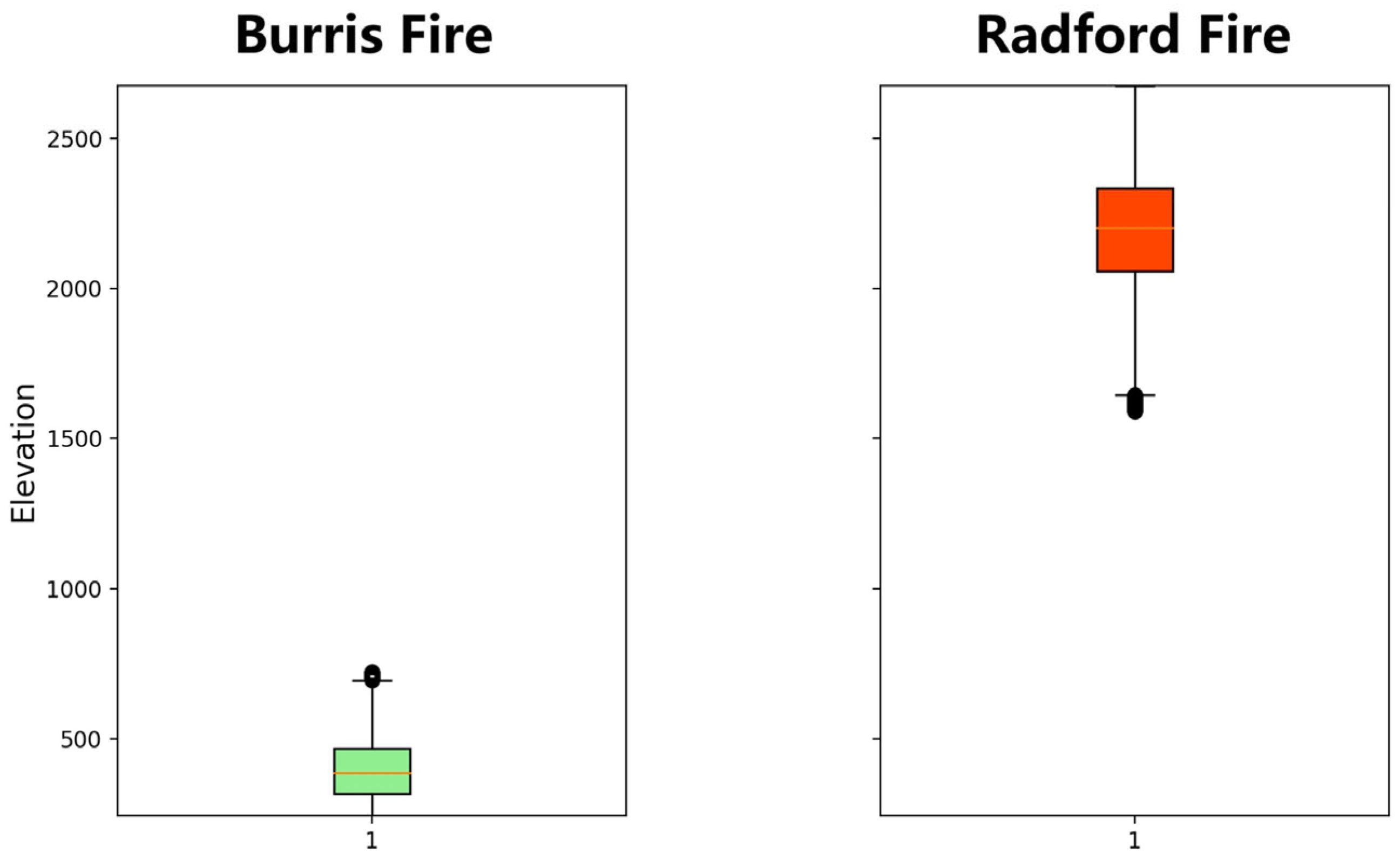
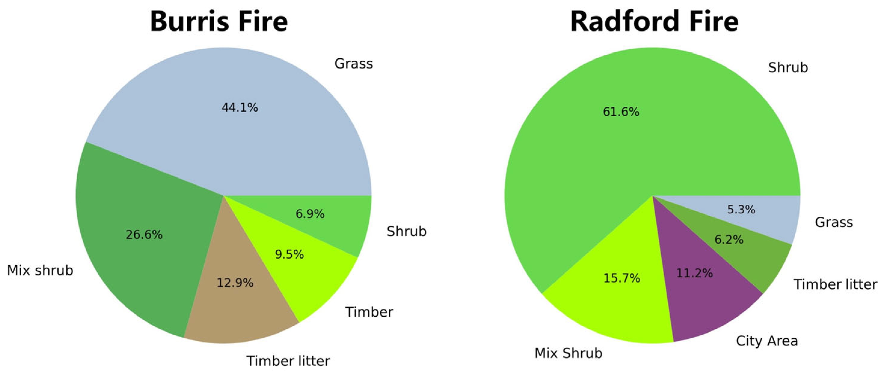
4.1. Comparison of Experimental Areas

We hope to summarize the impact of data absence on wildfire spread models from existing experiments, but the final results show that the impact of missing data attributes varies for different wildfire cases. Judgments need to be made based on the comprehensive geographical characteristics and real-time environmental factors of the experimental area, and there is no fixed impact pattern. Figure 6 shows the differences in elevation data and fuel models between the Burris Fire and the Radford Fire. It can be seen that the overall terrain of the Burris Fire is relatively flat, but there are many more hard-to-burn areas north of the ignition point (marked in gray), which makes the absence of elevation data have a smaller impact on model prediction, while the absence of the fuel model has a greater impact; the Radford Fire is located between mountains, with significant terrain undulations, but almost the entire study area is easily burnable. This geographical characteristic makes the sensitivity feature of data item absence completely opposite to that of Burris Fire, with the absence of the fuel model having a lesser impact on the model, and the absence of elevation data making the model prediction completely out of control. As for the absence of weather data, since our method of generating pseudo-data is to keep the initial values unchanged, its impact on the wildfire spread model will also depend on the initial values. From these experiments, we can also conclude that to infer the possible bias caused by different data absences, we should draw conclusions based on the local geographical characteristics, and there is still a lack of a fixed behavior pattern.

It is worth noting that although we have only selected two experimental areas, these regions are highly representative. Figure 7 and Figure 8 show the statistical distribution of elevation data and fuel models for the two study areas. It can be observed that the elevation of the Burris Fire is concentrated below 500 m and is extremely gentle, but it is filled with a large number of hard-to-burn areas (timber, etc.). In contrast, the Radford Fire is completely opposite, not only having extremely high altitudes but also being occupied by combustible materials (shrub) in most areas. Analyzing from the perspective of FARSITE’s operating principles, it can be seen that the factors influencing wildfire spread in these two regions are entirely different. The Burris Fire is due to the distribution of fuel, while the Radford Fire is due to elevation factors. Therefore, we can say that these two regions have a certain representativeness, as they can represent the absence of two key factors in FARSITE’s operation. However, our research still has certain limitations, and more universal cases are needed to explore specific behavioral patterns, which is also the direction of our future research.

4.2. Bias of Evaluation Metrics

In previous experiments, some experimental results showed an abnormal increase in evaluation metrics, which could not properly reflect the accuracy of the final prediction results. This sporadic phenomenon was actually caused by the computational characteristics of the evaluation parameters. The Jaccard coefficient, Sorensen metric, and Kappa statistics are based on the intersection over union (IoU) [26] to evaluate the similarity between the predicted fire perimeter and the actual fire perimeter. Figure 9 illustrates examples of good and bad accuracy using IoU; simply put, the results obtained by this calculation method are directly related to the proportion of the area where the predicted and recorded perimeters intersect. In the Radford Fire experiment, where there was an absence of elevation data as well as cases where both fuel and elevation data were missing, the final prediction yielded an almost circular result. This result accidentally overlapped significantly with the real fire scene, leading to anomalies in the Jaccard coefficient, Sorensen metric, and Kappa statistics. The intersection over the union method has been applied in various scenarios for assessing predictive error, and this phenomenon has led us to reconsider how to propose a more universal accuracy evaluation method in the context of wildfires.

The perimeter size differences, Sx, is a calculation method based on centroid size. Similarly, we also demonstrate an example of error calculation based on this method in Figure 10. It can be seen that when the predicted bounding box (orange) starts to move away from the centroid (ignition point), its centroid size is amplified, leading to an increased deviation. At the same time, since the centroid size is derived based on the Euclidean distance, we can summarize this method as a quantification of the similarity between two boundary shape curves, but it ignores the directionality of shapes. When two shapes are completely identical, the final error calculation results will not change, even if one of the shapes is rotated around the centroid. This can also explain why, in the Burris Fire experiment, all three scenarios of missing weather data resulted in a higher Sx. The absence of weather data led to the prediction that the wildfire would spread to the northeast, which is opposite to the actual recorded direction, but it happened to form a shape similar to the recorded boundary, resulting in an anomalous Sx. In the Radford Fire, where elevation data were missing, as well as in cases with both fuel and elevation data missing, the predicted area was smaller than the recorded boundary. This resulted in a final Sx greater than one, while in other cases, the predicted area was larger than the recorded boundary, leading to their Sx being less than one. This prevents intuitive comparisons and is a weakness of the Sx metric.

5. Conclusions

In this paper, we benchmarked the FARSITE model to simulate the impact of the missing data on wildfire spread prediction accuracy, considering the absence of weather, elevation, and fuel data. Experiments on two real wildfire cases revealed that certain parameters affect accuracy in specific scenarios, depending on the geographical characteristics of the study areas. The results suggest the need for tailored analysis based on local conditions.

The experiments also highlighted deficiencies in current metrics for assessing wildfire spread prediction accuracy. The Jaccard coefficient, Sorensen metric, Kappa statistics, and perimeter size differences have limitations in some extreme scenarios, failing to adequately indicate prediction quality. This finding underscores the challenge of developing more universally applicable assessment metrics.

The results provide crucial insights for decision-makers in real wildfire management, emphasizing the importance of assessing data completeness and accuracy when using predictive models. Incomplete or inaccurate data can lead to significant deviations in model predictions, potentially resulting in erroneous decisions and response measures if not carefully considered.

Future research will explore the specific impacts of data quality degradation on model predictive capabilities through more quantitative methods. By analyzing the role of different data types and their collective effect on prediction accuracy, we aim to uncover definitive patterns to guide adjustments of model parameters or strategies to minimize errors when data are missing or degraded. The ultimate goal is to develop more robust predictive tools that provide reliable guidance for effective wildfire management decisions in complex real-world situations.

References

1. Van der Werf, G.R.; Randerson, J.T.; Giglio, L.; van Leeuwen, T.T.; Chen, Y.; Rogers, B.M.; Mu, M.; van Marle, M.J.E.; Morton, D.C.; Collatz, G.J.; et al. Global Fire Emissions Estimates during 1997–2016. Earth Syst. Sci. Data 2017, 9, 697–720. [Google Scholar] [CrossRef]
2. Homepage|CIFFC. Available online: https://ciffc.ca/ (accessed on 21 March 2024).
3. Farsite, F.M. Fire Area Simulator-Model Development and Evaluation; Research Paper RMRS-RP-4 Revised; US Department of Agriculture, Forest Service, Rocky Mountain Research Station: Ogden, UT, USA, 2004. [Google Scholar]
4. Andrews, P.L.; Bevins, C.D.; Seli, R.C. BehavePlus Fire Modeling System, Version 4.0: User’s Guide; Gen. Tech. Rep. RMRS-GTR-106 Revised; Department of Agriculture, Forest Service, Rocky Mountain Research Station: Ogden, UT, USA, 2005; Volume 106, 132p. [Google Scholar]
5. Mandel, J.; Beezley, J.D.; Kochanski, A.K. Coupled Atmosphere-Wildland Fire Modeling with WRF 3.3 and SFIRE 2011. Geosci. Model Dev. 2011, 4, 591–610. [Google Scholar] [CrossRef]
6. Jiang, W.; Wang, F.; Fang, L.; Zheng, X.; Qiao, X.; Li, Z.; Meng, Q. Modelling of Wildland-Urban Interface Fire Spread with the Heterogeneous Cellular Automata Model. Environ. Model. Softw. 2021, 135, 104895. [Google Scholar] [CrossRef]
7. Jiang, W.; Qiao, Y.; Su, G.; Li, X.; Meng, Q.; Wu, H.; Quan, W.; Wang, J.; Wang, F. WFNet: A Hierarchical Convolutional Neural Network for Wildfire Spread Prediction. Environ. Model. Softw. 2023, 170, 105841. [Google Scholar] [CrossRef]
8. Benali, A.; Ervilha, A.R.; Sá, A.C.L.; Fernandes, P.M.; Pinto, R.M.S.; Trigo, R.M.; Pereira, J.M.C. Deciphering the Impact of Uncertainty on the Accuracy of Large Wildfire Spread Simulations. Sci. Total Environ. 2016, 569–570, 73–85. [Google Scholar] [CrossRef]
9. Cardil, A.; Monedero, S.; SeLegue, P.; Navarrete, M.Á.; de-Miguel, S.; Purdy, S.; Marshall, G.; Chavez, T.; Allison, K.; Quilez, R.; et al. Performance of Operational Fire Spread Models in California. Int. J. Wildland Fire 2023, 32, 1492–1502. [Google Scholar] [CrossRef]
10. Beven, K.; Binley, A. The Future of Distributed Models: Model Calibration and Uncertainty Prediction. Hydrol. Process. 1992, 6, 279–298. [Google Scholar] [CrossRef]
11. Thompson, M.P.; Calkin, D.E. Uncertainty and Risk in Wildland Fire Management: A Review. J. Environ. Manag. 2011, 92, 1895–1909. [Google Scholar] [CrossRef] [PubMed]
12. Yuan, X.; Liu, N.; Xie, X.; Viegas, D.X. Physical Model of Wildland Fire Spread: Parametric Uncertainty Analysis. Combust. Flame 2020, 217, 285–293. [Google Scholar] [CrossRef]
13. Cai, L.; He, H.S.; Liang, Y.; Wu, Z.; Huang, C. Analysis of the Uncertainty of Fuel Model Parameters in Wildland Fire Modelling of a Boreal Forest in North-East China. Int. J. Wildland Fire 2019, 28, 205–215. [Google Scholar] [CrossRef]
14. DeCastro, A.; Siems-Anderson, A.; Smith, E.; Knievel, J.C.; Kosović, B.; Brown, B.G.; Balch, J.K. Weather Research and Forecasting—Fire Simulated Burned Area and Propagation Direction Sensitivity to Initiation Point Location and Time. Fire 2022, 5, 58. [Google Scholar] [CrossRef]
15. Valero, M.M.; Jofre, L.; Torres, R. Multifidelity Prediction in Wildfire Spread Simulation: Modeling, Uncertainty Quantification and Sensitivity Analysis. Environ. Model. Softw. 2021, 141, 105050. [Google Scholar] [CrossRef]
16. Ciri, U.; Garimella, M.M.; Bernardoni, F.; Bennett, R.L.; Leonardi, S. Uncertainty Quantification of Forecast Error in Coupled Fire–Atmosphere Wildfire Spread Simulations: Sensitivity to the Spatial Resolution. Int. J. Wildland Fire 2021, 30, 790–806. [Google Scholar] [CrossRef]
17. GeoMAC Wildfire Application. Available online: https://wildfire.usgs.gov/geomac/GeoMACTransition.shtml (accessed on 20 December 2023).
18. LANDFIRE Program: Home. Available online: https://www.landfire.gov/ (accessed on 20 December 2023).
19. MesoWest Data. Available online: https://mesowest.utah.edu/ (accessed on 20 December 2023).
20. Radford Fire: 1088 Acres, 40% Contained. All Evacuation Orders Downgraded to Warnings—KESQ. Available online: https://kesq.com/news/2022/09/05/radford-fire-1088-acres-40-contained-all-evacuation-orders-downgraded-to-warnings/ (accessed on 20 December 2023).
21. You Searched for Burris Fire. The Mendocino Voice|Mendocino County, CA. Available online: https://mendovoice.com/search/burrisfire/ (accessed on 20 December 2023).
22. Lake County News, California—Search. Available online: https://lakeconews.com/component/%20search/ (accessed on 20 December 2023).
23. Arca, B.; Duce, P.; Laconi, M.; Pellizzaro, G.; Salis, M.; Spano, D. Evaluation of FARSITE Simulator in Mediterranean Maquis. Int. J. Wildland Fire 2007, 16, 563–572. [Google Scholar] [CrossRef]
24. Andrews, P.L. The Rothermel Surface Fire Spread Model and Associated Developments: A Comprehensive Explanation; United States Department of Agriculture, Rocky Mountain Research Station: Ogden, UT, USA, 2018. [Google Scholar]
25. Alexander, M.E.; Cruz, M.G. Evaluating a Model for Predicting Active Crown Fire Rate of Spread Using Wildfire Observations. Can. J. For. Res. 2006, 36, 3015–3028. [Google Scholar] [CrossRef]
26. Hao, Y. California Wildfire Spread Prediction Using FARSITE and the Comparison with the Actual Wildfire Maps Using Statistical Methods; University of California: Los Angeles, CA, USA, 2018. [Google Scholar]
27. Duff, T.J.; Chong, D.M.; Tolhurst, K.G. Indices for the Evaluation of Wildfire Spread Simulations Using Contemporaneous Predictions and Observations of Burnt Area. Environ. Model. Softw 2016, 83, 276–285. [Google Scholar] [CrossRef]
28. Duff, T.J.; Chong, D.M.; Taylor, P.; Tolhurst, K.G. Procrustes Based Metrics for Spatial Validation and Calibration of Two-Dimensional Perimeter Spread Models: A Case Study Considering Fire. Agric. For. Meteorol. 2012, 160, 110–117. [Google Scholar] [CrossRef]
29. Filippi, J.-B.; Mallet, V.; Nader, B. Representation and Evaluation of Wildfire Propagation Simulations. Int. J. Wildland Fire 2013, 23, 46–57. [Google Scholar] [CrossRef]
Figure 1. The real wildfire Burris Fire.
Fire 07 00141 g001
Figure 2. The real wildfire Radford Fire.
Fire 07 00141 g002
Figure 3. Pseudo-data generation process.
Fire 07 00141 g003
Figure 4. Experimental results on Burris Fire.
Fire 07 00141 g004
Figure 5. Experimental results on Radford Fire.
Fire 07 00141 g005
Figure 6. Comparison of Burris Fire and Radford Fire on the elevation data and fuel model(the blue border refers to the record fire perimeter.).
Fire 07 00141 g006
Figure 7. Statistical comparison of the elevation data.
Fire 07 00141 g007
Figure 8. Statistical comparison of the fuel model.
Fire 07 00141 g008
Figure 9. Examples of error calculation methods based on intersection over union.
Fire 07 00141 g009
Figure 10. Examples of error calculation methods based on centroid size.
Fire 07 00141 g010