Abstract
Wildfire activity in the western United States has been on the rise since the mid-1980s, with longer, higher-risk fire seasons projected for the future. Prescribed burning mitigates the risk of extreme wildfire events, but such treatments are currently underutilized. Fire managers have cited lack of firefighter availability as a key barrier to prescribed burning. We use both principal component analysis (PCA) and logistic regression modeling methodologies to investigate whether or not (and if yes, under what conditions) personnel shortages on a given day are associated with lower odds of a prescribed burn occurring in the Okanogan–Wenatchee National Forest. We utilize the logit model to further assess how personnel availability compares to other potential barriers (e.g., meteorological conditions) in terms of association with odds of a prescribed burn occurring. Our analysis finds that fall and spring days in general have distinct constellations of characteristics. Unavailability of personnel is associated with lower odds of prescribed burning in the fall season, controlling for meteorological conditions. However, in the spring, only fuel moisture is observed to be associated with the odds of prescribed burning. Our findings suggest that if agencies aim to increase prescribed burning to mitigate wildfire risk, workforce decisions should prioritize firefighter availability in the fall.
1. Introduction
Wildfires pose an increasing risk to the western United States due to a complex interacting set of factors, including climate change, increased population in the wildland urban interface, and long-term fire suppression policies resulting in the buildup of fuels. These factors have been associated with increased wildfire activity and severity as well as projected continuing impacts such as longer, higher-risk, and higher-impact fire seasons, with historically rare wildfire events becoming more frequent [1,2,3]. Considering the increasing likelihood of severe wildfire events, the implementation of risk management strategies is critical. Fuel treatment, and in particular prescribed burning, has proven to reduce the risk of extreme fire events through the reduction of fuels; however, prescribed burns are underutilized at present [4]. It is important to understand the barriers in order to consider what steps are needed to facilitate an increase in future prescribed burning. Land and fire managers have cited numerous barriers to prescribed burning, such as personnel shortages, lack of funding, and narrow burn windows, as well as smoke impacts and environmental regulations [5,6,7,8,9].
This work explores the quantitative evidence base in support of earlier qualitative reports and findings, specifically the expressed perception among fire managers that personnel unavailability (due to prior deployment of firefighters for wildfire suppression or other purposes) is a significant barrier to prescribed burning. Given the variability in conditions and burning processes across forests, we adopt a case study approach focused on the Okanogan–Wenatchee National Forest. This research was done in partnership with the US Forest Service (USFS) as part of a larger co-production effort related to the management of risk associated with simultaneous and impactful wildfires in the US [3]. Our analysis addresses the following specific research questions: (1) Is personnel unavailability on a given day associated with lower odds of a prescribed burn occurring in the Okanogan–Wenatchee National Forest? (2) If yes, under what conditions? (3) If personnel unavailability is associated with lower odds of a prescribed burn occurring, how does this compare to other potential barriers (such as meteorological conditions)? We hypothesize that there is a relationship between personnel unavailability and the odds of a prescribed burn being conducted on a given day.
Wildfire activity in the western US began to increase sharply in the mid-1980s, and fire seasons have continued to intensify over recent decades [1,10,11]. Three key factors found to be contributing to the intensification of fire seasons are (1) changing climate; (2) changes in human settlement, with more people living in the wildland–urban interface; and (3) decades of fire suppression, leading to a buildup of fuels [1,4,11,12]. Climate models project longer seasons of simultaneous wildfires in the future, which has implications for competition for response resources and firefighting effectiveness [13]. Ignition precursors are associated with projected levels of personnel demand and deployment, and decisions about response resources must take simultaneous demand into consideration [13]. The increased resource demand observed over the last two decades is partially attributable to increases in simultaneous wildfire [13]. This suggests that we are likely to see increasing demand and competition for firefighting resources in the future.
Land management agencies in the US have relied heavily on policies of fire suppression, due to agencies’ aversion to short-term risk and smoke impacts. However, fire suppression increases the risk of more severe wildfire in the long-term due to the buildup of fuels. There is strong evidence that fuel reduction treatments, such as prescribed burning, are highly effective at mitigating the risk of high-severity fires [4,12]. The current use of prescribed burning is insufficient to address the level of fuel buildup; thus, there is a dire need for increased pace and scale. Prescribed burning is a perennial necessity in fire-adapted landscapes [4]. Still, land managers face challenging forest management decisions and must confront tradeoffs when opting for wildfire risk mitigation strategies, such as prescribed burning. A case study analysis of the Upper Wenatchee Pilot Project, which considered treatment alternatives in the Okanogan–Wenatchee National Forest, demonstrated that land managers could benefit from employing a decision analysis framework to evaluate the tradeoffs of different treatment options [14].
Considering the strong scientific evidence that prescribed burning is an effective but underutilized wildfire risk mitigation strategy, it is important to understand the barriers precluding land managers from conducting burns. Past studies investigating the barriers to prescribed burning using qualitative methods have explored potential barriers, including resource capacity (i.e., funding and personnel), narrow burn windows, and environmental impacts and regulations, as well as liability concerns. These studies have identified lack of resources (including insufficient available firefighters) as a key barrier to prescribed burning across regions in the United States [5,6,7,8,9]. In fact, the most cited barrier to prescribed burning among federal and state land managers in the western US was lack of adequate funding and capacity, including resources, knowledge, and people to conduct the work. Specifically, land managers reported that personnel are frequently unavailable due to the demands of wildfire suppression activities [7]. Additional qualitative studies corroborate these expressed perceptions, as a survey of district-level fire managers in northern California identified lack of adequate personnel as a significant hurdle to prescribed burning [5], and key participants in California’s prescribed burn policy conversations stated that limited burn crew availability restricts when and where prescribed burns can occur [8]. Fire use practitioners in the southern US [6] and in the mid-Atlantic region [9] similarly identified resource capacity (including staffing) as a barrier to prescribed burning.
While there are numerous qualitative studies investigating barriers to prescribed burning through survey research and other qualitative methods, the use of quantitative data and analysis to support these studies is a gap in the literature. Specifically, to our knowledge, no studies have taken a quantitative approach to determining whether or not and under what conditions personnel unavailability is a barrier to prescribed burning. The objective of this study is to use quantitative methods to analyze the relationship between personnel unavailability and the occurrence of prescribed burning. We seek to determine whether or not observed data support fire managers’ assertions that a lack of firefighter availability thwarts prescribed burns. First, we use principal component analysis (PCA) [15] to explore the key metrics that characterize the days when prescribed burning does and does not occur. Second, we use logistic regression modeling [16] to analyze whether or not personnel unavailability is associated with lower odds of a prescribed burn occurring. Our goal is to gain a better understanding of the relationship between the firefighter resource and prescribed burning in order to support USFS decisions about budgets, hiring, and personnel retention.
2. Materials and Methods
2.1. Data
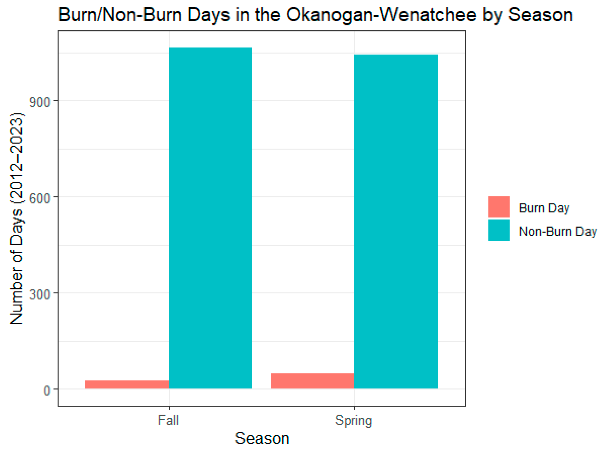
We rely on several datasets for this study. First, our outcome variable, whether or not a prescribed burn occurred in the Okanogan–Wenatchee National Forest on a given day, is extracted from the US Forest Service’s Natural Resource Manager (NRM) Forest Activity Tracking System (FACTS) [17]. Within FACTS, the hazardous fuel treatment reduction dataset includes all reduction activities across the United States. We filter the data to include all fuel treatments in the Okanogan–Wenatchee National Forest designated as prescribed burns, with the activity specified as broadcast burn or underburn. In addition, we restrict the dataset to burns between 2012 and 2023 to align with data availability for other variables. We filter the data for season, distinguishing spring (March/April/May) from fall (September/October/November), using a dummy variable (Spring/Fall, with Spring = 1). We remove days from 20–31 May 2022 from the dataset, because US Forest Service Chief Randy Moore implemented a 90-day ban on prescribed burning on 20 May 2022. This results in 121 burns across 77 distinct burn days. The number of burn/non-burn days in the dataset is summarized by season in Figure 1.
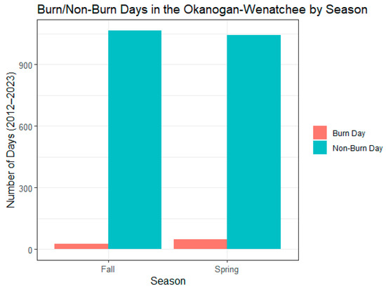
Figure 1.
Bar chart of the number of days with and without prescribed burns in fall/spring from 2012 to 2023.
The prescribed burn dates in FACTS are manually entered into the record and thus can be imprecise. For this reason, we considered instead using the VIIRS (Visible Infrared Imaging Radiometer Suite) dataset, which uses a satellite to detect fires. Unfortunately, however, about a quarter of the prescribed burns reported in FACTS are missing in the VIIRS data, likely due to factors such as cloud cover or the timing of the satellite passing overhead. This precludes simply using VIIRS for our analysis as this would result in many recorded prescribed burns being omitted. Given this issue, we chose to use FACTS data for the analyses presented in the main body of this paper. For comparison, we also re-ran our analyses using data from VIIRS (where available) and found generally similar results (see Appendix C). This supports a conclusion that any imprecision in the dates entered in FACTS may introduce noise into the analysis but ultimately does not bias the results.
Second, fuel moisture data are compiled from gridMET [18], a high-resolution spatial dataset of surface meteorological variables across the contiguous US. GridMET uses interpolation to combine climate data from PRISM with temporal attributes from regional reanalysis (NLDAS-2). Data are available on a 4 km grid. We restrict the dataset to the Okanogan–Wenatchee National Forest and compute the mean 100 h fuel moisture (FM100) and the mean 1000 h fuel moisture (FM1000) for each fall and spring day from 2012 to 2023. In addition, daily smoke ventilation index data are generated from ERA5 for a representative location, 48.25 N, 121.25 W, at time 22Z, applying mixing height and transport wind [19]. The mixing height is calculated by employing two-meter air temperature and assuming adiabatic rise until intersection with the environmental lapse rate.
We utilize data from the US Incident Management Situation Reports (IMSRs) for the national and Northwest Interagency Coordination Center (NWCC) preparedness levels (PLs) and the number of acres of active wildfire within the NWCC each day [20]. Preparedness levels reflect suppression readiness and firefighting resource demand and are defined using multiple factors. These include weather conditions, expected fire activity, and resource availability [21]. Preparedness levels are set daily at both the national and regional levels. We consider national and NWCC PLs and the acres of active wildfire within the NWCC as part of our model approach, because these factors are expected to interact with decisions about prescribed burning.
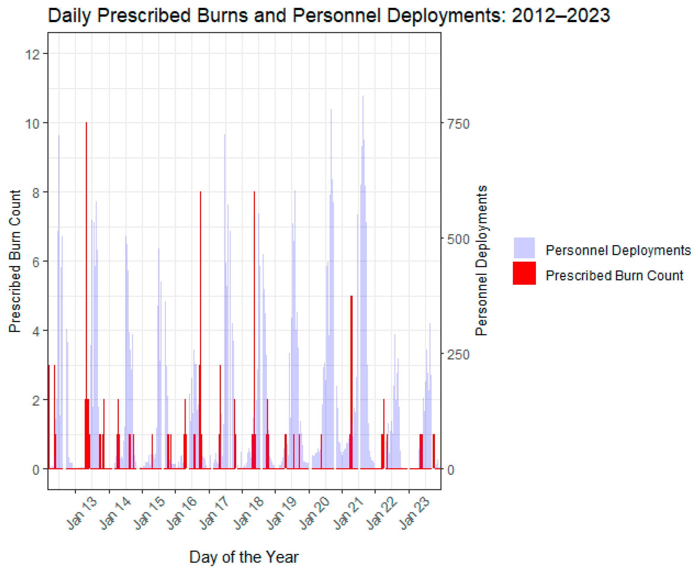
Finally, personnel assignment data are pulled from the Resource Ordering and Status System (ROSS; 2012–2019) and the Interagency Resource Ordering Capacity (IROC; 2020–2023) [22,23]. The ROSS/IROC database tracks the personnel requests and deployments for wildfire incidents across the US [24]. Personnel are hired by multiple agencies for multiple purposes, and the workforce available for deployment fluctuates throughout the year. Although some firefighters are full-time employees, additional seasonal workers are also hired, typically from early May to late September [25]. The total number of personnel in the workforce at any given time is not tracked, so the total number of personnel deployed serves as a proxy for resource availability. We calculate the number of personnel currently deployed to estimate the number of personnel unavailable for prescribed burning management on a given day. Specifically, we consider personnel from the Okanogan–Wenatchee National Forest, personnel from other national forests in Washington, and Washington state personnel. We aggregate the counts of Crew, Air, Equipment, and Overhead personnel deployed from these three resources to compute a total number of unavailable personnel for each day, as shown in Figure 2. The number of unavailable personnel differs between seasons, as well as between burn days and non-burn days, as shown in Figure 3. There are many more unavailable personnel, on average, in the fall than in the spring.
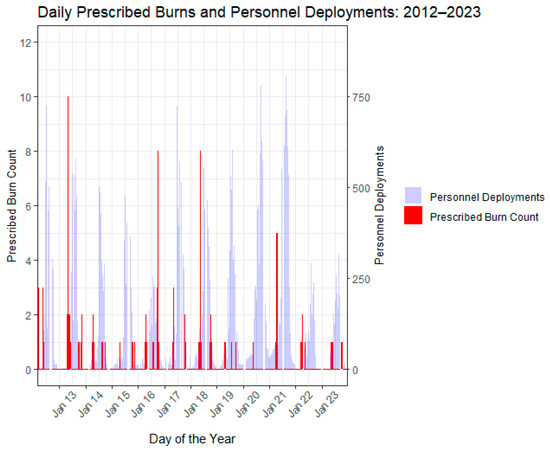
Figure 2.
Histogram of daily prescribed burn count and number of personnel deployed from 2012 to 2023. Red bars indicate number of prescribed burns on a given day (left hand axis). Purple bars represent number of personnel unavailable (right hand axis).
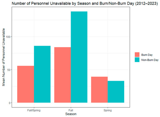
Figure 3.
Comparison of number of unavailable personnel on burn days versus non-burn days (2012–2023) clustered by season.
See Table 1 for a summary of the data used for each variable. Summary statistics for all variables are included in Appendix A.

Table 1.
Summary of each variable used in the analysis and the corresponding data source.
2.2. Methods
We explore our research question using principal component analysis (PCA) and a logistic regression model. The outcome we are interested in is whether or not a prescribed burn occurs on a given day, while the independent variables we consider are the number of unavailable personnel (i.e., personnel already deployed), the number of acres of active wildfire in the NWCC, the national PL, the NWCC PL, season (spring versus fall), fuel moisture (FM100 and FM1000), and smoke ventilation index, with subsets incorporated for each method as appropriate. The unit of analysis is a day.
- Principal Component Analysis (PCA)
We conduct PCA to explore the dominant modes that characterize days with and without prescribed burns and distill the subset of variables observed to be most associated with whether or not a prescribed burn happens on a given day. For each day in the dataset, we include the number of unavailable personnel, i.e., personnel currently deployed and thus not available for assignment; the season (spring or fall); the number of acres of active wildfire in the NWCC; the national PL; the NWCC PL, FM100, FM1000; and the ventilation index. We consider both burn days and non-burn days, and we explore whether or not days with different burn statuses and in different seasons are associated with different levels of unavailable personnel and other independent variables. Although we recognize that PL is a categorical variable in practice, we treat PL as a numeric variable in order to include it in the analysis.
We present results from the analysis of spring and fall days combined. PCA applied to spring, summer, and fall days, and also separate analyses restricted to only spring and only fall days, are included in Appendix B.
- 2.
- Logistic Regression Model
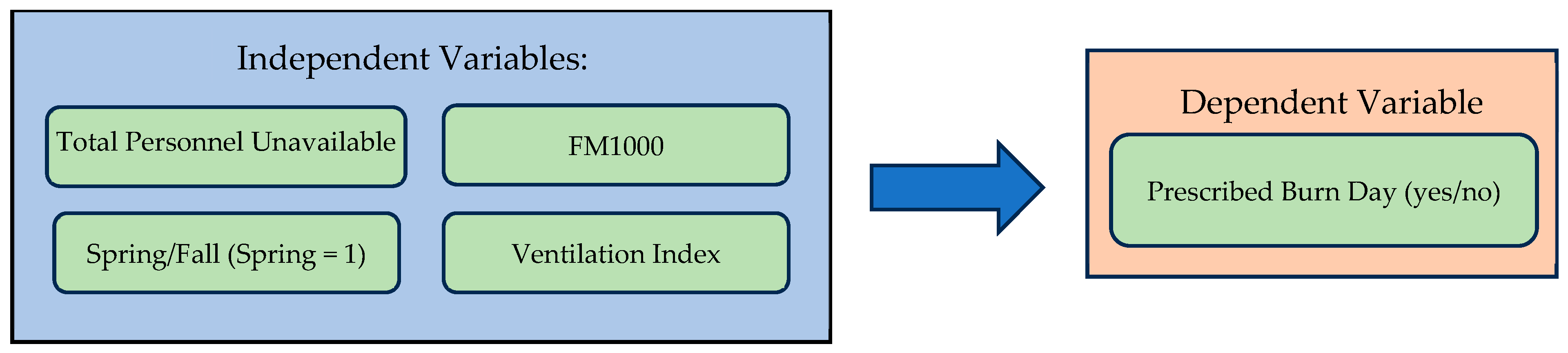
In addition, we develop a logistic regression model to estimate the odds of a prescribed burn occurring on a given day. We fit the model on fall and spring days combined, and additionally on fall and spring days separately. We use AIC to compare the fit between models. The dependent variable is binary, indicating whether a prescribed burn occurs or not. The logit model includes the following independent variables: the number of unavailable personnel, the season, FM1000, and ventilation index. The flowchart in Figure 4 below summarizes the model:

Figure 4.
Flow chart of the logit model used to estimate the odds of a prescribed burn occurring on a given day.
The coefficient (β), associating each independent predictor variable with the outcome, is estimated. The percent change in the odds of a given day being a burn day, associated with a one-unit shift in the value of the predictor variable, is then assessed as (exp(β) − 1) ∗ 100. We note that, although the PLs, acres of active wildfire in the NWCC, and FM100 (all included in the PCA) may also be associated with whether or not a prescribed burn occurs, these variables are highly correlated with the other independent variables included in the model. For this reason, and given the small number of prescribed burning days in our dataset, we elect to construct a parsimonious logit design. The relationship between fuel moisture and the odds of a prescribed burn is complex, because fuels need to be sufficiently dry for a prescribed burn to work, while being not too dry that there is a high risk of wildfire. This suggests a non-linear relationship between fuel moisture and the odds of a prescribed burn, so we fit the logit model to include both fuel moisture alone and a quadratic term for fuel moisture. We also fit parallel analyses that include interaction terms, but we did not find that this improves the fit, so we did not ultimately include interactions in the model. The mathematical formulations of the models that we fit are included below; the dummy variable for Spring/Fall (Spring = 1) is only relevant when we fit the models on fall and spring days combined.
Quadratic:
Linear:
3. Results
3.1. Principal Component Analysis (PCA)
3.1.1. Burn and Non-Burn Days (Spring and Fall)
In the analysis of all spring and fall days (2012–2023), the PCA resolves a substantial amount of the variance in the dataset. We find that the first principal component (PC1) accounts for approximately 52 percent of the variance and PC2 accounts for approximately 18 percent (see Table 2 and Figure 5). This suggests that the dimension reduction is effective in accounting for variance. Visual inspection of Figure 5 reveals that burn days (indicated by the black markers) are less likely to be days with relatively high numbers of unavailable personnel (indicated by the larger markers) and that burn days appear in a narrow band of PC1 values.
Table 2.
Principal component analysis for all days in fall and spring (2012–2023). Proportion of variance explained by each of the first four PCs, and loadings for each variable on each PC, are displayed.

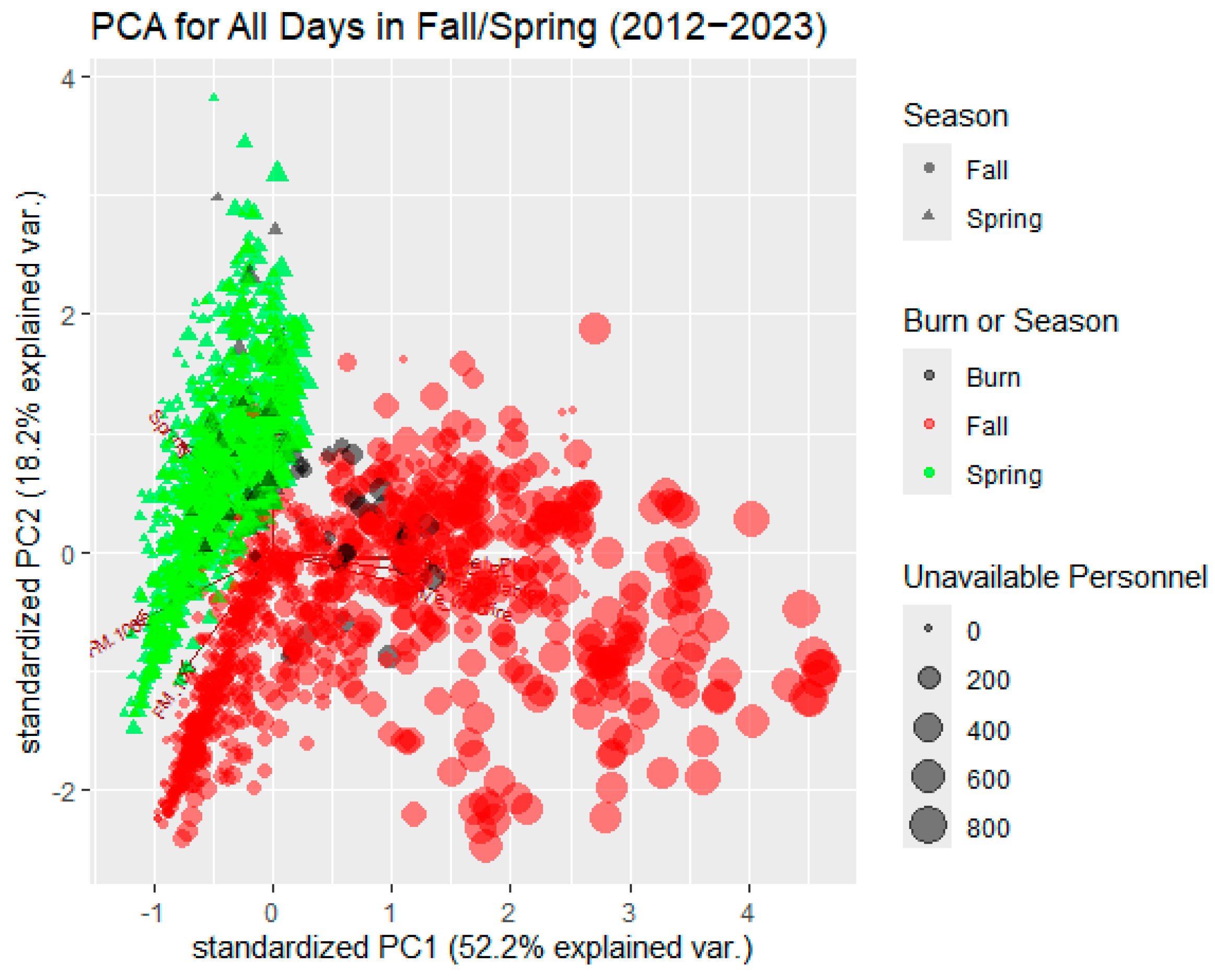
Figure 5.
Plot of PC2 vs. PC1 for all days in the fall and spring (2012–2023). Each marker represents one day. Fall days are represented by circular markers, while spring days are represented by triangular markers. Green represents spring days on which no prescribed burn occurs, red represents fall days on which no prescribed burn occurs, and black represents prescribed burn days. Marker size indicates the number of unavailable personnel recorded for each day.
PC1 is characterized by a strongly positive weighting on the national PL, followed closely by the NWCC PL, number of unavailable personnel, and acres of active wildfire, also with positive associations. FM1000, FM100, and the spring season are negatively associated with PC1, although at lower weights, indicating that wetter fuels and spring days are associated with lower values of PC1. The fact that burn days fall into a relatively narrow range of lower values of PC1 indicates that burn days tend to have lower numbers of personnel unavailable, lower PLs, and less active wildfire, although differences are evident by season.
In PC2, the ventilation index and the spring season are weighted positively. By contrast, FM1000, FM100, and acres of active wildfire have negative weights, while the number of personnel unavailable, national PL, and NWCC PL are only minimally weighted. The visual inspection of burn days (the black markers in Figure 5) indicates that prescribed burn days span a relatively wide range of PC2 values.
We observe in Figure 5 that days cluster by season. The fall days map onto relatively higher values of PC1, which indicates an association with higher national and NWCC PLs, more unavailable personnel, drier fuels, and more acres of active wildfire. Spring days map onto lower values of PC1, indicating an association with wetter fuels, lower national and NWCC PLs, fewer unavailable personnel, and fewer acres of active wildfire. Spring days are concentrated in a narrow range between –1 and 0 in PC1, while fall days range from –1 to 4. This suggests that the conditions characterizing fall days are more variable, particularly in terms of the number of unavailable personnel, acres of active wildfire, and PLs (i.e., the variables more heavily weighted in PC1). The differences between fall and spring days are less stark in PC2, with fall days mapping onto lower values on average. The characteristics of burn days by season are complex and warrant further exploration, as detailed below.
3.1.2. Burn Days (Spring and Fall)
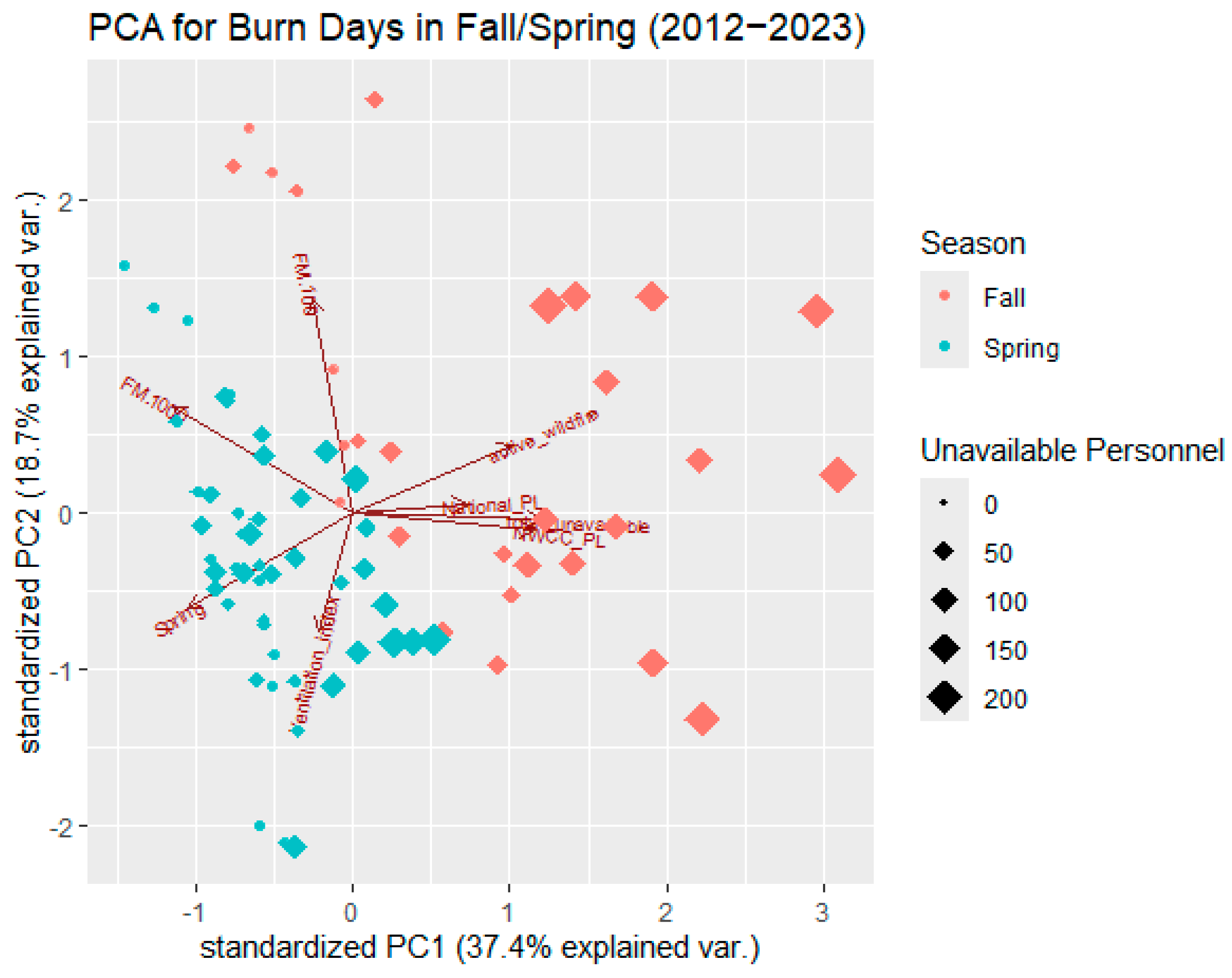
Filtering the dataset for days on which prescribed burns occurred (i.e., the black markers in Figure 5), we carry out PCA on this subset and observe that PC1 accounts for approximately 37% of the variance and PC2 accounts for nearly 19% of the variance (see Table 3 and Figure 6). This suggests that the dimension reduction approach is effective in characterizing common modes and identifying distinguishing features within the burn day subset.
Table 3.
Principal component analysis for burn days in fall and spring (2012–2023). Proportion of variance explained by each of the first four PCs, and loadings for each variable on each PC, are displayed.
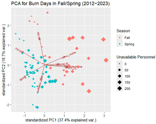
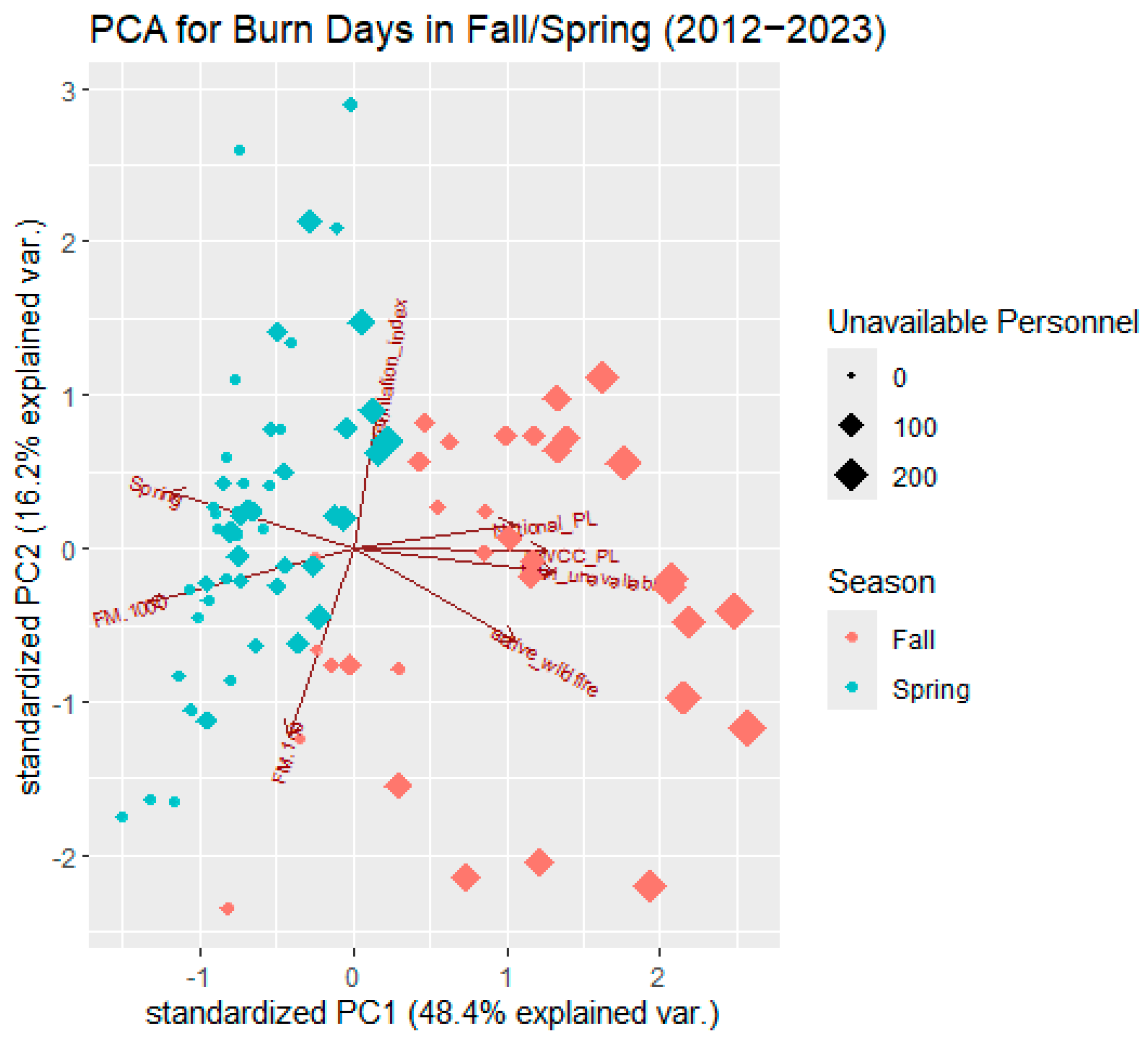
Figure 6.
Plot of PC2 vs. PC1 for burn days in the fall and spring (2012–2023). Each marker represents one day. Season is distinguished by color (fall by red marker, spring by blue marker). Marker size indicates the number of unavailable personnel recorded for each day.
Delving into the statistical results, we find rich and complex associations with burn days. The number of unavailable personnel is heavily positively weighted in PC1, indicating a strong association between personnel unavailability and the characterization of burn days, with higher levels of unavailability on a given day resulting in higher values of PC1. Acres of active wildfire and higher national and NWCC PLs are also positively associated with PC1, while FM1000 and the spring season are strongly negatively weighted. FM100 and ventilation index are also negatively loaded in PC1, but these variables have relatively little weight. This indicates that the number of unavailable personnel, acres of active wildfire, PLs, FM1000, and spring season are all important in characterizing burn days, as expressed in PC1.
In PC2, FM100 is positively associated and has the heaviest weight, indicating that fuel moisture leads to higher values of PC2 and fuel moisture is important in characterizing burn days. FM1000 and acres of active wildfire are similarly positively associated. Ventilation index and the spring season are negatively weighted, indicating that increases in smoke ventilation and days falling in spring are associated with lower values of PC2. National and NWCC PLs and the number of personnel unavailable all have relatively small weights in PC2, indicating that the impact of these variables is already captured by PC1.
A visual inspection of Figure 6 reveals that burn days form clusters by season, just as in the analysis of all days (burn days and non-burn days). The fall days tend to associate with higher values of PC1, while the spring days tend to associate with lower values. Thus, fall burn days are associated with more unavailable personnel, higher national and NWCC PLs, more acres of active wildfire, and drier fuels. Spring burn days are associated with wetter fuels, slightly higher ventilation indices, lower national and NWCC PLs, fewer unavailable personnel, and less active wildfire. Fall and spring burn days both span a wide range of values of PC2.
In summary, the PCA findings contribute to the evidence confirming visual impressions that prescribed burns do not tend to occur on days with higher numbers of personnel unavailable. Personnel unavailability is an important variable for characterizing burn days, and burn days are associated with lower numbers of unavailable personnel, while other variables also contribute to the overall picture.
3.2. Logistic Regression Model
Logistic regression (logit) results assessing the association of our input variables with the odds that prescribed burning will occur on a given day are presented in Table 4. We consider models that include fuel moisture as a linear term and as a non-linear (quadratic) term.
Table 4.
Logistic regression results for prescribed burning in the fall, spring, and fall/spring.
3.2.1. Fall Days
Analyzing fall days, our logit model finds that the number of unavailable personnel and the fuel moisture are statistically significantly associated with the odds of a prescribed burn occurring on a given day, while the ventilation index is not. The logit model, including fuel moisture as a non-linear term, is a much better fit for the data.
There are 1092 fall days in the dataset, with a prescribed burn occurring on 28 of those days. Thus, the overall odds of a prescribed burn occurring on a fall day are 0.026. We find that one additional personnel member being unavailable is associated with an expected 0.40% decrease in the odds of a day being a prescribed burn day, holding fuel moisture and ventilation index constant. Another way to express this result is that an additional eighteen-person crew being unavailable is associated with an expected 6.95% decrease in the odds of a day being a prescribed burn day. The marginal effect of a one percent increase in FM1000 (i.e., wetter fuel) depends on the starting value of fuel moisture, because fuel moisture is included as a non-linear term in the model. One way to conceptualize how the effect of fuel moisture changes as the starting value of fuel moisture changes is to consider the marginal effect at representative values, i.e., at the mean, two standard deviations below the mean, and two standard deviations above the mean. At the mean fuel moisture in the fall (18.29%), a one percent increase in FM1000 is associated with a nearly 23% decrease on average in the odds of a day being a prescribed burn day, holding the number of unavailable personnel and ventilation index constant. Two standard deviations below the mean fuel moisture in the fall (a fuel moisture of 6.65%), a one percent increase in FM1000 is associated with a 186% increase on average in the odds of a day being a prescribed burn day. Finally, two standard deviations above the mean fuel moisture in the fall (29.92%), a one percent increase in FM1000 is associated with a 79% decrease on average in the odds of a day being a prescribed burn day. The ventilation index does not have a statistically significant effect on the odds of a prescribed burn in the fall (p = 0.4519).
3.2.2. Spring Days
For spring days, our logit model finds a statistically significant association only between fuel moisture and the odds of a prescribed burn occurring on a given day, while neither the number of personnel unavailable nor the ventilation index is statistically significant. The logit model for spring days that includes fuel moisture only as a linear term also finds the ventilation index to be modestly statistically significantly associated with the odds of a prescribed burn occurring on a given day. However, similarly to the fall, the logit model including a quadratic term for fuel moisture is a better fit.
There are 1092 spring days in the dataset, and a prescribed burn occurred on 48 of those days. Therefore, the overall odds of a prescribed burn occurring on a spring day are 0.047. The marginal effect of a one percent increase in FM1000 (i.e., wetter fuel) depends on the starting value of fuel moisture. At the mean fuel moisture in the spring (21.31%), a one percent increase in FM1000 is associated with an 18.5% decrease on average in the odds of a day being a prescribed burn day, holding the number of unavailable personnel and ventilation index constant. Two standard deviations below the mean fuel moisture in the spring (12.66%), a one percent increase in FM1000 is associated with a 95.9% increase on average in the odds of a day being a prescribed burn day. Finally, two standard deviations above the mean fuel moisture in the spring (29.96%), a one percent increase in FM1000 is associated with a 66% decrease on average in the odds of a day being a prescribed burn day.
3.2.3. Combined Fall and Spring Days
Similarly to the result for spring days, our logit model for fall and spring days (combined) finds a highly statistically significant association between fuel moisture and the odds of a prescribed burn occurring on a given day. The ventilation index is modestly statistically significantly associated with the odds of a prescribed burn occurring on a given day. The logit model for fall and spring days that includes fuel moisture only as a linear term finds the number of unavailable personnel, the season (fall relative to spring as the reference category), fuel moisture, and ventilation index all to be statistically significantly associated with the odds of a prescribed burn occurring on a given day. However, the logit model that allows for a non-linear relationship between fuel moisture and the odds of a prescribed burn on a given day is a much better fit (see Table 4 for AIC values). Once the quadratic fuel moisture term is added, the number of unavailable personnel and the season (fall relative to spring as the reference category) lose statistical significance.
There are 2184 spring and fall days in the dataset, and 77 of those are prescribed burn days. So, the overall odds of a prescribed burn occurring on a fall/spring day are 0.0365. Again, the marginal effect of a one percent increase in FM1000 (i.e., wetter fuel) varies depending on the starting level of fuel moisture. At the mean fuel moisture (19.8%), a one percent increase in FM1000 is associated with a nearly 16% decrease on average in the odds of a day being a prescribed burn day, holding the number of unavailable personnel, season, and ventilation index constant. Two standard deviations below the mean fuel moisture (9.11%), a one percent increase in FM1000 is associated with an 80% increase on average in the odds of a day being a prescribed burn day. Finally, two standard deviations above the mean fuel moisture (30.49%), a one percent increase in FM1000 is associated with a nearly 61% decrease on average in the odds of a day being a prescribed burn day. A one unit increase in the ventilation index is associated with a 0.007% decrease on average in the odds of a day being a prescribed burn day, holding the number of unavailable personnel and fuel moisture constant.
4. Discussion
Our research questions and hypotheses were motivated by earlier qualitative survey results in which fire operations staff indicated that lack of available personnel is a barrier to prescribed burning [5,6,7,8,9]. Specifically, our research questions are as follows: (1) Is personnel unavailability on a given day associated with lower odds of a prescribed burn occurring in the Okanogan–Wenatchee National Forest? (2) If yes, under what conditions? (3) If personnel unavailability is a barrier, how does this compare to other potential barriers? Our results provide quantitative evidence to support these qualitative findings under specific conditions for the Okanogan–Wenatchee National Forest. Specifically, all of our analytical approaches find that there are strong seasonal differences between fall and spring, and the relationship between personnel availability and prescribed burning is significant only for fall. Past survey research did not discuss the potential impact of season on the relationship between personnel availability and prescribed burning.
PCA reveals that the days in the dataset can largely be characterized by two components: the first pertains to factors related to personnel availability and the second pertains to meteorological conditions. In the PCA for all days (burn and non-burn), the variables most closely related to the deployment of personnel (PLs and number of unavailable personnel) characterize PC1 and thus explain the largest share of overall variability, while the meteorological variables (ventilation index, the spring season, and fuel moisture) characterize PC2. These first two principal components are orthogonal by definition but certainly interact to some extent. For example, acres of active wildfire in the NWCC weighs significantly on both PCs, but the division between variables related to personnel deployment and meteorological variables is the most salient feature. Looking specifically at burn days, we find that these tend to fall into a narrow range of low values in the first principal component, while the range of values for the second principal component is relatively wide. These results indicate that the dominant characteristics distinguishing burn days are lower numbers of personnel unavailable and lower PLs, while burn days are not necessarily distinguished by the specific meteorological conditions represented in our dataset. Additionally, when the dataset is restricted to burn days, we observe that the range of the number of unavailable personnel from the Okanogan–Wenatchee National Forest, other national forests in Washington, and Washington state personnel tops out around 200 persons, while the number of unavailable personnel reaches levels of about 800 persons when looking across all days.
This analysis clearly reveals differences associated with season. Although both fall and spring are considered prescribed burn seasons, we find that more prescribed burns occur in the spring, which is also the season during which there are fewer unavailable personnel. Of the 77 prescribed burn days in the dataset, 49 were in the spring. Moreover, the mean number of unavailable personnel on a spring day is around 33 persons, while the mean number of unavailable personnel on a fall day is around 136 persons. PCA for all days (burn and non-burn), and also for burn days alone, reveals that fall days are associated with more personnel being unavailable, higher PLs, more acres of active wildfire, and drier fuels. Spring days overall are associated with wetter fuels, lower PLs, fewer unavailable personnel, and less active wildfire.
Moreover, we find evidence that the number of unavailable personnel is significantly associated with the odds of a prescribed burn occurring on a given day in the fall, but not in the spring. In the fall, we find strong evidence of a relationship between the number of unavailable personnel and the odds of a prescribed burn occurring on a given day. We note that there are many additional factors that contribute to prescribed burning decisions, including meteorological conditions and, in particular, potential smoke impacts. Nonetheless, holding fuel moisture and ventilation index (two key indices for meteorological conditions for burning) constant, our logit model shows that an increase in the number of unavailable personnel is associated with a decrease in the odds of a prescribed burn on a fall day. This supports fire managers’ statements that lack of firefighter availability is a barrier to prescribed burning.
However, as mentioned above, this relationship does not hold in the spring. Holding fuel moisture and ventilation index constant, our logit model does not find a relationship between the number of unavailable personnel and the odds of a prescribed burn day in the spring.
Our analysis finds that fuel moisture is the only variable that has a consistent relationship with the odds of a prescribed burn across seasons. In both fall and spring, on average, low levels of fuel moisture (i.e., drier fuels) are associated with an increase in the odds of a prescribed burn day, average levels of fuel moisture are associated with a decrease in the odds of a prescribed burn day, and high levels of fuel moisture (i.e., wetter fuels) are associated with a substantial decrease in the odds of a prescribed burn day.
Although prior survey research on seasonal differences between fall- and spring-prescribed burns is sparse, there is evidence of seasonal differences in other literature. Prescribed burn windows are known to vary by season [26], and there are ecological differences between fall- and spring-prescribed burning conditions. In the spring, prescribed burning occurs as surface fuels are drying, while fall-prescribed burns tend to occur after the first rains have moistened fuels [27]. Fall fuels are typically drier, burn at higher temperatures, and have more complete combustion, relative to spring fuels [28]. Moreover, a study of the eastern Cascades found that spring-prescribed burns result in less heating and tend to be more spatially concentrated than fall burns [29]. Beyond ecological considerations, the baseline numbers of unavailable personnel are different in the fall and the spring (see Figure 3), with much larger numbers of unavailable personnel in the fall.
Our study faces several limitations that impact the interpretation. First, our research uses a case study approach, which limits generalizability beyond the Okanogan–Wenatchee National Forest. Second, prescribed burns occur infrequently; there are only 77 prescribed burn days recorded in the fall/spring from 2012 to 2023 as compared to 2107 non-burn days (Figure 1). Thus, all analyses are conducted with a small sample of burn days, which limits statistical power. We considered controlling for month (as opposed to season) in the logit model, but the extremely small number of burns in several of the months precludes model resolution. These realities motivated our decision to design a relatively parsimonious logit model and to consider three-month seasons.
Furthermore, we are limited to using a single value for the ventilation index (calculated at a point near Winthrop) and one value for fuel moisture (the mean across the forest) for each day. This is because it is not possible to know where a theoretical burn that did not occur would have happened, so we cannot estimate the meteorological conditions in a more granular fashion. If the conditions vary dramatically across the forest, the values may not align precisely with the specific locations where burns occur.
In addition, it is difficult to identify a counterfactual, i.e., days on which the conditions were appropriate for prescribed burns, but a burn did not occur. Although there are conditions under which we know a burn will never occur (e.g., very dry days with poor smoke dispersion), the conditions under which a prescribed burn will occur are observed to vary considerably when dimension reduction is applied in our PCA. We acknowledge that, beyond what we observed, there is additional complexity and random variation in prescribed burning, for which our variables cannot control. For example, local events may prevent prescribed burning even if the conditions are suitable. As a result, it is not possible to develop a model that consistently predicts whether or not a prescribed burn will occur on a given day. Nonetheless, it is still very valuable and meaningful in the context of decision support to investigate the relationship between independent variables, such as the number of unavailable personnel and the fuel moisture, and whether or not a prescribed burn occurs.
In summary, this research builds on past survey research investigating barriers to prescribed burning by using quantitative analysis to examine prescribed burning in the Okanogan–Wenatchee National Forest. Future research extending the analysis to other forests will be important for providing more generalized insight. Although the infrequency of prescribed burning poses a challenge to quantitative research on barriers, delineation of suitable burn conditions would help to comprise a counterfactual, i.e., days on which the conditions were appropriate for prescribed burns but a burn did not occur. Upon inspection, the characteristics of days on which prescribed burns were carried out in the Okanogan–Wenatchee National Forest span a broad range of conditions, for the reasons outlined above. In the future, more sophisticated treatments of smoke and air quality impacts, as well as other factors, may enable a more nuanced examination of the complex interactions between variables. Future research could also consider whether or not there are forests and landscapes with a more clearly definable counterfactual. This case study can inform broader studies analyzing prescribed burning across larger geographies.
5. Conclusions
Through this research, we find quantitative evidence supporting fire managers’ assertions that lack of firefighter availability limits prescribed burning for the fall season in the Okanogan–Wenatchee National Forest. Dominant modes distinguishing days can be attributed to two main groupings of variables: those related to personnel availability and those related to meteorological conditions. While prescribed burns occur in both the fall and the spring, fall and spring days are generally shown to have distinct characterizations through dimension reduction analysis. We find a significant association between unavailability of personnel and odds of a prescribed burn in the fall, holding meteorological conditions (i.e., fuel moisture and ventilation index) constant, but not in the spring. These results have significant implications for workforce structuring, as they suggest that gains in prescribed burning may result from the prioritization of firefighter availability for prescribed burning. If prescribed burning is a priority, then our results indicate that explicit policies prioritizing capacity for prescribed burning during the fall are likely to be most effective. For example, specifically hiring additional capacity, or dedicating prescribed burn crews during that season, might pay larger dividends than in the spring. As climate change progresses and fire seasons intensify, attention to the availability of firefighting resources for prescribed burns within suitable windows for burning is one possible strategy to mitigate risk.
Prescribed burning is highly location-specific, so future research on other forests would be needed to extend these results to other regions. Factors such as vegetation, weather and ventilation conditions, and resource availability differ from forest to forest and may change the relative impact of potential barriers to prescribed burning. This study provides a blueprint for future study of the relationship between personnel availability and prescribed burning across other geographies, assuming data accessibility.
Author Contributions
Conceptualization, A.K.-Z., A.C.C. and E.J.B.; methodology, A.K.-Z., A.C.C. and E.J.B.; validation, A.K.-Z. and A.C.C.; formal analysis, A.K.-Z.; investigation, A.K.-Z., A.C.C. and E.J.B.; data curation, A.K.-Z. and E.J.B.; writing—original draft preparation, A.K.-Z. and A.C.C.; writing—review and editing, A.K.-Z., A.C.C. and E.J.B.; visualization, A.K.-Z.; supervision, A.C.C.; project administration, A.C.C.; funding acquisition, A.C.C. All authors have read and agreed to the published version of the manuscript.
Funding
The authors gratefully acknowledge financial support from the NSF Growing Convergence Research Program (Award No. 2019762). Additionally, this research was supported in part by the US Department of Agriculture, Forest Service.
Institutional Review Board Statement
Not applicable.
Informed Consent Statement
Not applicable.
Data Availability Statement
The data that support this study were obtained from a variety of publicly available sources, which are referenced with full citations in the manuscript. The data used for analysis are drawn from the datasets presented in Abatzoglou (2013) [18], doi:10.1002/joc.3413, USFS Hazardous Fuel Treatment Reduction data (2024) [17], https://data.fs.usda.gov/geodata/edw/datasets.php (accessed on 9 November 2024), and ERA5 (2024) [19], https://www.ecmwf.int/en/forecasts/dataset/ecmwf-reanalysis-v5 (accessed on 14 October 2024). IMSR data are publicly available at https://doi.org/10.6084/m9.figshare.22773812.v1 [20] (accessed on 23 October 2024), IROC data are available at https://www.wildfire.gov/application/iroc [22] (accessed on 4 November 2024), and ROSS data are available at https://famit.nwcg.gov/applications/ROSS [23] (accessed on 4 November 2024). Full personal identifying details of the ROSS/IROC data are not publicly available due to privacy issues.
Acknowledgments
We wish to thank John Abatzoglou for providing the ventilation index data and Nick Bradbury for initial background research. We also wish to acknowledge a Data Use Agreement between the University of Washington and the US Forest Service for facilitating access to the ROSS/IROC data (22-JV-11221636-141).
Conflicts of Interest
The authors declare no conflicts of interest.
Disclaimer
The findings and conclusions in this report are those of the author(s) and should not be construed to represent any official USDA or US Government determination or policy.
Appendix A
Summary Statistics
Summary statistics for all variables in the analysis are included below.
Table A1.
Summary statistics for all continuous variables. We include preparedness levels in this table, despite the fact that it is an ordinal variable, because we treat it as a numeric variable in the analysis.
Table A1.
Summary statistics for all continuous variables. We include preparedness levels in this table, despite the fact that it is an ordinal variable, because we treat it as a numeric variable in the analysis.
| Variable | Mean | Standard Deviation | Median | Minimum | Maximum | n |
|---|---|---|---|---|---|---|
| Total Personnel Unavailable | 84.80 | 139.71 | 29 | 0 | 842 | 2184 |
| Acres of Active Wildfire (NWCC) | 80,116.42 | 224,249.51 | 0 | 0 | 1,578,520 | 2143 * |
| National PL | 1.57 | 0.98 | 1 | 1 | 5 | 2184 |
| NWCC PL | 1.44 | 0.96 | 1 | 1 | 5 | 2143 * |
| FM100 | 16.4 | 4.6 | 15.96 | 6.51 | 28.28 | 2184 |
| FM1000 | 19.80 | 5.34 | 19.83 | 8.33 | 32.85 | 2184 |
| Ventilation Index (m2/s) | 2855.10 | 3148.44 | 1678.52 | 21.69 | 25,352.58 | 2184 |
* GACC-level data were not available after 20 October 2023, which resulted in slightly fewer data points for these variables.
Table A2.
Summary statistics for categorical variables: season and burn day (yes/no).
Table A2.
Summary statistics for categorical variables: season and burn day (yes/no).
| Prescribed Burn Days | Non-Prescribed Burn Days | Total | |
|---|---|---|---|
| Spring | 49 | 1043 | 1092 |
| Fall | 28 | 1064 | 1092 |
| Total | 77 | 2107 | 2184 |
Although we treat preparedness level as a numeric variable in order to perform PCA, we note that preparedness level is a categorical variable in practice. The distributions of National PL and NWCC PL are shown below:
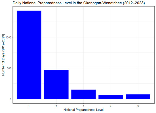
Figure A1.
Distribution of daily national preparedness level in the fall and spring (2012–2023).
Figure A1.
Distribution of daily national preparedness level in the fall and spring (2012–2023).


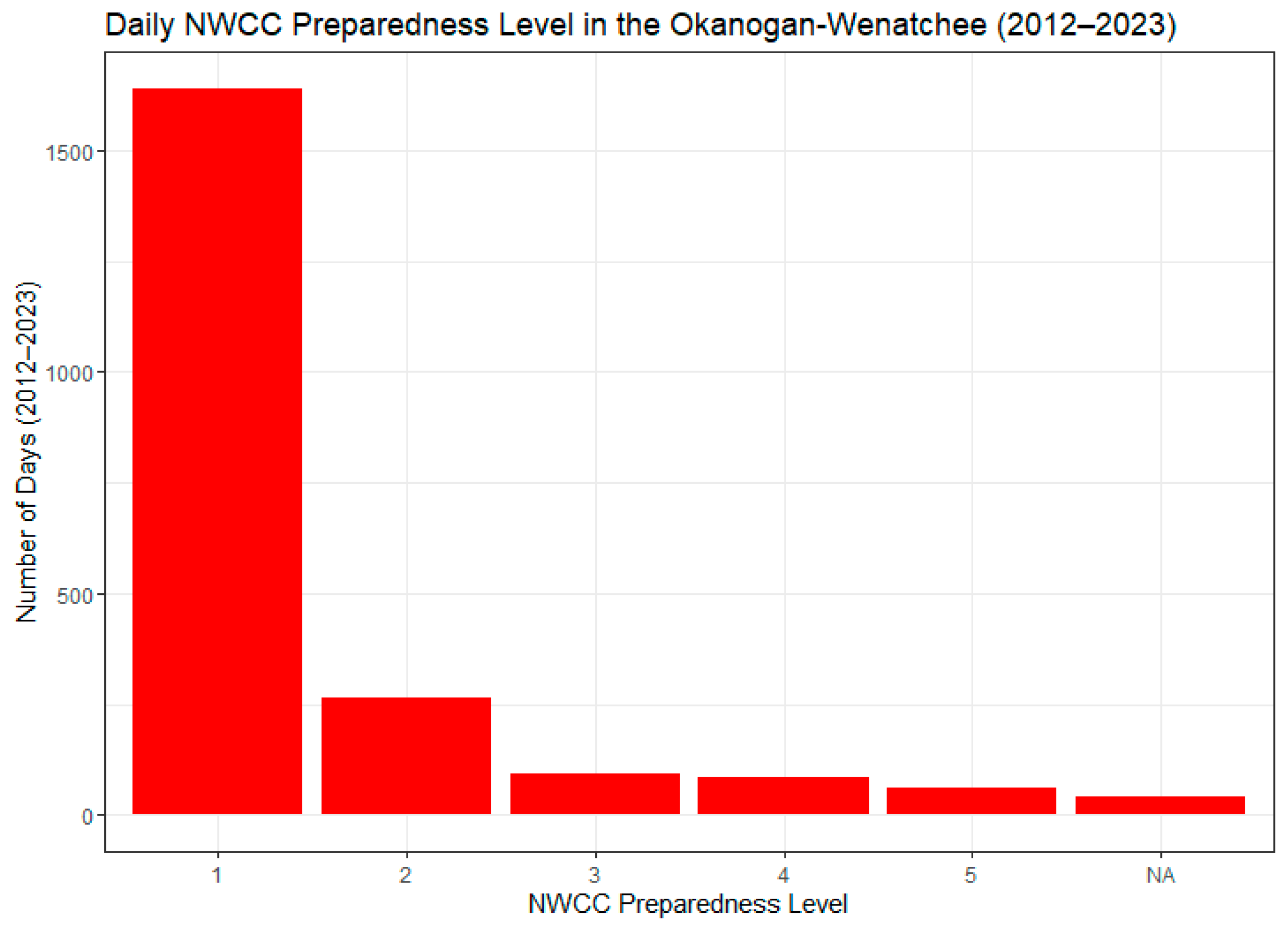
Figure A2.
Distribution of daily NWCC preparedness level in the fall and spring (2012–2023). GACC-level data was not available after 20 October 2023, so this does not include the end of October/November for 2023.
Figure A2.
Distribution of daily NWCC preparedness level in the fall and spring (2012–2023). GACC-level data was not available after 20 October 2023, so this does not include the end of October/November for 2023.
Appendix B
Additional PCA Analyses
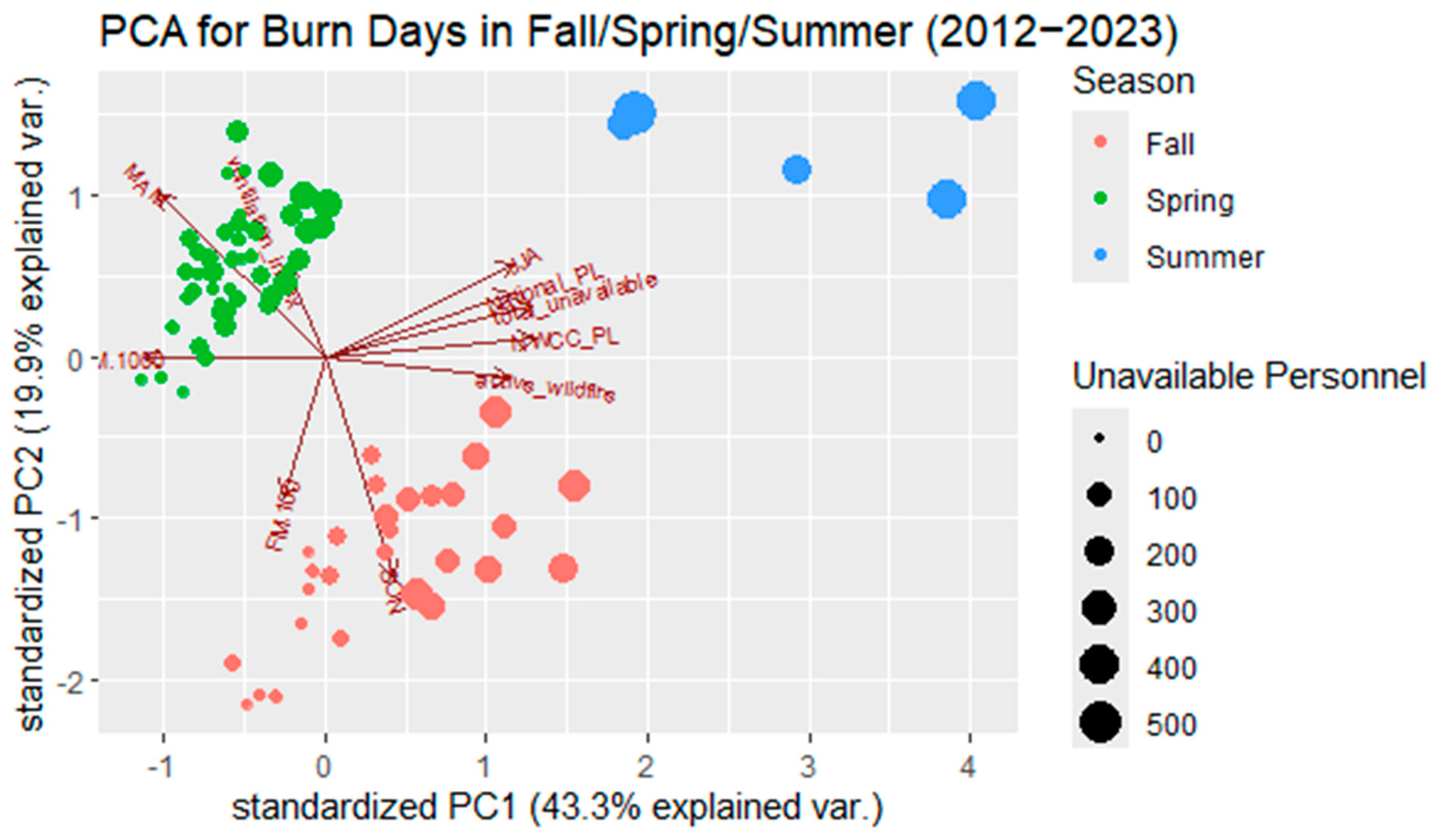
In addition to the principal component analysis (PCA) presented in the body of the paper, we conducted PCA on the following sets of days: (1) all days in fall, spring, and summer; (2) burn days in fall, spring, and summer; (3) all spring days; and (4) all fall days. Dates between 20 May 2022, and 18 August 2022, were excluded due to the pause on prescribed burning during this period.
We note that the summer burn days are distinct from fall and spring burn days, with higher PC1 and PC2 values (see Appendix B, Figure A4 below). There are very few summer burn days, and they are characterized differently than fall and spring burn days. This motivated our decision to focus the analysis in the body of the paper on fall and spring days.
- (1)
- All Days in Fall, Spring, and Summer
Table A3.
Principal component analysis for all days in fall, spring, and summer (2012–2023). Proportion of variance explained by each of the first four PCs, and loadings for each variable on each PC, are displayed.
Table A3.
Principal component analysis for all days in fall, spring, and summer (2012–2023). Proportion of variance explained by each of the first four PCs, and loadings for each variable on each PC, are displayed.
| PC1 | PC2 | PC3 | PC4 | |
| Proportion of Variance | 0.473 | 0.196 | 0.1 | 0.08 |
| Loadings | ||||
| PC1 | PC2 | PC3 | PC4 | |
| Total Personnel Unavailable | 0.37 | 0.035 | 0.023 | 0.078 |
| Acres of Active Wildfire (NWCC) | 0.268 | 0.335 | 0.545 | −0.044 |
| National PL | 0.419 | 0.078 | 0.187 | 0.029 |
| NWCC PL | 0.394 | 0.151 | 0.272 | 0.045 |
| FM100 | −0.333 | 0.283 | 0.069 | −0.16 |
| FM1000 | −0.399 | 0.085 | 0.117 | 0.006 |
| Ventilation Index | 0.086 | −0.383 | 0.159 | −0.902 |
| March/April/May | −0.279 | −0.331 | 0.593 | 0.218 |
| June/July/August | 0.323 | −0.313 | −0.393 | 0.088 |
| Sept/Oct/Nov | −0.039 | 0.645 | −0.208 | −0.307 |
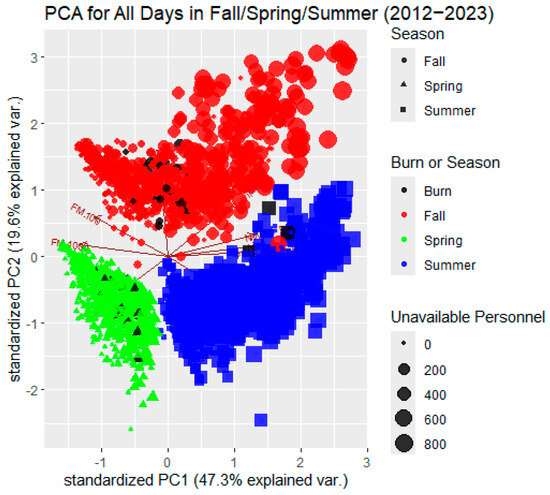
Figure A3.
Plot of PC2 vs. PC1 for all days in the fall, spring, and summer (2012–2023). Each marker represents one day. Fall days are represented by circular markers, spring days are represented by triangular markers, and summer days are represented by square markers. Green represents spring days on which no prescribed burn occurs, red represents fall days on which no prescribed burn occurs, blue represents summer days on which no prescribed burn occurs, and black represents prescribed burn days. Marker size indicates the number of unavailable personnel recorded for each day.

- (2)
- Burn Days in Fall, Spring, and Summer
Table A4.
Principal component analysis for burn days in fall, spring, and summer (2012–2023). Proportion of variance explained by each of the first four PCs, and loadings for each variable on each PC, are displayed.
Table A4.
Principal component analysis for burn days in fall, spring, and summer (2012–2023). Proportion of variance explained by each of the first four PCs, and loadings for each variable on each PC, are displayed.
| PC1 | PC2 | PC3 | PC4 | |
| Proportion of Variance | 0.433 | 0.199 | 0.124 | 0.087 |
| Loadings | ||||
| PC1 | PC2 | PC3 | PC4 | |
| Total Personnel Unavailable | 0.404 | 0.149 | −0.061 | 0.069 |
| Acres of Active Wildfire (NWCC) | 0.362 | −0.063 | −0.201 | 0.118 |
| National PL | 0.366 | 0.181 | −0.237 | 0.051 |
| NWCC PL | 0.414 | 0.053 | −0.093 | −0.035 |
| FM100 | −0.082 | −0.408 | −0.605 | 0.397 |
| FM1000 | −0.357 | −0.0002 | −0.527 | 0.099 |
| Ventilation Index | −0.077 | 0.257 | 0.344 | 0.89 |
| March/April/May | −0.324 | 0.473 | −0.15 | −0.097 |
| June/July/August | 0.371 | 0.269 | −0.194 | 0.054 |
| Sept/Oct/Nov | 0.135 | −0.64 | 0.262 | 0.071 |
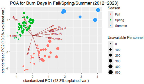
Figure A4.
Plot of PC2 vs. PC1 for burn days in the fall, spring, and summer (2012–2023). Each marker represents one day. Season is distinguished by color (fall by red marker, spring by green marker, and summer by blue marker). Marker size indicates the number of unavailable personnel recorded for each day.
- (3)
- All Spring Days
Table A5.
Principal component analysis for all days in spring (2012–2023). Proportion of variance explained by each of the first four PCs, and loadings for each variable on each PC, are displayed.
Table A5.
Principal component analysis for all days in spring (2012–2023). Proportion of variance explained by each of the first four PCs, and loadings for each variable on each PC, are displayed.
| PC1 | PC2 | PC3 | PC4 | |
| Proportion of Variance | 0.34 | 0.157 | 0.146 | 0.134 |
| Loadings | ||||
| PC1 | PC2 | PC3 | PC4 | |
| Total Personnel Unavailable | 0.454 | −0.143 | −0.151 | 0.206 |
| Acres of Active Wildfire (NWCC) | 0.216 | −0.314 | 0.456 | 0.296 |
| National PL | 0.431 | −0.439 | −0.152 | 0.112 |
| NWCC PL | 0.048 | 0.692 | −0.244 | 0.636 |
| FM100 | −0.507 | −0.303 | −0.149 | 0.363 |
| FM1000 | −0.543 | −0.279 | −0.189 | 0.18 |
| Ventilation Index | 0.084 | −0.202 | 0.793 | 0.538 |

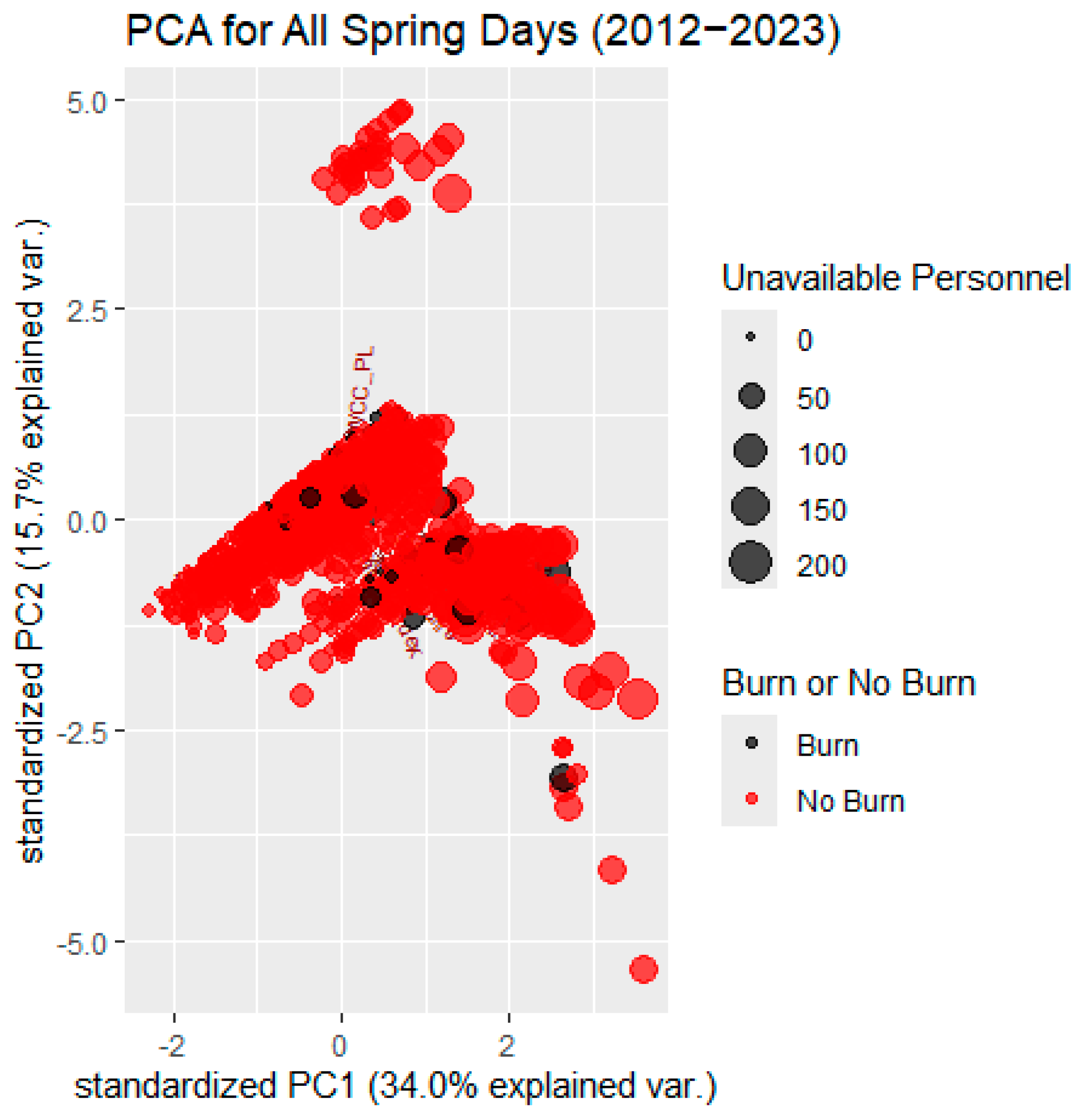
Figure A5.
Plot of PC2 vs. PC1 for all days in spring (2012–2023). Each marker represents one day. Burn status is distinguished by color (burn day by black markers and non-burn day by red markers). Marker size indicates the number of unavailable personnel recorded for each day.
Figure A5.
Plot of PC2 vs. PC1 for all days in spring (2012–2023). Each marker represents one day. Burn status is distinguished by color (burn day by black markers and non-burn day by red markers). Marker size indicates the number of unavailable personnel recorded for each day.
- (4)
- All Fall Days
Table A6.
Principal component analysis for all days in fall (2012–2023). Proportion of variance explained by each of the first four PCs, and loadings for each variable on each PC, are displayed.
Table A6.
Principal component analysis for all days in fall (2012–2023). Proportion of variance explained by each of the first four PCs, and loadings for each variable on each PC, are displayed.
| PC1 | PC2 | PC3 | PC4 | |
| Proportion of Variance | 0.613 | 0.153 | 0.117 | 0.047 |
| Loadings | ||||
| PC1 | PC2 | PC3 | PC4 | |
| Total Personnel Unavailable | −0.389 | 0.316 | 0.101 | −0.811 |
| Acres of Active Wildfire (NWCC) | −0.376 | 0.455 | 0.124 | 0.126 |
| National PL | −0.447 | 0.183 | 0.086 | 0.302 |
| NWCC PL | −0.446 | 0.075 | 0.003 | 0.441 |
| FM100 | 0.338 | 0.475 | 0.474 | 0.195 |
| FM1000 | 0.4 | 0.374 | 0.287 | −0.031 |
| Ventilation Index | −0.184 | −0.537 | 0.813 | −0.055 |
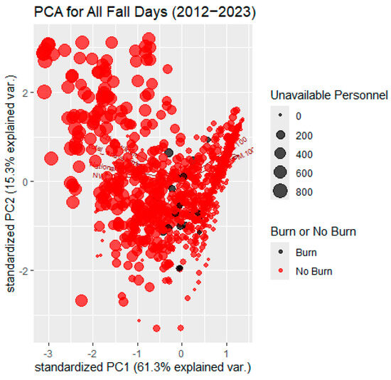
Figure A6.
Plot of PC2 vs. PC1 for all days in fall (2012–2023). Each marker represents one day. Burn status is distinguished by color (burn day by black markers and non-burn day by red markers). Marker size indicates the number of unavailable personnel recorded for each day.
Figure A6.
Plot of PC2 vs. PC1 for all days in fall (2012–2023). Each marker represents one day. Burn status is distinguished by color (burn day by black markers and non-burn day by red markers). Marker size indicates the number of unavailable personnel recorded for each day.

Appendix C
Analyses Using VIIRS Dates
As noted previously, the prescribed burn dates in the USFS FACTS database can be imprecise. Thus, we explore the possibility of a spatial merge of the FACTS data [16] with VIIRS (Visible Infrared Imaging Radiometer Suite) data [30], which uses a satellite to detect fires. We find that about a quarter of the prescribed burns are missing in the VIIRS data; thus, an absolute merge relying on matching all fires across the two datasets would omit many of the prescribed burns recorded in FACTS. Still, for the sake of comparison, we re-run the analyses substituting, where matched, the FACTS date with the date of the corresponding fire in VIIRS. For burns that have no counterpart in the VIIRS data, we retain the record with the date from FACTS. The analyses using this hybrid of VIIRS/FACTS are displayed below. We note that the PCA results and the logit results are substantially the same as those based on FACTS alone.
There is some imprecision in the dates entered in FACTS, which may introduce noise into the analysis; however, any attempt to correct for this also carries substantial risk for introducing new sources of error. Further, there is no reason to believe that the imprecision in FACTS is biasing the results. Finally, given the rate of missing fires in VIIRS (relative to FACTS) we cannot be confident that, where matches did occur, they represent the same incident in both datasets. Rather, it is possible that some of the matches are actually merging two separate events that occurred in close proximity spatially but on quite different dates. For these reasons, we retain a consistent approach by using the FACTS dataset in the main body of the paper while presenting a comparative analysis with a hybrid FACTS/VIIRS dataset here.
- Principal Component Analysis (PCA)
- 1.1
- Burn and Non-Burn Days (Spring/Fall)
Table A7.
Principal component analysis for all days in fall and spring (2012–2023). Proportion of variance explained by each of the first four PCs, and loadings for each variable on each PC, are displayed.
Table A7.
Principal component analysis for all days in fall and spring (2012–2023). Proportion of variance explained by each of the first four PCs, and loadings for each variable on each PC, are displayed.
| PC1 | PC2 | PC3 | PC4 | |
| Proportion of Variance | 0.522 | 0.182 | 0.116 | 0.079 |
| Loadings | ||||
| PC1 | PC2 | PC3 | PC4 | |
| Total Personnel Unavailable | 0.416 | −0.1 | −0.184 | 0.189 |
| Acres of Active Wildfire (NWCC) | 0.403 | −0.17 | −0.273 | 0.31 |
| National PL | 0.451 | −0.027 | −0.155 | 0.11 |
| NWCC PL | 0.449 | −0.05 | −0.085 | 0.013 |
| FM100 | −0.248 | −0.564 | −0.473 | −0.092 |
| FM1000 | −0.374 | −0.329 | −0.361 | 0.271 |
| Ventilation Index | 0.003 | 0.535 | −0.688 | −0.476 |
| Spring/Fall (Spring = 1) | −0.242 | 0.495 | −0.183 | 0.74 |

Figure A7.
Plot of PC2 vs. PC1 for all days in the fall and spring (2012–2023). Each marker represents one day. Fall days are represented by circular markers, while spring days are represented by triangular markers. Green represents spring days on which no prescribed burn occurs, red represents fall days on which no prescribed burn occurs, and black represents prescribed burn days. Marker size indicates the number of unavailable personnel recorded for each day. Burn dates are determined using VIIRS data, where possible.
1.2 Burn Days (Spring/Fall)
Table A8.
Principal component analysis for burn days in fall and spring (2012–2023). Proportion of variance explained by each of the first four PCs, and loadings for each variable on each PC, are displayed. Burn dates are determined using VIIRS data, where possible, in this parallel analysis.
Table A8.
Principal component analysis for burn days in fall and spring (2012–2023). Proportion of variance explained by each of the first four PCs, and loadings for each variable on each PC, are displayed. Burn dates are determined using VIIRS data, where possible, in this parallel analysis.
| PC1 | PC2 | PC3 | PC4 | |
| Proportion of Variance | 0.484 | 0.162 | 0.115 | 0.101 |
| Loadings | ||||
| PC1 | PC2 | PC3 | PC4 | |
| Total Personnel Unavailable | 0.439 | −0.085 | 0.263 | −0.281 |
| Acres of Active Wildfire (NWCC) | 0.355 | −0.351 | 0.03 | −0.401 |
| National PL | 0.353 | 0.088 | 0.341 | −0.388 |
| NWCC PL | 0.419 | −0.01 | −0.192 | 0.329 |
| FM100 | −0.142 | −0.705 | −0.417 | −0.22 |
| FM1000 | −0.445 | −0.206 | 0.085 | −0.28 |
| Ventilation Index | 0.055 | 0.526 | −0.674 | −0.507 |
| Spring/Fall (Spring = 1) | −0.4 | 0.213 | 0.375 | −0.343 |
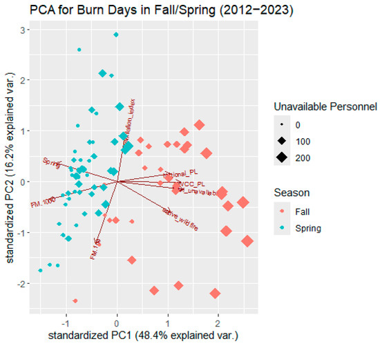
Figure A8.
Plot of PC2 vs. PC1 for burn days in the fall and spring (2012–2023). Each marker represents one day. Season is distinguished by color (fall by red markers, spring by blue markers). Marker size indicates the number of unavailable personnel recorded for each day. Burn dates are determined using VIIRS data, where possible, in this parallel analysis.
- 2.
- Logistic Regression Model
Table A9.
Logistic regression results for prescribed burning in the fall, spring, and fall/spring. Burn dates are determined using VIIRS data, where possible, in this parallel analysis.
Table A9.
Logistic regression results for prescribed burning in the fall, spring, and fall/spring. Burn dates are determined using VIIRS data, where possible, in this parallel analysis.
| Logit Model for Prescribed Burning in the Okanogan-Wenatchee (2012–2023) with VIIRS/FACTS | ||||||
|---|---|---|---|---|---|---|
| Dependent Variable: Prescribed Burn Day (Yes/No) | ||||||
| Fall β (s.e.) | Fall β (s.e.) | Spring β (s.e.) | Spring β (s.e.) | Fall/Spring β (s.e.) | Fall/Spring β (s.e.) | |
| (Intercept) | −1.2023 (0.7492) | −27.6495 *** (6.5399) | −0.7073 (0.8876) | −33.8075 *** (8.4069) | −1.0271 (0.5423) | −11.3336 *** (2.7688) |
| Total Personnel Unavailable | −0.0031 ** (0.0013) | −0.0038 ** (0.0015) | 0.0001 (0.0040) | 0.0015 (0.0042) | −0.0023 ** (0.0012) | −0.0013 (0.0012) |
| FM1000 | −0.1338 *** (0.0396) | 3.4258 *** (0.8673) | −0.0958 ** (0.0391) | 3.1962 *** (0.8455) | −0.1230 *** (0.0273) | 1.0808 *** (0.2948) |
| (FM1000)2 | - | −0.1146 *** (0.0286) | - | −0.0805 *** (0.0212) | - | −0.0321 *** (0.0079) |
| Ventilation Index | −0.0001 ** (0.00006) | −0.0002 * (0.00007) | −0.00008 * (0.00005) | −0.00005 (0.00004) | −0.00002 (0.00004) | −0.00001 (0.00004) |
| Spring/Fall (Spring = 1) | - | - | - | - | 0.7442 *** (0.2653) | −0.3498 (0.2604) |
| Observations | 1092 | 1092 | 1092 | 1092 | 2184 | 2184 |
| Akaike Inf. Crit. | 282.46 | 244.29 | 428.35 | 401.33 | 713.75 | 689.41 |
Note: * p < 0.1, ** p < 0.05, *** p < 0.01.
References
- Abatzoglou, J.T.; Williams, A.P. Impact of Anthropogenic Climate Change on Wildfire across Western US Forests. Proc. Natl. Acad. Sci. USA 2016, 113, 11770–11775. [Google Scholar] [CrossRef] [PubMed]
- Parks, S.A.; Abatzoglou, J.T. Warmer and Drier Fire Seasons Contribute to Increases in Area Burned at High Severity in Western US Forests From 1985 to 2017. Geophys. Res. Lett. 2020, 47, e2020GL089858. [Google Scholar] [CrossRef]
- Cullen, A.C.; Prichard, S.J.; Abatzoglou, J.T.; Dolk, A.; Kessenich, L.; Bloem, S.; Bukovsky, M.S.; Humphrey, R.; McGinnis, S.; Skinner, H.; et al. Growing Convergence Research: Coproducing Climate Projections to Inform Proactive Decisions for Managing Simultaneous Wildfire Risk. Risk Anal. 2023, 43, 2262–2279. [Google Scholar] [CrossRef]
- Prichard, S.J.; Hessburg, P.F.; Hagmann, R.K.; Povak, N.A.; Dobrowski, S.Z.; Hurteau, M.D.; Kane, V.R.; Keane, R.E.; Kobziar, L.N.; Kolden, C.A.; et al. Adapting Western North American Forests to Climate Change and Wildfires: 10 Common Questions. Ecol. Appl. 2021, 31, 1–30. [Google Scholar] [CrossRef]
- Quinn-Davidson, L.N.; Varner, J.M. Impediments to Prescribed Fire across Agency, Landscape and Manager: An Example from Northern California. Int. J. Wildland Fire 2012, 21, 210–218. [Google Scholar] [CrossRef]
- Kobziar, L.N.; Godwin, D.; Taylor, L.; Watts, A.C. Perspectives on Trends, Effectiveness, and Impediments to Prescribed Burning in the Southern U.S. Forests 2015, 6, 561–580. [Google Scholar] [CrossRef]
- Schultz, C.A.; McCaffrey, S.M.; Huber-Stearns, H.R. Policy Barriers and Opportunities for Prescribed Fire Application in the Western United States. Int. J. Wildland Fire 2019, 28, 874–884. [Google Scholar] [CrossRef]
- Miller, R.K.; Field, C.B.; Mach, K.J. Barriers and Enablers for Prescribed Burns for Wildfire Management in California. Nat. Sustain. 2020, 3, 101–109. [Google Scholar] [CrossRef]
- Smithwick, E.A.H.; Wu, H.; Spangler, K.; Adib, M.; Wang, R.; Dems, C.; Taylor, A.; Kaye, M.; Zipp, K.; Newman, P.; et al. Barriers and Opportunities for Implementing Prescribed Fire: Lessons from Managers in the Mid-Atlantic Region, United States. Fire Ecol. 2024, 20, 77. [Google Scholar] [CrossRef]
- Westerling, A.L. Increasing Western US Forest Wildfire Activity: Sensitivity to Changes in the Timing of Spring. Philos. Trans. R. Soc. Lond. Ser. B Biol. Sci. 2016, 371, 20150178. [Google Scholar] [CrossRef]
- Abatzoglou, J.T.; Battisti, D.S.; Williams, A.P.; Hansen, W.D.; Harvey, B.J.; Kolden, C.A. Projected Increases in Western US Forest Fire despite Growing Fuel Constraints. Commun. Earth Environ. 2021, 2, 227. [Google Scholar] [CrossRef]
- Hessburg, P.F.; Prichard, S.J.; Hagmann, R.K.; Povak, N.A.; Lake, F.K. Wildfire and Climate Change Adaptation of Western North American Forests: A Case for Intentional Management. Ecol. Appl. 2021, 31, e02432. [Google Scholar] [CrossRef] [PubMed]
- Harry, P.; Alison, C. Patterns and Trends in Simultaneous Wildfire Activity in the United States from 1984 to 2015. Int. J. Wildland Fire 2020, 29, 1057–1071. [Google Scholar] [CrossRef]
- Skinner, H.K.; Prichard, S.J.; Cullen, A.C. Decision Support for Landscapes with High Fire Hazard and Competing Values at Risk: The Upper Wenatchee Pilot Project. Fire 2024, 7, 77. [Google Scholar] [CrossRef]
- Gewers, F.L.; Ferreira, G.R.; De Arruda, H.F.; Silva, F.N.; Comin, C.H.; Amancio, D.R.; Costa, L.D.F. Principal Component Analysis: A Natural Approach to Data Exploration. ACM Comput. Surv. 2022, 54, 1–34. [Google Scholar] [CrossRef]
- Osborne, J.W. Best Practices in Logistic Regression; SAGE: Los Angeles, CA, USA, 2015. [Google Scholar]
- USFS. Hazardous Fuel Treatment Reduction—Polygon. 2024. Available online: https://data.fs.usda.gov/geodata/edw/datasets.php (accessed on 9 November 2024).
- Abatzoglou, J.T. Development of Gridded Surface Meteorological Data for Ecological Applications and Modelling. Int. J. Climatol. 2013, 33, 121–131. [Google Scholar] [CrossRef]
- ERA5. ECMWF Reanalysis v5. 2024. Available online: https://www.ecmwf.int/en/forecasts/dataset/ecmwf-reanalysis-v5 (accessed on 14 October 2024).
- Nguyen, D.; Belval, E.J.; Wei, Y.; Short, K.C.; Calkin, D.E. Dataset of United States Incident Management Situation Reports from 2007 to 2021. Sci. Data 2024, 11, 23. [Google Scholar] [CrossRef]
- Cullen, A.C.; Axe, T.; Podschwit, H. High-Severity Wildfire Potential—Associating Meteorology, Climate, Resource Demand and Wildfire Activity with Preparedness Levels. Int. J. Wildland Fire 2021, 30, 30–51. [Google Scholar] [CrossRef]
- IROC. Interagency Resource Ordering Capability. 2024. Available online: https://www.wildfire.gov/application/iroc (accessed on 4 November 2024).
- ROSS. Resource Ordering and Status System. Lockheed Martin Enterprise Solutions & Services. 2024. Available online: https://www.wildfire.gov/application/ross (accessed on 4 November 2024).
- Belval, E.J.; Stonesifer, C.S.; Calkin, D.E. Fire Suppression Resource Scarcity: Current Metrics and Future Performance Indicators. Forests 2020, 11, 217. [Google Scholar] [CrossRef]
- Washington State Department of Natural Resources (WA DNR). Join Our Seasonal Firefighting Team. Available online: https://www.dnr.wa.gov/wildfirejobs (accessed on 14 February 2025).
- Fossum, C.A.; Collins, B.M.; Stephens, C.W.; Lydersen, J.M.; Restaino, J.; Katuna, T.; Stephens, S.L. Trends in Prescribed Fire Weather Windows from 2000 to 2022 in California. For. Ecol. Manag. 2024, 562, 121966. [Google Scholar] [CrossRef]
- Knapp, E.E.; Estes, B.L.; Skinner, C.N. Ecological Effects of Prescribed Fire Season: A Literature Review and Synthesis for Managers. JFSP Synth. Rep. 2009, 4. Available online: http://digitalcommons.unl.edu/jfspsynthesis/4 (accessed on 7 April 2025).
- Podschwit, H.; Miller, C.; Alvarado, E. Spatiotemporal Prescribed Fire Patterns in Washington State, USA. Fire 2021, 4, 19. [Google Scholar] [CrossRef]
- Monsanto, P.G.; Agee, J.K. Long-Term Post-Wildfire Dynamics of Coarse Woody Debris After Salvage Logging and Implications for Soil Heating in Dry Forests of the Eastern Cascades, Washington. For. Ecol. Manag. 2008, 255, 3952–3961. [Google Scholar] [CrossRef]
- FIRMS. Fire Information for Research Management System. VIIRS S-NPP. 2025. Available online: https://firms.modaps.eosdis.nasa.gov/download/ (accessed on 22 February 2025).


Disclaimer/Publisher’s Note: The statements, opinions and data contained in all publications are solely those of the individual author(s) and contributor(s) and not of MDPI and/or the editor(s). MDPI and/or the editor(s) disclaim responsibility for any injury to people or property resulting from any ideas, methods, instructions or products referred to in the content. |
© 2025 by the authors. Licensee MDPI, Basel, Switzerland. This article is an open access article distributed under the terms and conditions of the Creative Commons Attribution (CC BY) license (https://creativecommons.org/licenses/by/4.0/).