Abstract
One of the primary challenges for future nuclear fusion power plants is understanding how neutron irradiation affects reactor materials. To tackle this issue, the IFMIF-DONES project aims to build a facility capable of generating a neutron source in order to irradiate different material samples. This will be achieved by colliding a deuteron beam with a lithium jet. In this work, within the DONES-FLUX project, deep learning surrogate models are applied to the design and optimization of the IFMIF-DONES linear accelerator. Specifically, neural operators are employed to predict deuteron beam envelopes along the longitudinal axis of the accelerator and neutron irradiation effects at the end, after the beam collision. This approach has resulted in models that are able of approximating complex simulations with high accuracy (less than 17% percentage error for the worst case) and significantly reduced inference time (ranging from 2 to 6 orders of magnitude) while being differentiable. The substantial speed-up factors enable the application of online reinforcement learning algorithms, and the differentiable nature of the models allows for seamless integration with differentiable programming techniques, facilitating the solving of inverse problems to find the optimal parameters for a given objective. Overall, these results demonstrate the synergy between deep learning models and differentiable programming, offering a promising collaboration among physicists and computer scientists to further improve the design and optimization of IFMIF-DONES and other accelerator facilities. This research will lay the foundations for future projects, where optimization efforts with differentiable programming will be performed.
1. Introduction
Nuclear fusion is a promising source of sustainable energy for humanity [1]. However, the design and validation of materials that can withstand the extreme conditions within a fusion reactor remains an open issue [2]. In order to replicate this environment, the IFMIF-DONES (International Fusion Materials Irradiation Facility-DEMO Oriented Neutron Source) project is developing a linear accelerator that will produce a neutron spectrum similar to that of nuclear fusion reactions by colliding deuterons with a flowing lithium target [3]. The resulting neutrons then irradiate material samples located in a high flux test module (HFTM), allowing for the study of its effects [4].
As part of the DONES-FLUX project, this research addresses the challenge of optimizing the IFMIF-DONES facility by employing differentiable deep learning surrogate models (DLSMs). Accurate simulations of this complex environment involve vast numbers of particles and an extensive parameter space, making them computationally intensive and time-consuming, sometimes taking days to complete [5]. This computational demand renders it unfeasible to apply optimization algorithms, such as gradient descent (GD) [6] or deep reinforcement learning (DRL) [7], which may require many iterations to converge. DLSMs provide an effective solution by approximating these simulations with a high accuracy while drastically reducing the inference time, thereby enabling the application of such optimization algorithms.
Neural operators (NOs) are a class of DLSM designed to approximate mappings between function spaces, making them highly effective for solving systems of partial differential equations (PDEs) that model complex physical phenomena [8]. Unlike traditional neural networks, which typically approximate finite-dimensional mappings, NOs work in infinite-dimensional spaces, which allows them to capture spatially continuous relationships between input functions and output functions [9]. For this study, the Fourier neural operator (FNO) [10] and deep operator network (DeepONet) [11] architectures were selected, which have the advantages of being purely data-driven and with a proven performance across a wide range of applications [12,13,14]. Additionally, FNO has the property of discretization invariance and can predict at different resolutions with the same trained model.
In this work, NO architectures are employed as DLSMs in two critical parts of the IFMIF-DONES neutron source. First, FNO models are trained to predict beam statistical functions and beam profile distributions in the initial section of the high energy beam transport line (HEBT-S1) line of the accelerator [15]. Second, a DeepONet architecture is used to model material irradiation variables within the HFTM [16] after the collision. The efficiency and differentiability of these models enable the optimization of the quadrupoles to achieve specific operational objectives in the facility. Section 2 details the materials and methodologies used, Section 3 presents the results for both applications, and Section 4 discusses the implications of these findings.
2. Materials and Methods
2.1. General Methodology
The general workflow involves the following steps: first, identify the specific part of the facility targeted for optimization. Next, perform simulations using traditional solvers to generate a representative dataset. Then, train the differentiable DLSMs using this dataset. Finally, integrate the trained models into other applications that require speed and differentiability. This process is visually summarized in Figure 1.
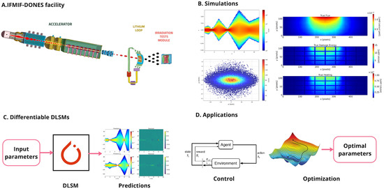
Figure 1.
Optmization processworkflow. (A) Select the facility part and frame the problem. (Image credit: IFMIF-DONES) (B) Generate dataset with traditional simulations. (C) Train differentiable DLSMs with the data. (D) Employ the models for different applications.
2.2. Optimizing the HEBT-S1 Lattice
The first problem is to determine the optimal values for the magnets in the HEBT-S1 section, which is illustrated in the left side of Figure 2. The lattice comprises six quadrupoles (from now on represented by the integer j) and their corresponding drift spaces. The lengths, apertures, and field strengths of each component are defined as in [17] and are detailed in Table A4 of Appendix A. A set of coordinates is employed, where represent the transversal axes and z describes the accelerator longitude. This lattice configuration was implemented in the OPAL simulator [18].
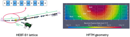
Figure 2.
(Left):The IFMIF-DONES HEBT, with the S1 components, quadrupoles, and drift zones. Taken from [15]. (Right): Two-dimensional slices of the geometry of the HFTM. Taken from [16].
A total number of 8192 deuteron beam simulations were conducted, each with a different set of magnetic field values , spanning the 4–8 range. The simulation outputs included the one-dimensional statistical beam functions and (Root mean square (RMS) and maximum size of the envelopes (MAX)) and the normalized number of particles . The two-dimensional beam profile distributions, and , were also recorded. Each simulation corresponded to a single deuteron bunch crossing the lattice, with 100,000 injected particles generated from Gaussian distributions (see Table A1 of Appendix A for the injection parameters).
From the entire dataset of simulations, 20% was reserved for testing, while the remaining 80% was used for training the models. Two different models were developed: a 1D-FNO to predict the statistical beam functions and particle counts, and a 2D-FNO to predict the beam profile distributions. A summary of the models is presented in Equation (1) and the full architectures with their hyperparameters are detailed in Table A6 of Appendix C. NVIDIA Modulus, version 1.5.0 [19] and PyTorch 2.3.0 [20] were selected as frameworks because of the FNO implementation and differentiable computational graph capability.
Finally, the 1D model was combined with a GD optimization algorithm, Adam [21], to explore the parameter space and solve the inverse problem of determining the optimal quadrupole settings needed to achieve the desired beam configurations at the end of the lattice (related to the beam footprint, the RMS, MAX, and n functions evaluated at m). This method is effective because the trained models are differentiable with respect to the input parameters, . Details of the optimizer and other algorithm hyperparameters are provided in Table A7 of Appendix C, whereas the loss function is described in Equation (A1) of Appendix E. The different terms in the loss function minimize the discrepancy between the objective and current beam configurations and impose penalties on out-of-bound solutions. A summary of the software and hardware resources used in this work is presented in Table A5 of Appendix B.
2.3. Surrogates for Materials Irradiation Variables in HFTM
As previously mentioned, the accelerated deuteron beam interacts with liquid lithium, initiating the Li(d, xn) stripping reaction [22], which generates high-energy neutrons to replicate the radiation conditions of a nuclear fusion reactor. In order to evaluate the mechanical properties of the materials intended for these reactors, the samples were placed inside the HFTM, shown on the right side of Figure 2, where they were exposed to varying degrees of neutron flux to cover different irradiation quantities. Preliminary studies on the variables influenced by radiation must be conducted through simulations. In IFMIF-DONES, Monte Carlo (MC) codes deliver the most accurate results, albeit at a significant computational cost. This is due to the statistical nature of the method, which requires a large number of source particles to achieve statistically reliable solutions, resulting in prolonged computational times [23].
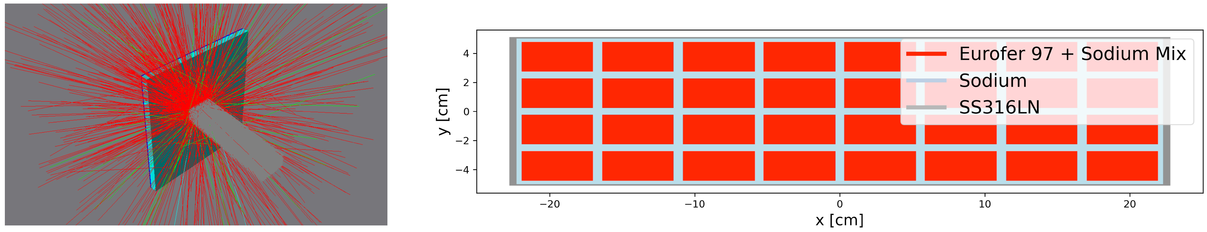
To simulate that process and gather the necessary data for training the model, a coupling between Geant4 [24] and OpenMC [25] was established, as illustrated in Figure 3. First, Geant4 models the Li(d, xn) stripping reaction, where deuterium and lithium interact to generate high-energy neutrons (>14 MeV). This is achieved by simulating a deuteron beam interacting with a 25 mm lithium curtain, positioned in front of a detector. The detector captures key data, including the position, angle, and energy of particles from the reaction, particularly the neutrons. Next, the collected data serve as the input for the second simulator, OpenMC, which simulates neutron transport in HFTM and calculates magnitudes such as flux, damage energy, heating, and hydrogen and helium production. Figure 4 illustrates the Geant4 and OpenMC simulations. On the left, a simple representation of the lithium curtain and the deuteron beam is shown, while the right side of the figure depicts a vertical cross-section of the HFTM model. The simulation process is repeated with varying parameters (see ranges in Table 1). This simulation setup is a simplification of the IFMIF-DONES setup, as the main purpose of this study is to validate the data-driven model. For a high resolution physical model, refer to [26]. Future works will integrate more precise physical representations of the system.
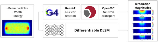
Figure 3.
Neutronic DLSM process. Using the spatial and energy distribution of the deuteron beam, a Geant4 simulation is conducted to determine the neutron flux. This flux data are then input into the OpenMC to model the variables influencing the materials within the HFTM.

Figure 4.
(Left): Lithium curtain and deuteron beam in Geant4. The red tracks correspond to neutrons, while the green tracks to photons. (Right): Vertical section of the HFTM modelled in OpenMC.

Table 1.
Input parameter ranges for the deuteron beam. See Table A2 for details on the simulation arguments.
The OpenMC simulator has been validated for the IFMIF-DONES facility in other works [27] where the McDeLicious extension [22] for the Li(d, xn) stripping reaction for MCNP has been adapted [28]. However, this extension is not Open Source, and for reproducibility purposes, the alternative use of Geant4 has been choosen, acknowledging the decriment in the generation of reliable physics data. See Table A3 for a summary of the OpenMC tallies used in this work.
The NO model utilized for this task is based on the DeepONet architecture [11], implemented using the DeepXDE library [29]. This architecture comprises two distinct sub-networks: the branch network and the trunk network. The input data are divided, such that neutron source parameters are processed by the branch, while spatial coordinates are managed by the trunk. This operation and the result of merging both nets to produce an output as an operator G can be seen in Equation (2).
Five separate models are trained, each corresponding to a specific variable (flux, damage energy, heating, hydrogen production, and helium production). To evaluate improvements in inference time, each model is trained with 100 training samples, 25 validation samples, and 25 test samples (only 150 simulations were utilized due to the significant computational resources needed to calculate the neutronic tallies. In contrast, the deuteron models required a substantially larger number of simulations to accurately capture the beam dynamics behavior).
3. Results
3.1. Quadrupoles Optimization in the HEBT-S1 Lattice
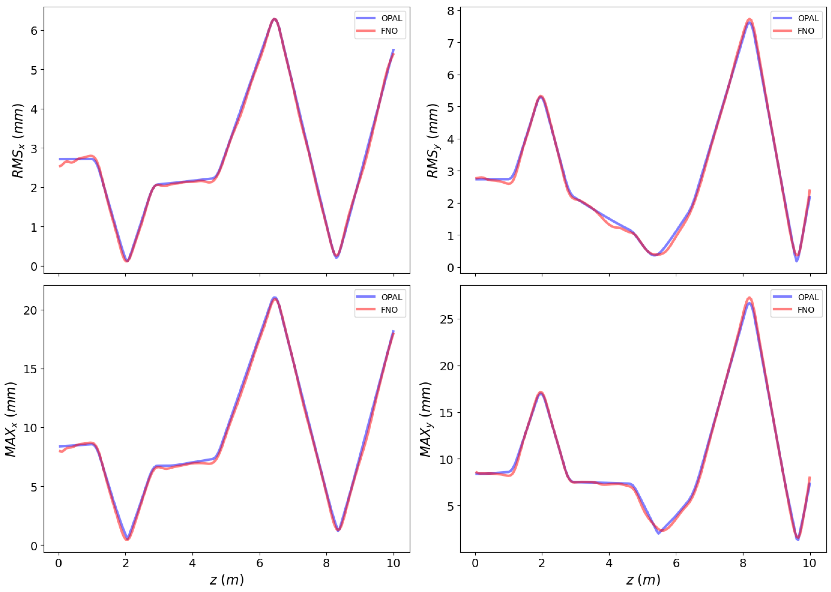
The 1D-FNO model is able to predict all of the beam statistical functions and the number of particles times faster than the OPAL code, with a trade-off mean average percentage error (MAPE) of 3.60% across all variables (see Table A10 of Appendix F for the individual errors). Figure 5 displays a test example of the results obtained by the model, compared with the simulations. Some instances for the predicted number of particles are also shown in Figure A3 of Appendix G.
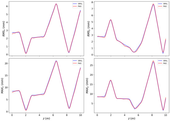
Figure 5.
Prediction results for the 1D beam statistics functions along the accelerator’s longitudinal axis, shown for the x and y axes. Blue lines represent OPAL simulations, while red lines indicate FNO predictions.
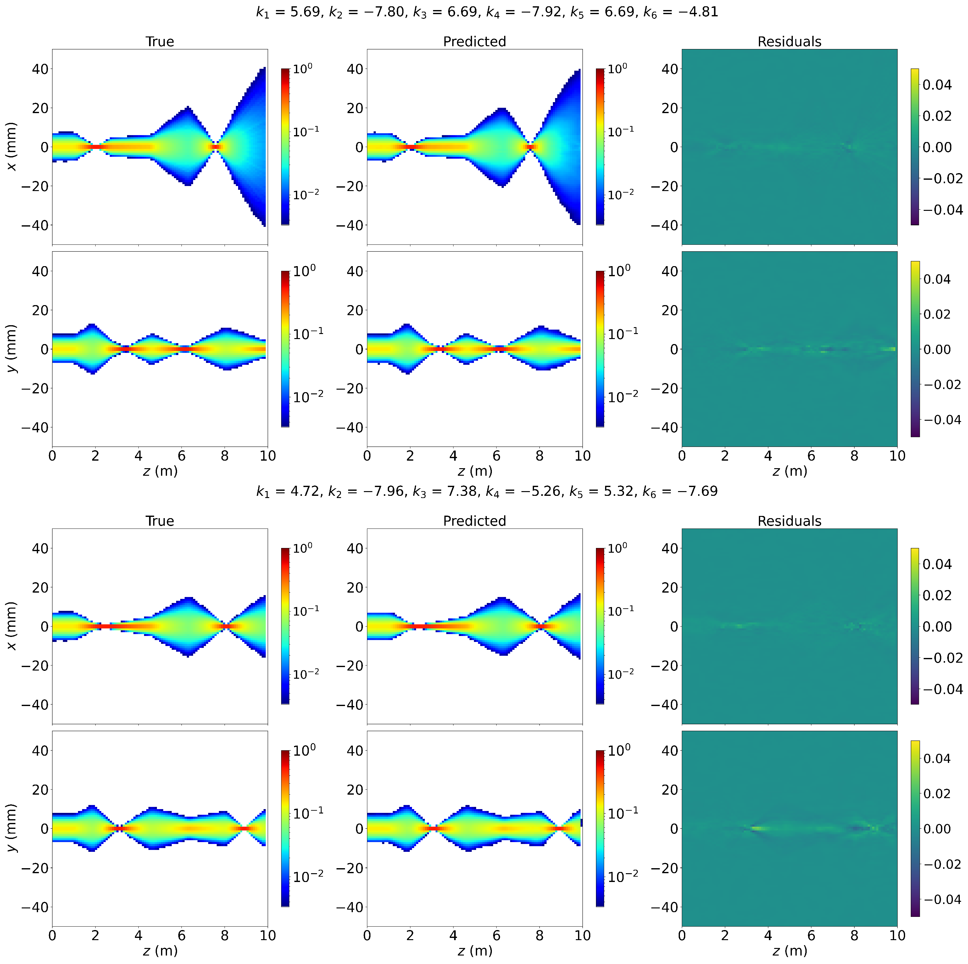
Figure 6 presents the predictions of the beam profile distributions model for a test example, alongside the corresponding OPAL simulations and residual errors. The model achieves a mean absolute error (MAE) of 5.15 on the test set. The inference speed boost factor matches that of the previous model, as both rely on the same set of simulations. A comprehensive summary of error metrics for each function across both models is provided in Table A10 of Appendix F, with additional test examples of the model predictions also available in Figure A5 of Appendix G.
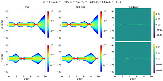
Figure 6.
Test prediction results for the 2D beam profile distributions along the accelerator’s longitudinal axis, displayed for the x and y axes. The (left) panel shows OPAL simulations, the (middle) panel presents FNO predictions, and the (right) panel illustrates the residual errors.
Table A9 of Appendix D summarizes the optimization outcomes for different beam objectives, presenting the target and achieved configurations for the statistical beam functions evaluated at m. The table also details the optimized quadrupole values, the computational time required to converge to a solution, and the particle count as reported by OPAL during the evaluation. A consistent threshold of was applied as a loss optimization criterion, ensuring the particle losses remained below 2%. The optimization process reliably achieved the desired objectives within approximately 10 min.
3.2. Neutronic Irradiation Models for HFTM
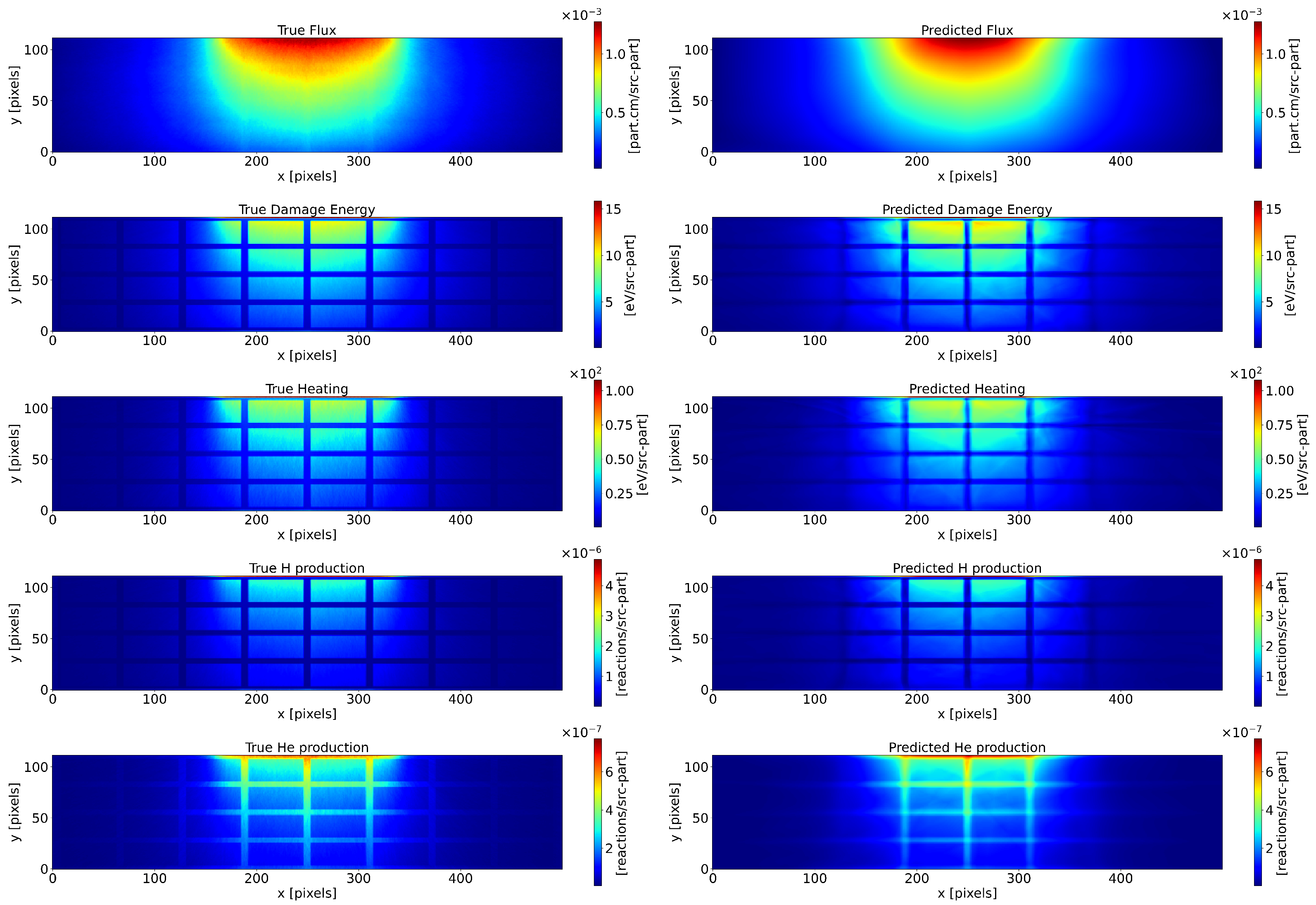
The prediction results are shown in Figure 7 and its corresponding errors in Figure 8. Using 100 training samples, DeepONet successfully learns the geometry of the HFTM and delivers accurate predictions. The 150 instances of the dataset took a total of s to generate, resulting in an average time per simulation of s. The inference time of DeepONet per simulation was s, resulting in a speedup factor of . The performance metrics achieved by DeepONet are summarized in Table A11, in Appendix F. Finally, the numerical simulation results used to train these models were not validated and should not be referenced in future works.
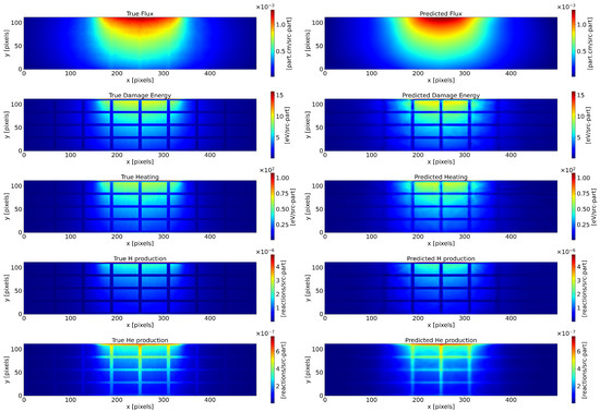
Figure 7.
Neutronic variables predictions. (Left): Geant4 and OpenMC coupled output. (Right): The DeepONet prediction. For each predicted variable, a different model produces the output.
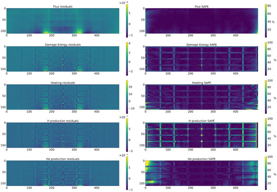
Figure 8.
Errors in the neutronic predictions. (Left): Residuals for each magnitude. (Right): Symmetric Absolute Percentage Error (SAPE) for every magnitude. This metric has the visible limitation where it sets to 100% when a 0 true value is encountered.
4. Discussion
In this study, NO operator models were trained as differentiable DLSMs to significantly enhance the inference speed of traditional simulations. These properties enable their use in optimization loops and applications that would otherwise require an impractical number of time steps. The developed models significantly reduced the inference times, with factors ranging from to , while maintaining minimal error metrics. However, it is important to note that these models create predictions at unseen points within the trained input space and, thus, do not extrapolate. This would require architectures like Physics-Informed Neural Operators (PINOs) [30], which integrate physical constraints for improved generalization. Additionally, the deuteron beam optimization procedure manages to reach all of the established objectives mantaining particle counts and ensuring the desired footprint geometry, which is a key factor for the collision.
These results not only demonstrate the potential of DLSMs for optimization tasks, but their applications extend beyond solving inverse problems. As shown in other studies, including [31], the significant reduction in simulation time enables the online training of deep reinforcement learning agents for control and tuning. These algorithms often require millions of time steps to converge and the efficiency of surrogate models makes this feasible.
While the results are promising, there are certain limitations that are being currently addressed. The optimization was restricted to the HEBT-S1 section due to the exponential growth in computational resources required as the number of magnetic elements increased. Further works will include new sampling strategies more suited to high-dimensional spaces of parameters and other optimization strategies. Furthermore, incorporating additional channels into the models, such as particle momentum data, could enhance optimization by providing phase-space information, a critical factor in particle accelerator operations [32]. This refinement has the potential to improve the model performance and to broaden their applicability. Future works will address this with the inclusion of quality beam outputs, like emmitance, in model predictions, and including these features in the objective optimization function to find not only the parameters that provide an objective shape, but also the ones that have the best beam quality.
The limitations of the current DeepOnet model for neutrionics predictions are that if the geometry changes, a new re-training has to be created. To address this issue, future works will include the use of novel geometry-aware models, like Geom-DeepOnet [33], with a generalization capability for different geometries. Addionally, the HFTM model will be updated with the final IFMIF-DONES version for a more precise representation.
In conclusion, the trained NO models represent a significant step forward in beam dynamics simulation and neutron irradiation. By leveraging their speed, accuracy, and differentiability, they offer compelling solutions for the challenges faced in the IFMIF-DONES neutron source and other scientific facilities.
Author Contributions
Conceptualization, R.G.-E.M., G.R.-L., G.G.R., L.M.R. and R.M.N.; methodology, G.G.R., G.R.-L., L.M.R. and R.M.N.; software, G.G.R., G.R.-L., L.M.R. and R.M.N.; validation, G.G.R., G.R.-L., L.M.R., N.K.P. and R.M.N.; formal analysis, G.G.R., G.R.-L., L.M.R. and R.M.N.; investigation, G.G.R., G.R.-L., L.M.R. and R.M.N.; resources, R.G.-E.M.; data curation, G.G.R., G.R.-L. and L.M.R.; writing—original draft preparation, G.G.R., G.R.-L., L.M.R. and N.K.P.; writing—review and editing, R.G.-E.M. and R.L.O.; visualization, G.G.R., G.R.-L., L.M.R., N.K.P. and R.M.N.; supervision, R.G.-E.M. and G.R.-L.; project administration, R.G.-E.M. and G.R.-L.; funding acquisition, R.G.-E.M. All authors have read and agreed to the published version of the manuscript.
Funding
The project DONES-FLUX, with file number MIP-20221017, has been subsidised by the CDTI—Centro de Desarrollo Tecnológico Industrial through the call for proposals of the “Misiones CDTI” programme for the year 2022 and it is supported by the Ministry of Science and Innovation of Spain.
Data Availability Statement
The data presented in this study are available upon reasonable request from the corresponding author due to restrictions imposed by the proprietary information guidelines established by the Spanish Centre for the Development, Technology and Innovation (CDTI).
Acknowledgments
We wish to acknowledge and thank the other participants of DONES-FLUX project, the IFMIF-DONES consortium as well as the University of Granada for their role played in the development of this work.
Conflicts of Interest
The authors declare no conflicts of interest.
Abbreviations
The following abbreviations are used in this manuscript:
| DLSM | Deep Learning Surrogate Model |
| DeepONet | Deep Operator Network |
| DRL | Deep Reinforcement Learning |
| FFT | Fast Fourier Transform |
| FNO | Fourier Neural Operator |
| GD | Gradient Descent |
| HEBT-S1 | 1st section of the High Energy Beam Transport line |
| HFTM | High Flux Test Module |
| IFMIF-DONES | International Fusion Materials Irradiation Facility-Demo Oriented Neutron Source |
| MAE | Mean Absolute Error |
| MAPE | Mean Average Percentage Error |
| MC | Monte Carlo |
| MSE | Mean Square Error |
| NMAE | Normalized Mean Average Error |
| NO | Neural Operator |
| PDE | Partial differential equations |
| RMS | Root Mean Square |
| sMAPE | Symmetric Mean Average Percentage Error |
Appendix A. Physical Parameters for the Simulations
Table A1.
Summary of the key parameters for the OPAL-T configuration used in the simulation. Data employed in this work should be fully reproducible using the set-up displayed in this Section.
Table A1.
Summary of the key parameters for the OPAL-T configuration used in the simulation. Data employed in this work should be fully reproducible using the set-up displayed in this Section.
| Variable | Value | Description |
|---|---|---|
| Particle | Deuteron | Type of particle used for simulation. |
| Number of particles | 100,000 | Number of particles in the simulation. |
| Energy | 40 MeV | Energy of the particles in the simulation. |
| Injection type | Gauss | Type of distribution used for the injection |
| 28 mm | Standard deviations for the spatial distribution in x, y, and z. | |
| 0.023 | Standard deviations for the momentum distribution in x and y. | |
| 0.039 | Standard deviation for the momentum distribution in z. | |
| MAXSTEPS | 10,000 | Maximum number of simulation steps. |
| DT | 1.65 | Time step for the simulation. |
| ZSTOP | 10 | Stop condition for the z-coordinate during the simulation. |
| METHOD | PARALLEL-T | The OPAL mode. |
| FIELDSOLVER | FFT | Field solver method used in the simulation. |
| 16 | Number of grid points in the x, y, and t directions. | |
| PARFFTX,Y,T | true | Whether the FFT solver is parallelized for x, y, and t. |
| BCFFTX,Y,T | open | Boundary conditions used for the FFT solver in x, y, and t. |
| BBOXINCR | 1 | Increment for the bounding box size. |
| GREENSF | STANDARD | Green’s function type used in the simulation. |
Table A2.
Summary of the key parameters for the OpenMC and Geant4 configurations used in the simulation. Data employed in this work should be fully reproducible using the set-up displayed in this Section.
Table A2.
Summary of the key parameters for the OpenMC and Geant4 configurations used in the simulation. Data employed in this work should be fully reproducible using the set-up displayed in this Section.
| Variable | Value | Description |
|---|---|---|
| OpenMC | ||
| Run mode | Fixed source | Simulation mode with a constant neutron source. |
| Cross-section library | FENDL 3.2 | Cross-section library used in the simulation. |
| Boundary type | Vacuum | Boundary condition to simulate no reflection at the walls. |
| Material package | neutronics_material_maker | Python library to import materials such as Eurofer 97. |
| Geant4 | ||
| PhysicsList | QGSP_BIC_AllHP | Physics list for accurate modeling of Li(d,xn) stripping reactions. |
Table A3.
Summary of the tally setup used in the OpenMC simulation.
Table A3.
Summary of the tally setup used in the OpenMC simulation.
| Variable | Description |
|---|---|
| Tally Scores | |
| Flux | Tracks the total particle flux. |
| Heating (MT = 301) | Nuclear heating associated with the reaction rates. |
| Damage-energy (MT = 444) | Calculates the damage energy produced by the reactions. |
| H Production (n, p) | Tally for hydrogen (H) production via (n, p) reactions. |
| He Production (n, a) | Tally for helium (He) production through (n, ) reactions. |
| Filters | |
| MeshFilter | Covers the entire volume of the HFTM geometry. |
Table A4.
Magnetic element dimensions, length, and edge where it starts relative to the beginning of the lattice. The aperture radius of all the elements is r = 50 mm. This setup is displayed in Figure 2.
Table A4.
Magnetic element dimensions, length, and edge where it starts relative to the beginning of the lattice. The aperture radius of all the elements is r = 50 mm. This setup is displayed in Figure 2.
| Element | Length (m) | Edge (m) | Element Type |
|---|---|---|---|
| DR1 | 1.00 | 0.00 | Drift |
| Q1 | 0.25 | 1.00 | Quadrupole |
| DR2 | 0.60 | 1.25 | Drift |
| Q2 | 0.25 | 1.85 | Quadrupole |
| DR3 | 0.60 | 2.10 | Drift |
| Q3 | 0.25 | 2.70 | Quadrupole |
| DR4 | 1.65 | 2.95 | Drift |
| Q4F | 0.25 | 4.60 | Quadrupole |
| DR5 | 1.50 | 4.85 | Drift |
| Q5 | 0.25 | 6.35 | Quadrupole |
| DR6 | 1.50 | 6.60 | Drift |
| Q6 | 0.25 | 8.10 | Quadrupole |
| DR7 | 1.65 | 8.35 | Drift |
Appendix B. System Specifications
Table A5.
System and software specifications.
Table A5.
System and software specifications.
| Category | Specification |
|---|---|
| System Specifications | |
| GPU Model | NVIDIA GeForce RTX 3060 |
| CUDA Version | 12.2 |
| CPU Model | Intel(R) Core(TM) i9-10900K @ 3.70 GHz |
| CPUs | 12 |
| Software Specifications | |
| OS | Ubuntu 22.04.4 LTS (Docker) |
| nvidia-modulus.sym | 1.5.0 |
| OPAL | 2022.1.0 |
| openmpi | 4.1.4 |
| Torch | 2.3.0 |
| Geant4 | 11.2.1 |
| OpenMC | 0.14.0 |
| DeepXDE | 1.12.0 |
Appendix C. Hyperparameters
Table A6.
Hyperparameters for the FNO architectures in NVIDIA Modulus are shared between models when a single value is specified. For parameters with two values, the first corresponds to the 1D model, and the second to the 2D model.
Table A6.
Hyperparameters for the FNO architectures in NVIDIA Modulus are shared between models when a single value is specified. For parameters with two values, the first corresponds to the 1D model, and the second to the 2D model.
| Hyperparameter | Value |
|---|---|
| scheduler | tf_exponential_lr |
| optimizer | adam |
| loss | sum |
| decoder.nr_layers | 1 |
| decoder.layer_size | 256–512 |
| fno.dimension | 1–2 |
| fno.nr_fno_layers | 4 |
| fno.fno_modes | 12 |
| scheduler.decay_rate | 0.95 |
| scheduler.decay_steps | 1000 |
| training.max_steps | 10,000 |
| batch_size.grid | 32–8 |
| batch_size.validation | 32–8 |
Table A7.
Gradient descent optimization hyperparameters.
Table A7.
Gradient descent optimization hyperparameters.
| Hyperparameter | Value |
|---|---|
| scheduler | exponential_lr |
| optimizer | adam |
| loss | custom distance |
| scheduler.gamma | 0.999 |
| max_steps | 100,000 |
| early_stop_loss | 0.005 |
| learning_rate | 1 |
Table A8.
DeepONet hyperparameters.
Table A8.
DeepONet hyperparameters.
| Hyperparameter | Value |
|---|---|
| # trainable parameters | |
| Input layers (Trunk) | 2 neurons |
| Input layers (Branch) | 3 neurons |
| Hidden layers (Trunk) | 6 layers of 100 neurons |
| Hidden layers (Branch) | 5 layers of 50 neurons + 1 of 100 neurons |
| Output layer | 1 neuron |
| Training epochs | |
| Batch size | 1 full image ( points) |
| Learning rate and decay rate | and |
| Optimizer | Adam |
| Loss | MSE |
| Regularization | L2 regularization with L2 parameter |
Appendix D. Optimization Results
Table A9.
Optimization examples of beam configurations chosen to showcase different geometric shapes. The algorithm is capable of finding solutions as long as they are within the feasible solution space. All of the functions are evaluated at the footprint location, m.
Table A9.
Optimization examples of beam configurations chosen to showcase different geometric shapes. The algorithm is capable of finding solutions as long as they are within the feasible solution space. All of the functions are evaluated at the footprint location, m.
| Target (mm) | Achieved (mm) | (Tm−1) | t (min) | n | |||||||||||
|---|---|---|---|---|---|---|---|---|---|---|---|---|---|---|---|
| RMSx | RMSy | MAXx | MAXy | RMSx | RMSy | MAXx | MAXy | k1 | k2 | k3 | k4 | k5 | k6 | ||
| 5.4 | 2.4 | 18.0 | 8.0 | 5.4 | 2.4 | 17.9 | 8.0 | 5.9 | −7.1 | 6.9 | −5.2 | 5.0 | −6.3 | 10.42 | 1.00 |
| 4.7 | 2.6 | 16.0 | 7.0 | 4.7 | 2.6 | 15.6 | 6.9 | 5.1 | −5.7 | 7.6 | −6.4 | 5.1 | −6.0 | 3.42 | 0.99 |
| 2.5 | 3.4 | 9.0 | 12.0 | 2.6 | 3.1 | 8.9 | 12.0 | 5.0 | −8.0 | 7.4 | −7.7 | 5.0 | −6.9 | 10.44 | 1.00 |
| 3.0 | 3.0 | 11.0 | 10.0 | 3.0 | 3.0 | 10.5 | 9.8 | 5.3 | −6.7 | 7.9 | −8.0 | 5.0 | −6.0 | 1.52 | 0.99 |
| 6.4 | 8.5 | 22.0 | 30.0 | 6.3 | 8.5 | 21.5 | 27.0 | 5.4 | −6.2 | 7.9 | −6.3 | 5.4 | −7.2 | 3.34 | 0.99 |
| 11.8 | 10.4 | 38.9 | 33.0 | 11.7 | 10.3 | 39.0 | 32.5 | 5.0 | −6.3 | 7.9 | −6.6 | 5.9 | −7.5 | 10.45 | 0.99 |
| 16.5 | 1.0 | 50.0 | 3.4 | 16.5 | 1.0 | 49.8 | 3.3 | 6.5 | −7.5 | 7.1 | −5.6 | 6.5 | −5.8 | 2.30 | 0.99 |
| 9.8 | 10.2 | 33.4 | 37.3 | 9.8 | 10.2 | 32.5 | 31.3 | 5.0 | −6.0 | 7.6 | −6.3 | 5.6 | −7.4 | 3.7 | 0.99 |
| 7.0 | 6.6 | 23.5 | 19.5 | 7.0 | 6.0 | 23.2 | 19.5 | 6.4 | −7.8 | 6.2 | −5.0 | 5.0 | −7.8 | 10.43 | 0.99 |
| 13.3 | 4.3 | 48.6 | 14.2 | 13.3 | 4.3 | 45.7 | 13.6 | 5.5 | −6.5 | 7.7 | −6.5 | 6.2 | −6.4 | 1.48 | 0.99 |
| 7.7 | 11.6 | 25.9 | 29.9 | 7.7 | 11.6 | 25.9 | 29.4 | 6.0 | −5.0 | 5.1 | −6.0 | 5.0 | −7.3 | 4.31 | 0.98 |
| 4.2 | 13.1 | 14.5 | 37.5 | 4.1 | 13.1 | 14.5 | 36.7 | 5.0 | −5.5 | 5.0 | −6.9 | 5.0 | −7.6 | 10.47 | 0.99 |
It is important to note that for the optimization problem set in the Section 2.2 there can be multiple solutions that achieve the shape and particle loss goals.
Appendix E. Loss Function for the Optimization Algorithm
The optimization loss function is formulated as the Euclidean distance between the RMSi target configuration (denoted as T, from target) and the current configuration. Additionally, penalty terms are incorporated to discourage solutions that violate predefined bounds. These penalties are calculated for the quadrupole settings, the MAXi variables, and the particle count n, ensuring compliance with established thresholds. The components of the loss function are detailed as follows:
In this equation, x represents variables such as , MAXi, and n. The parameters l and u denote the respective lower and upper bounds for these variables. Specifically, the quadrupole ranges are constrained between 4 and 8 Tm−1, the MAXi values are bounded between 0 and their respective target values, and n is limited to the range of 0.98 to 1. The penalty weights w are set at 10 for the MAX variables and 100 for both the quadrupole settings and n. Here, i refers to the x and y coordinates, while j corresponds to the index of the quadrupoles.
Appendix F. Errors
Table A10.
FNO model errors evaluated in all the test set. The first part shows the 1D model errors, and the second part shows the 2D model errors. No MAPE is displayed for the 2D model due to the very small values of the pixels.
Table A10.
FNO model errors evaluated in all the test set. The first part shows the 1D model errors, and the second part shows the 2D model errors. No MAPE is displayed for the 2D model due to the very small values of the pixels.
| FNO 1D Model Errors | ||
| Variable | MAPE (%) | MAE |
| RMSx | 4.38 | 0.11 |
| RMSy | 5.63 | 0.16 |
| MAXx | 3.92 | 0.30 |
| MAXy | 3.76 | 0.39 |
| 0.92 | 0.01 | |
| FNO 2D Model Errors | ||
| Variable | MAPE (%) | MAE |
| - | 4.7 | |
| - | 5.6 | |
Table A11.
Mean sMAPE, NMAE, and R2 of the DeepONet model.
Table A11.
Mean sMAPE, NMAE, and R2 of the DeepONet model.
| Variable | sMAPE (%) | NMAE | R2 |
|---|---|---|---|
| Flux | 2.3 | 0.031 | 0.996 |
| Damage E. | 9.2 | 0.120 | 0.968 |
| Heating | 8.9 | 0.111 | 0.972 |
| H prod. | 16.8 | 0.139 | 0.967 |
| He prod. | 8.3 | 0.095 | 0.977 |
Appendix G. More Test Examples
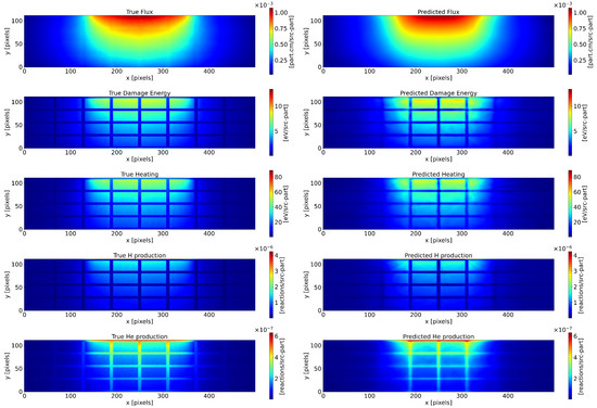
Figure A1.
Test sample of the DeepONet predictions.
Figure A1.
Test sample of the DeepONet predictions.
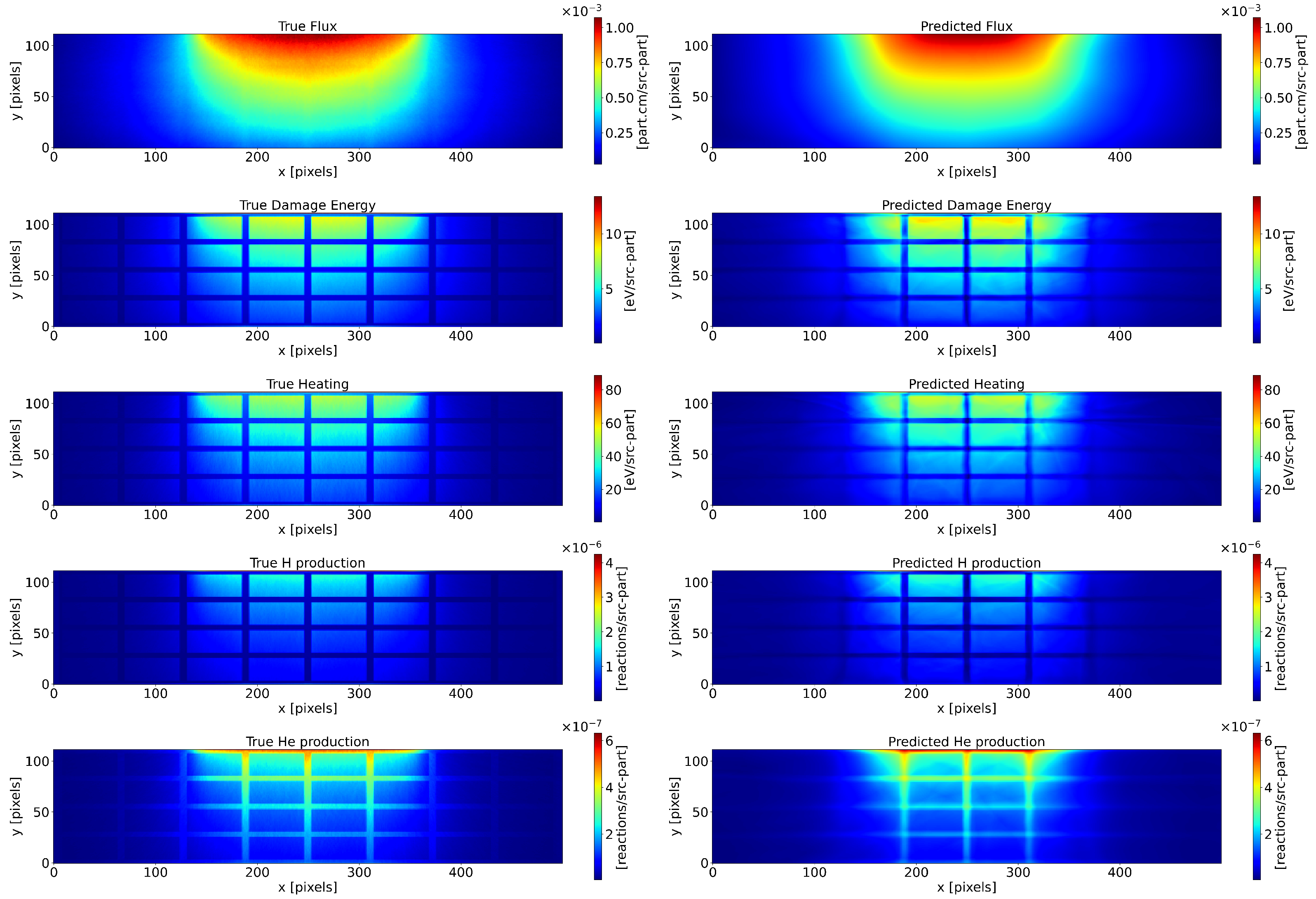
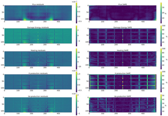
Figure A2.
Errors of the test sample above. (Left): Residuals for each magnitude. (Right): Symmetric absolute percentage error (SAPE) for every magnitude. This metric has the visible limitation where it sets to 100% when a 0 true value is encountered.
Figure A2.
Errors of the test sample above. (Left): Residuals for each magnitude. (Right): Symmetric absolute percentage error (SAPE) for every magnitude. This metric has the visible limitation where it sets to 100% when a 0 true value is encountered.
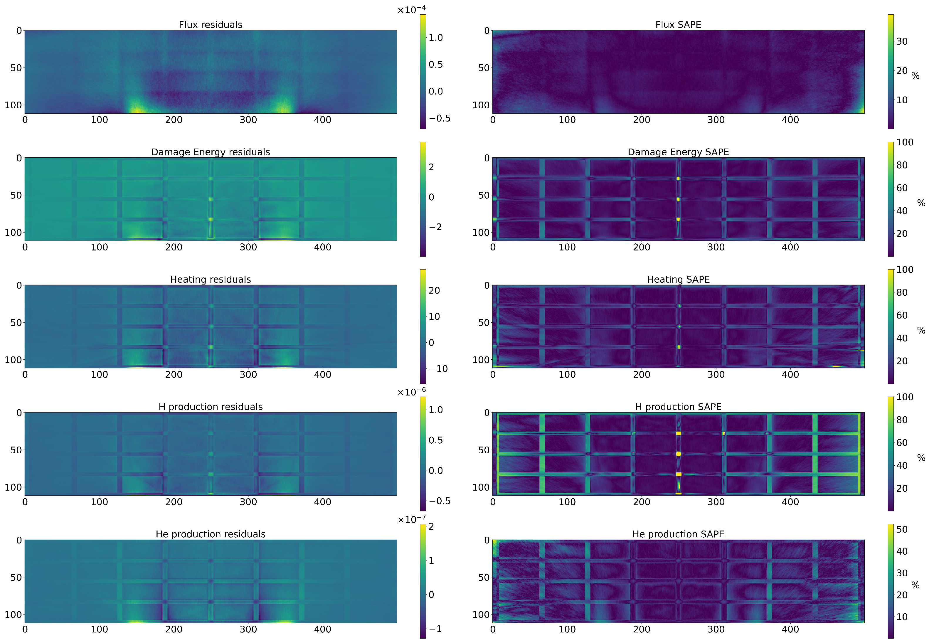
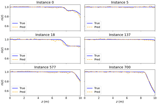
Figure A3.
Test instances of some predicted number of particles compared to the OPAL simulations.
Figure A3.
Test instances of some predicted number of particles compared to the OPAL simulations.
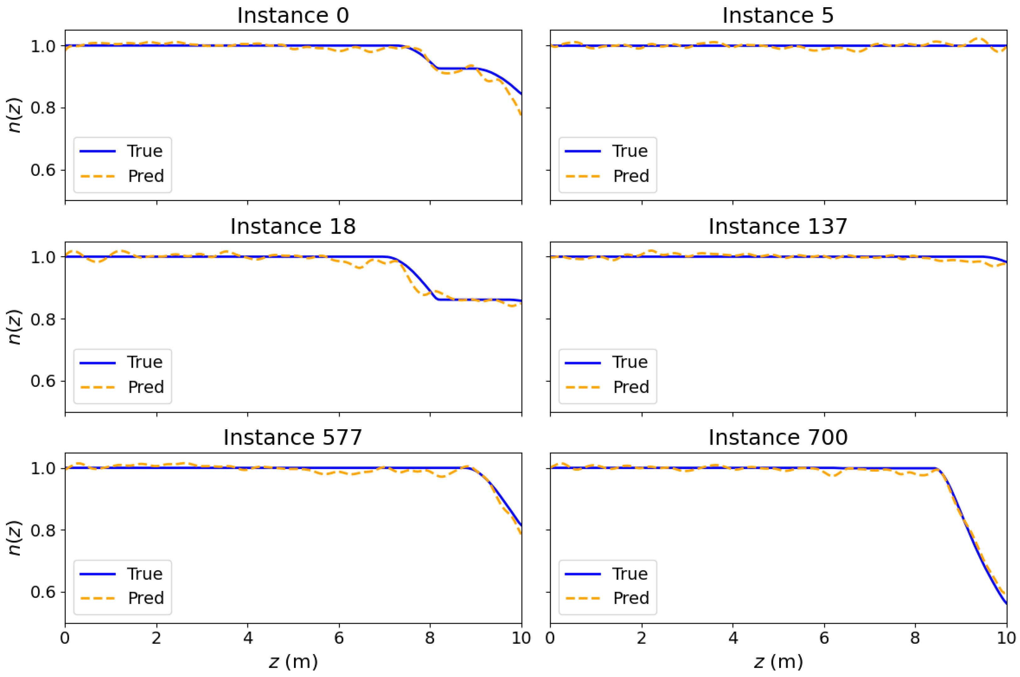
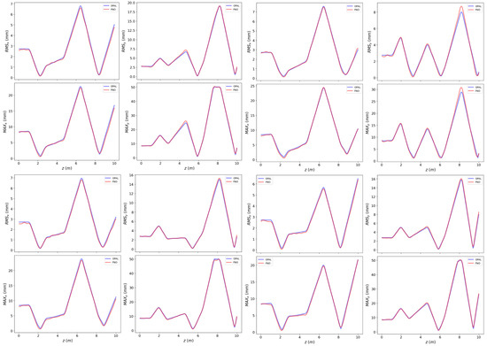
Figure A4.
More test instances of the predicted beam statistics compared to the OPAL simulations.
Figure A4.
More test instances of the predicted beam statistics compared to the OPAL simulations.
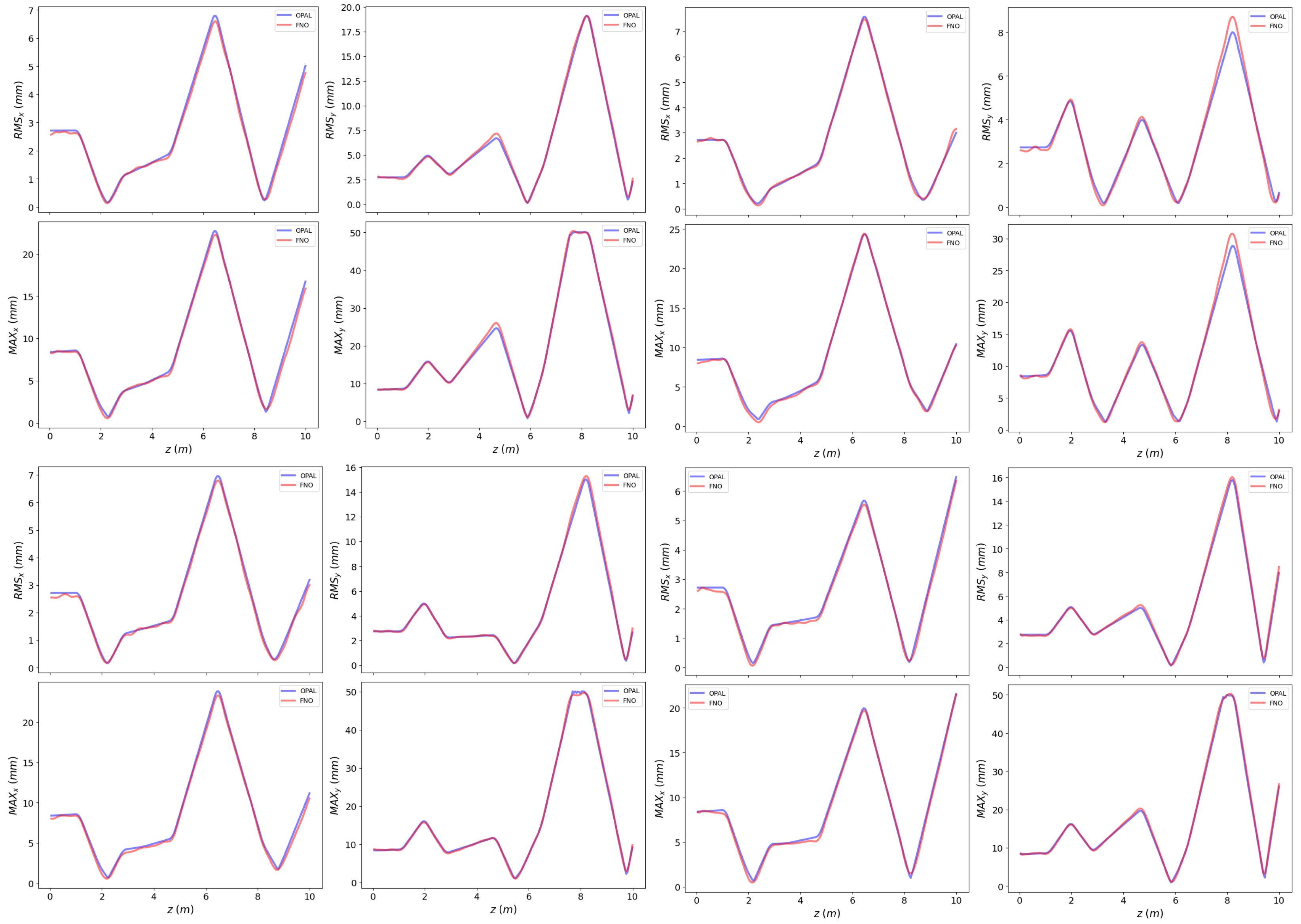
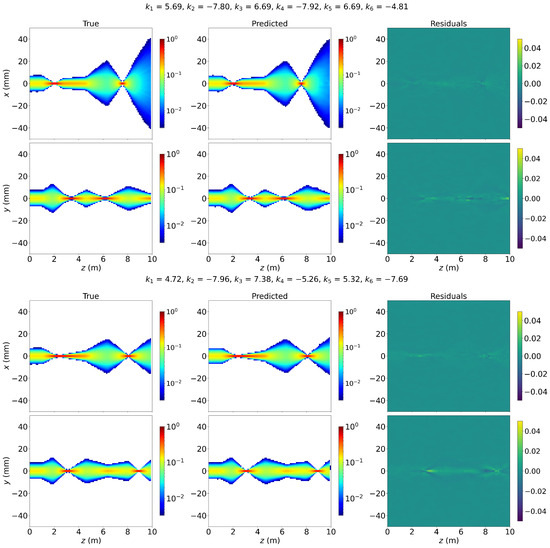
Figure A5.
More test instances of the predicted beam profiles compared to the OPAL simulations.
Figure A5.
More test instances of the predicted beam profiles compared to the OPAL simulations.
References
- Sadik-Zada, E.R.; Gatto, A.; Weißnicht, Y. Back to the Future: Revisiting the Perspectives on Nuclear Fusion and Juxtaposition to Existing Energy Sources. Energy 2024, 290, 129150. [Google Scholar] [CrossRef]
- Alba, R.; Iglesias, R.; Cerdeira, M.Á. Materials to Be Used in Future Magnetic Confinement Fusion Reactors: A Review. Materials 2022, 15, 6591. [Google Scholar] [CrossRef]
- Ibarra, A.; Arbeiter, F.; Bernardi, D.; Krolas, W.; Cappelli, M.; Fischer, U.; Heidinger, R.; Martin-Fuertes, F.; Micciché, G.; Muñoz, A.; et al. The European Approach to the Fusion-like Neutron Source: The IFMIF-DONES Project. Nucl. Fusion 2019, 59, 065002. [Google Scholar] [CrossRef]
- Qiu, Y.; Arbeiter, F.; Fischer, U.; Schwab, F. IFMIF-DONES HFTM Neutronics Modeling and Nuclear Response Analyses. Nucl. Mater. Energy 2018, 15, 185–189. [Google Scholar] [CrossRef]
- Zhu, Y.; Zabaras, N.; Koutsourelakis, P.S.; Perdikaris, P. Physics-Constrained Deep Learning for High-Dimensional Surrogate Modeling and Uncertainty Quantification without Labeled Data. J. Comput. Phys. 2019, 394, 56–81. [Google Scholar] [CrossRef]
- Ruder, S. An Overview of Gradient Descent Optimization Algorithms. arXiv 2017, arXiv:1609.04747. [Google Scholar]
- Li, Y. Deep Reinforcement Learning: An Overview. arXiv 2017, arXiv:1701.07274. [Google Scholar]
- Azizzadenesheli, K.; Kovachki, N.; Li, Z.; Liu-Schiaffini, M.; Kossaifi, J.; Anandkumar, A. Neural Operators for Accelerating Scientific Simulations and Design. Nat. Rev. Phys. 2024, 6, 320–328. [Google Scholar] [CrossRef]
- Kovachki, N.; Li, Z.; Liu, B.; Azizzadenesheli, K.; Bhattacharya, K.; Stuart, A.; Anandkumar, A. Neural Operator: Learning Maps between Function Spaces with Applications to PDEs. J. Mach. Learn. Res. 2024, 24, 4061–4157. [Google Scholar]
- Li, Z.; Kovachki, N.; Azizzadenesheli, K.; Liu, B.; Bhattacharya, K.; Stuart, A.; Anandkumar, A. Fourier Neural Operator for Parametric Partial Differential Equations. arXiv 2021, arXiv:2010.08895. [Google Scholar]
- Lu, L.; Jin, P.; Karniadakis, G.E. DeepONet: Learning Nonlinear Operators for Identifying Differential Equations Based on the Universal Approximation Theorem of Operators. Nat. Mach. Intell. 2021, 3, 218–229. [Google Scholar] [CrossRef]
- Pathak, J.; Subramanian, S.; Harrington, P.; Raja, S.; Chattopadhyay, A.; Mardani, M.; Kurth, T.; Hall, D.; Li, Z.; Azizzadenesheli, K.; et al. FourCastNet: A Global Data-driven High-resolution Weather Model Using Adaptive Fourier Neural Operators. arXiv 2022, arXiv:2202.11214. [Google Scholar]
- Kushwaha, S.; Park, J.; Koric, S.; He, J.; Jasiuk, I.; Abueidda, D. Advanced Deep Operator Networks to Predict Multiphysics Solution Fields in Materials Processing and Additive Manufacturing. arXiv 2024, arXiv:2403.14795. [Google Scholar] [CrossRef]
- Kobayashi, K.; Alam, S.B. Deep Neural Operator-Driven Real-Time Inference to Enable Digital Twin Solutions for Nuclear Energy Systems. Sci. Rep. 2024, 14, 2101. [Google Scholar] [CrossRef]
- Podadera, I.; Ibarra, A.; Jiménez-Rey, D.; Mollá, J.; Nomen, O.; Oliver, C.; Sánchez-Herranz, D.; Varela, R.; Villamayor, V. Beam Diagnostics for the Multi-MW High Energy Beam Transport Line of DONES. In Proceedings of the 8th International Beam Instrumentation Conference (IBIC’19), Malmö, Sweden, 8–12 September 2019; JACOW Publishing: Geneva, Switzerland, 2019; pp. 200–204. [Google Scholar] [CrossRef]
- Álvarez, I.; Anguiano, M.; Mota, F.; Hernández, R.; Qiu, Y. Neutronic Assessment of the IFMIF-DONES HFTM Specimen Stack Distribution. Fusion Eng. Des. 2024, 200, 114212. [Google Scholar] [CrossRef]
- Oliver, C.; Dzitko, H.; Ibarra, A.; Mollá, J.; Nomen, O.; Podadera, I.; Sánchez-Herranz, D.; Varela, R. Impact of the Magnet Alignment and Field Errors on the Output Uniform Beam at the DONES HEBT Line. In Proceedings of the 12th International Particle Accelerator Conference 2021, IPAC2021, Campinas, Brazil, 24–28 May 2021; pp. 3251–3253. [Google Scholar] [CrossRef]
- Adelmann, A.; Calvo, P.; Frey, M.; Gsell, A.; Locans, U.; Metzger-Kraus, C.; Neveu, N.; Rogers, C.; Russell, S.; Sheehy, S.; et al. OPAL a Versatile Tool for Charged Particle Accelerator Simulations. arXiv 2019, arXiv:1905.06654. [Google Scholar]
- Hennigh, O.; Narasimhan, S.; Nabian, M.A.; Subramaniam, A.; Tangsali, K.; Rietmann, M.; Ferrandis, J.d.A.; Byeon, W.; Fang, Z.; Choudhry, S. NVIDIA SimNetTM: An AI-accelerated Multi-Physics Simulation Framework. arXiv 2020, arXiv:2012.07938. [Google Scholar]
- Paszke, A.; Gross, S.; Massa, F.; Lerer, A.; Bradbury, J.; Chanan, G.; Killeen, T.; Lin, Z.; Gimelshein, N.; Antiga, L.; et al. PyTorch: An Imperative Style, High-Performance Deep Learning Library. arXiv 2019, arXiv:1912.01703. [Google Scholar]
- Kingma, D.P.; Ba, J. Adam: A Method for Stochastic Optimization. arXiv 2017, arXiv:1412.6980. [Google Scholar]
- Simakov, S.P.; Fischer, U.; Kondo, K.; Pereslavtsev, P. Status of the McDeLicious Approach for the D-Li Neutron Source Term Modeling in IFMIF Neutronics Calculations. Fusion Sci. Technol. 2012, 62, 233–239. [Google Scholar] [CrossRef]
- Serikov, A.; FISCHER, U.; GROSSE, D. High Performance Parallel Monte Carlo Transport Computations for ITER Fusion Neutronics Applications. Prog. Nucl. Sci. Technol. 2011, 2, 294–300. [Google Scholar] [CrossRef]
- Agostinelli, S.; Allison, J.; Amako, K.; Apostolakis, J.; Araujo, H.; Arce, P.; Asai, M.; Axen, D.; Banerjee, S.; Barrand, G.; et al. Geant4—A Simulation Toolkit. Nucl. Instruments Methods Phys. Res. Sect. A Accel. Spectrometers Detect. Assoc. Equip. 2003, 506, 250–303. [Google Scholar] [CrossRef]
- Romano, P.K.; Horelik, N.E.; Herman, B.R.; Nelson, A.G.; Forget, B.; Smith, K. OpenMC: A State-of-the-Art Monte Carlo Code for Research and Development. Ann. Nucl. Energy 2015, 82, 90–97. [Google Scholar] [CrossRef]
- Álvarez, I.; Anguiano, M.; Mota, F.; Hernández, R.; Moro, F.; Noce, S.; Qiu, Y.; Park, J.; Arbeiter, F.; Palermo, I.; et al. Comparative Analysis of Neutronic Features for Various Specimen Payload Configurations within the IFMIF-DONES HFTM. Fusion Eng. Des. 2025, 210, 114729. [Google Scholar] [CrossRef]
- Hu, Y.; Qiu, Y.; Fischer, U.; Lu, Y. Benchmarking and Verification of the OpenMC Code for Accelerator-Based Neutron Source Analyses. Fusion Eng. Des. 2021, 170, 112512. [Google Scholar] [CrossRef]
- Mendoza, E.; Cano-Ott, D.; Ibarra, A.; Mota, F.; Podadera, I.; Qiu, Y.; Simakov, S.P. Nuclear Data Libraries for IFMIF-DONES Neutronic Calculations. Nucl. Fusion 2022, 62, 106026. [Google Scholar] [CrossRef]
- Lu, L.; Meng, X.; Mao, Z.; Karniadakis, G.E. DeepXDE: A Deep Learning Library for Solving Differential Equations. SIAM Rev. 2021, 63, 208–228. [Google Scholar] [CrossRef]
- Li, Z.; Zheng, H.; Kovachki, N.; Jin, D.; Chen, H.; Liu, B.; Azizzadenesheli, K.; Anandkumar, A. Physics-Informed Neural Operator for Learning Partial Differential Equations. arXiv 2023, arXiv:2111.03794. [Google Scholar] [CrossRef]
- Rodríguez-Llorente, G.; Romero, G.G.; Martín, R.G.E. Applications of Fourier Neural Operators in the Ifmif-Dones Accelerator. In Proceedings of the ICLR 2024 Workshop on AI4DifferentialEquations in Science, Vienna, Austria, 7–11 May 2024. [Google Scholar]
- Lindstrøm, C.A.; Thévenet, M. Emittance Preservation in Advanced Accelerators. J. Instrum. 2022, 17, P05016. [Google Scholar] [CrossRef]
- He, J.; Koric, S.; Abueidda, D.; Najafi, A.; Jasiuk, I. Geom-DeepONet: A Point-Cloud-Based Deep Operator Network for Field Predictions on 3D Parameterized Geometries. Comput. Methods Appl. Mech. Eng. 2024, 429, 117130. [Google Scholar] [CrossRef]


Disclaimer/Publisher’s Note: The statements, opinions and data contained in all publications are solely those of the individual author(s) and contributor(s) and not of MDPI and/or the editor(s). MDPI and/or the editor(s) disclaim responsibility for any injury to people or property resulting from any ideas, methods, instructions or products referred to in the content. |
© 2025 by the authors. Licensee MDPI, Basel, Switzerland. This article is an open access article distributed under the terms and conditions of the Creative Commons Attribution (CC BY) license (https://creativecommons.org/licenses/by/4.0/).