A Binary Integer Programming Method for Optimal Wind Turbines Allocation

Abstract

The present study introduces a Binary Integer Programming (BIP) method to minimize the number of wind turbines needed to be installed in a wind farm. The locations of wind turbines are selected in a virtual grid which is constructed considering a minimum distance between the wind turbines to avoid the wake effect. Additional equality constraints are also included to the proposed formulation to prohibit or enforce the installation of wind turbines placement at specific locations of the wind farmland. Moreover, a microscopic wind turbine placement considering the local air density is studied. To verify the efficiency of this proposal, a square site was subdivided into 25 square cells providing a virtual grid with 36 candidate placement locations. Moreover, a virtual grid with 121 vertices related with a Greek island is also tested. All simulations conducted considering the area of geographical territory, the length of wind turbine blades, as well as the capacity of each turbine.

1. Introduction

The modern power grids are complex networks involving a range of energy sources. Traditionally, the production of electric energy took place in the so-called conventional power stations where fossil fuels were used. More recently, the nuclear stations were used in order to increase the amount of produced power energy [1]. However, in the last decade, there was a tendency to adopt renewable energy sources, like wind, sun, and biomass, which are characterized by limited environmental impact. These plants are gradually acquiring significance in many areas and countries. Of all these renewable sources, wind presents the highest penetration and is the most favorable renewable generation option.

Wind turbine generates electricity by making use of renewable wind energy, capturing the wind’s kinetic energy and transforming it into electric power. A wind turbine array installed at a distinct geographical area, producing a desired amount of power, is called a wind farm [2]. If the values of the total power required from the wind farm and the capacity of each wind turbine are known, we can determine the maximum number of wind turbines needed to be installed in a specific area. The amount of power generated in a wind farm is dependent on various conditions, such as the morphology of the land, the direction and speed of the wind, and the dimension and characteristics of turbines.

In the last years, the optimal wind turbines allocation problem, known also as the wind farm location optimization problem (WFLO), has been introduced in the literature and several methods have been proposed to solve it [3,4,5,6,7,8,9,10,11,12]. In [3], the optimal locations of wind turbines are calculated using a genetic search code in conjunction with wake superposition. Considering horizontal-axis wind turbines, the 3-D methodology presented in [4] determines their interference effects and performance as well as their flow-field. The interface, enhancement and evaluation of wake and boundary layer models were the main targets examined by the Efficient Development of Offshore Windfarms (ENDOW) project introduced in [5]. The genetic algorithm used in [6] provides the optimal solution of the problem ensuring the minimum number of wind turbines selected and limiting the wind farm territory occupied. In works [7,8,9], the wind turbine placement has been optimally addressed using a simulated annealing algorithm, a genetic algorithm, and a greedy algorithm, respectively. In [10], Monte Carlo simulations are used to optimally arrange the wind turbines in a wind farm. Real-coded genetic algorithms are adopted to solve the optimal placement of wind turbines in [11], while a particle swarm optimization model is introduced for the optimal micro-placement of wind farms in [12]. In [13], the problem is solved considering three cost components of wind turbines dependent on the machine, the tower height, and the generator location. A comprehensive study of WFLO considering both cost and maintenance of wind turbines, the wind speed and direction based on a Weibull distribution, and the wake effect is presented in [14]. An integer nonlinear formulation of the problem is suggested in [15]. Proposal [16] formulates the problem based on a no speeds and coefficients particle swarm optimization (NSC-PSO) method, while in [17] a Firefly Algorithm (FA) is adopted to get the optimal solution. In [18], offshore wind turbines are optimally installed considering the control of the energy efficiency of the wind farm. A probabilistic exhaustive search method considering the Distribution Network Operator (DNO) acquisition market environment allowing wind turbines developers the maximization of the investment’s Net Present Value (NPV) over a planning horizon is proposed in [19]. In [20], a meta-heuristic formulation based on the Harmony Search algorithm is proposed to find the optimal locations of wind turbines considering the production efficiency and the capital cost of the investment. Jensen’s wake effect model is incorporated to a Mixed Integer Linear Programming (MILP) formulation to find the optimal locations of wind turbines [21]. In [22], the minimum number, locations, and capacities of wind turbines, to be installed in a distribution system, are determined using a commercial package for optimal power flow. In [23], the problem solved using a Particle Swarm Optimization (PSO) methodology along with an optimal power flow algorithm and considering security constraints.

In the proposed method, we subdivide a given predefined territory to squares considering the wake effect and constructing a virtual grid to find the optimum allocated wind turbines for this grid. The avoidance of the wake effect is achieved considering a minimum distance between the wind turbines. The effect of local air density is also considered for the microscopic placement of wind turbines. The problem is formulated as a binary integer programming (BIP) method with binary decision variables. The method can be easily implemented and is successfully tested in a 36-nodes virtual grid as well as in a real case for Skyros island using the MATLAB environment and the easily available bintprog solver [24]. It must be noted that the proposed methodology is quite preferable since the theory is richer, the mathematics are nicer, while the computation is simpler considering linear problems [25].

The main contributions of the proposed wind turbine placement method are:

• It considers the wake effect of wind turbines and the local air density.
• The solution of the problem derived in an efficient and systematic manner.
• The convergence of the algorithm is ensured using existing commercial optimization software.
• The execution time, for the cases used for simulations, is reasonable although the problem belongs to the category of planning problems.
• It permits the usage of easily available solvers.

The rest of the paper is organized as follows. Section 2 reviews the binary integer linear programming. In Section 3 the proposed method is explained. Section 4 contains numerical results and discussion of performance, followed by concluding remarks in Section 5.

2. Binary Integer Programming

Linear programming is a mathematical modeling technique used to solve a large variety of problems with moderate effort. A linear program is formulated using a linear objective function of the continuous unknows subject to linear equality and linear inequality constraints. A binary integer programming problem is formulated as a linear program where the variables are integers. The general binary integer programming formulation can be stated as:

$$\begin{array}{c}\min f(x)\\ \begin{array}{l}\text{s}.\text{t}.h(x)=\widehat{0}\\ g(x)\le \widehat{0}\end{array}\\ x\in S\end{array}$$

(1)

where $x={(x_1,x_2,\dots ,x_n)}^T$ is the $n$-dimensional vector of unknowns, $x\in {\left\{0,1\right\}}^n$, $f(x)$ is the objective function of the problem, $h(x)=\widehat{0}$ and $g(x)\le \widehat{0}$ are vector function equality and inequality constraints, respectively, while $S$ is a subset of $n$-dimensional space.

3. Problem Formulation

Considering the energy production from the wind, wind turbines are used. Wind turbines are characterized by the wake effect where cones (wakes) of slower and more turbulent air are created behind them. To avoid this phenomenon, wind turbines must be installed considering a minimum distance between them [14]. If the wind turbines to be installed are constructed by the same vendor and the rotor diameter for each one of them is D_ij, the wind farmland can be divided into square cells, having, each one of them, an edge of αD_ij meters; α is an integer number greater than one. The binary decision (placement) variables for the problem are defined as

$$x_i=\{\begin{array}{l}1,ifthewindturbineplacedatvertexi\\ 0,otherwise\end{array}$$

(2)

The BIP formulation for the optimal allocation of wind turbines can be written as

$$\begin{array}{c}\min {\displaystyle \sum _i{w}_i{x}_i}\\ \mathrm{s}.\mathrm{t}.f(x)\ge \widehat{1}\\ x\in {\left\{0,1\right\}}^n\end{array}$$

(3)

where x is a binary decision variable vector, f(x) is a vector function, whose entries are non-zero if a vertex and its adjacent vertices are candidates for wind turbine placement; 0, otherwise; $\widehat{1}$ is a vector whose entries are all equal to one; w_i is the wind turbine installation cost, and n is the vertices of the virtual grid.

In order to show how the elements of vector function f(x) are formulated, we assume a part of the virtual grid as shown in Figure 1.

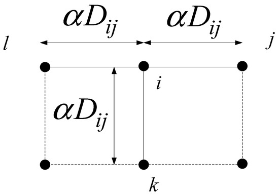
Figure 1. A part of the virtual grid including vertices i, j, k, and l.

The constraint f_i, corresponding to vertex $i$, is written as follows:

$$f_i=x_i+x_j+x_k+x_l\ge 1$$

(4)

3.1. Wind Turbine Placement Prohibition at Specific Locations

Since the grid is virtually constructed, it is possible to have some sites that are not preferable for the installation of wind turbines. The prohibition of wind turbine placement in specific vertices of the grid is related with several parameters such as the different surface conditions, the sheltering effects due to buildings and other obstacles located near the wind farm and the wind variation and intensity which are dependent on by different topographic conditions, e.g., hills and ridges, open plain, sheltered terrain, open sea, and seacoast. Other factors that may prohibit the wind turbine placement is the noise produced by them, the visual impact concerning the neighbouring to private properties or public views, and the influence on areas that have been characterized as archaeological sites or present environmental interest.

When a vertex $i$ is not preferable for the wind turbine installation, the problem of Equation (3) is reformulated as follows:

$$\begin{array}{c}\min {\displaystyle \sum _i{w}_i{x}_i}\\ \mathrm{s}.\mathrm{t}.f(x)\ge \widehat{1}\\ x_i=0,\forall i\in P\\ x\in {\left\{0,1\right\}}^n\end{array}$$

(5)

where the equality constraint x_i = 0 expresses the prohibition of the wind turbine installation at vertex $i$, while $P$ is the set of the prohibited vertices.

3.2. Mandatory Wind Turbine Placement at Specific Locations

The geographical topology presents an important role for the optimal wind turbine installation. Generally, the sites of placement are characterized by high wind potential. Some vertices of the virtual grid, corresponding to specific locations, may have higher wind potential than others. As a result, they are preferable to wind turbine installation. Another classical case for mandatory placement of wind turbines is the case of complex wind farm terrain, where some sites are adequate for placement, and others are sheltered. The distance from loads to be fed is another factor that affects the wind turbine placement, since the cost of wiring becomes prohibitive as the distance increases. Moreover, in cases of older wind farms, some wind turbines must be relocated inside the wind farm to reduce the financial losses.

The mandatory installation of wind turbines is incorporated into the initial problem formulation (3) as

$$\begin{array}{c}\min {\displaystyle \sum _i{w}_i{x}_i}\\ \mathrm{s}.\mathrm{t}.f(x)\ge \widehat{1}\\ x_i=1,\forall i\in L\\ x\in {\left\{0,1\right\}}^n\end{array}$$

(6)

where the equality constraint x_i = 1 expresses the mandatory installation of the wind turbine at vertex $i$, while $L$ is the set of the preferable vertices.

3.3. Microscopic Wind Turbine Placement Considering Local Air Density

For the proper design of a wind farm, many characteristics are considered. One of the most important characteristics is the local climate in terms of the wind speed. Considering the IEC61400-12-1 standard, the normalized wind speed,$V_n$, will be

$$V_n=V{\left(\frac{\rho }{{\rho }_0}\right)}^{1/3}$$

(7)

where ${\rho }_0$ is the reference air density, typically equal to 1.225 kg/m³, and $\rho$ is the local air density at wind turbine hub height. The problem, incorporating the local air density, can be written as

$$\begin{array}{c}\min {\displaystyle \sum _i{V}_{n,}{}_i\left({\rho }_i\right)x_i}\\ \mathrm{s}.\mathrm{t}.f(x)\ge \widehat{1}\\ x\in {\left\{0,1\right\}}^n\end{array}$$

(8)

where $V_{n,i}$ and ${\rho }_i$ are the normalized wind speed and the local air density at wind turbine hub height at vertex $i$, respectively.

4. Simulation Results

Let an area of 5.0625 km². If the blades of wind turbines are 45 m long and the capacity of each turbine is 1.8 MW, a virtual grid with 36 candidate vertices is constructed [26]. Note that the integer number, α, is selected equal to five (α = 5) [27]. The proposed BIP formulation is tested on a 3.4 GHz Intel(R) Core(TM) i7-2600 processor with 16 GB of RAM using the bintprog solver of the MATLAB optimization tool [24]. The bintprog solver uses a linear programming (LP)-based branch-and-bound algorithm. The solution is derived by solving a series of LP-relaxation problems, in which the binary integer requirement on the variables is replaced by the weaker constraint $0\le x\le 1$ [24].

4.1. Wind Turbine Placement without Considering Equality Constraints

Considering the above-described grid and setting the wind turbine installation cost equal to 1 for every vertex i, $w_i=1,\forall i$, the proposed BIP formulation (3) is written as follows:

$$\begin{array}{c}\begin{array}{c}\min {\displaystyle {\sum }_{i=1}^{36}{x}_i}\\ \mathrm{s}.\mathrm{t}.f_i(x)\ge 1,i=1,\dots ,36\end{array}\end{array}$$

(9)

The inequality constraints for vertices 6 and 9 are used for illustration:

$$\begin{array}{l}{f}_6=x_5+x_6+x_{12}\ge 1\\ f_9=x_3+x_8+x_9+x_{10}+x_{15}\ge 1\end{array}$$

(10)

The solution of the above problem gives a total number of ten wind turbines located at vertices 2, 5, 9, 13, 18, 22, 26, 32, 35, and 36. The total installed capacity was 18 MW, while the total time needed to get the final result was 0.132 s. Figure 2 depicts the above-mentioned solution.

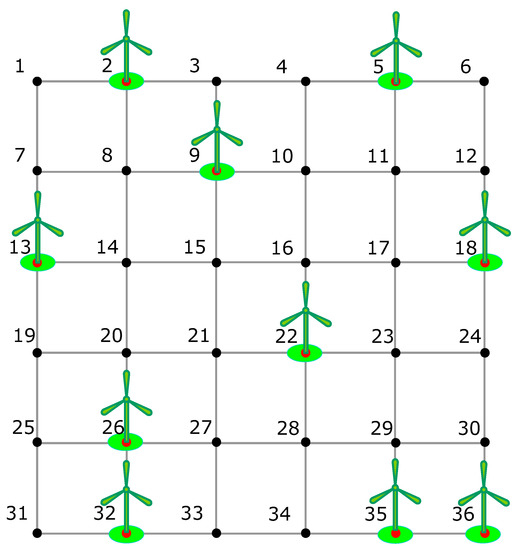
Figure 2. Optimal solution of the wind turbine placement problem without considering equality constraints.

To examine the impact of the integer number α on the performance of the proposed formulation, we conducted simulations considering different values of α for different virtual grid sizes. Table 1 presents the simulation results for different values of α along with the number of vertices in the virtual grid and the corresponding execution time. The last column of the Table 1 includes the ratio of the minimum number of wind turbines to the total number of virtual grid vertices. It is obvious that almost 1/3 of the virtual grid vertices are used for wind turbine installation. Moreover, Figure 3 shows a plot of the objective function value versus iterations to highlight the convergence performance of the proposed formulation for α = 5.

Table 1. Simulation results for different values of α.

α	Virtual Grid Vertices	Minimum Number of Wind Turbines	Execution Time (ms)	λ
5	36	10	132.0	0.278
4	25	7	85.4	0.280
3	16	4	46.8	0.250

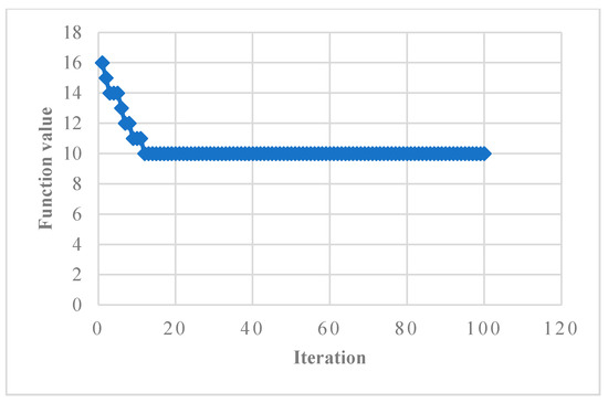
Figure 3. Convergence performance in case without considering equality constraints (α = 5).

4.2. Wind Turbine Placement Prohibition at Specific Locations

The case of wind turbine prohibition is simulated selecting the vertices 18, 19, and 32 of the virtual grid as the locations in which the wind turbine installation is not permitted. According to (5), we can write:

$$\begin{array}{c}\min {\displaystyle \sum _i{w}_i{x}_i}\\ s.t.f(x)\ge \widehat{1}\\ x_{18}=0\\ x_{19}=0\\ x_{32}=0\\ x\in {\left\{0,1\right\}}^{36}\end{array}$$

(11)

The solution of the above problem gives a total number of ten wind turbines located at vertices 3, 6, 7, 11, 16, 20, 24, 27, 31, and 35, while the total installed capacity was 18 MW. The total time needed to get the final result was 0.399 s. Figure 4 presents the problem solution considering the prohibition of wind turbine installation at specific locations.

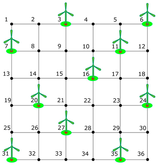
Figure 4. Optimal solution of the wind turbine placement problem considering prohibition at specific locations.

It must be noted that the addition of the three equality constraints in the initial problem formulation increases the time needed to solve the problem and changes the location of wind turbines, while their minimum number remains the same.

4.3. Mandatory Wind Turbine Placement at Specific Locations

The exploitation of higher wind density at specific locations in terms of mandatory wind turbine placement is studied using the model described in (6). Considering that vertices 1, 15, and 34 of the grid, as described in Section 3.2, are more preferable for the wind turbine placement, we can write

$$\begin{array}{c}\min {\displaystyle \sum _i{w}_i{x}_i}\\ s.t.f(x)\ge \widehat{1}\\ x_1=1\\ x_{15}=1\\ x_{34}=1\\ x\in {\left\{0,1\right\}}^{36}\end{array}$$

(12)

The optimal set includes ten wind turbines located at vertices 1, 4, 7, 12, 15, 23, 25, 26, 30, and 34, presented in Figure 5. The total time needed to get the final result was 0.416 s, while the total installed capacity was 18 MW. Once again, the equality constraints added change the wind turbine locations and increase the time needed to solve the problem.

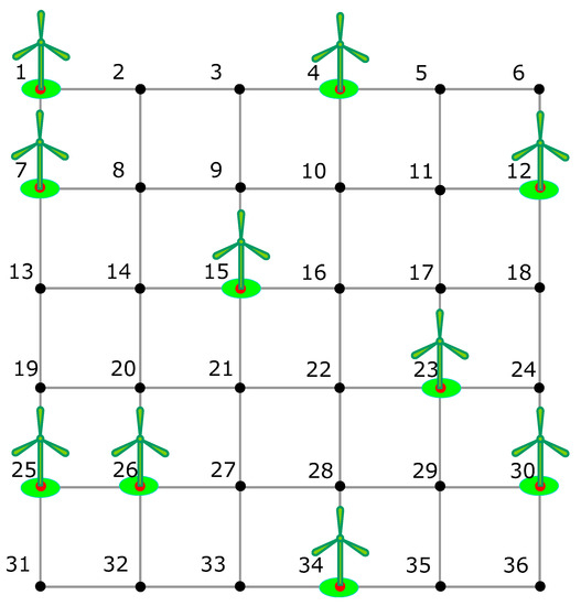
Figure 5. Optimal solution of the wind turbine placement problem considering mandatory wind turbine placement at specific locations.

4.4. Microscopic Wind Turbine Placement Considering Local Air Density

Let the virtual grid of the 36 vertices, where four local areas with different air density existed, namely, A {vertices: 1, 2, 3, 7, 8, 9, 13, 14, 15}, B {vertices: 4, 5, 6, 10, 11, 12, 16, 17, 18}, C {vertices: 19, 20, 21, 22, 23, 24, 29, 30}, and D {vertices: 25, 26, 27, 28, 31, 32, 33, 34, 35, 36}. If the wind speed for each area is 11.00 m/s, 11.20 m/s, 11.10 m/s, and 11.05 m/s, respectively, while the corresponding local air density at wind turbine hub height of each area is 1.199 kg/m³, 1.200 kg/m³, 1.260 kg/m³, and 1.228 kg/m³, the normalized wind speed is calculated for each area, respectively. The optimal wind turbine placement problem considering the local air density at wind turbine hub height will be written as

$$\begin{array}{c}\min {\displaystyle \sum _{i=1}^{36}{V}_{n,}{}_i\left({\rho }_i\right)x_i}\\ \mathrm{s}.\mathrm{t}.f(x)\ge \widehat{1}\\ x\in {\left\{0,1\right\}}^{36}\end{array}$$

(13)

The solution of the above problem gives a total number of ten wind turbines located at vertices 3, 5, 7, 16, 18, 20, 25, 29, 30, and 33, while the total installed capacity was $18\mathrm{{\rm M}}\mathrm{W}.$ The total time needed to get the final result was 0.423 s.

To consider the geographic topology and the wind data using a real case, we selected a geographical territory in Skyros island, Greece. Skyros island belongs to Northern Sporades and covers an area of 308 km². In this case, we incorporated also the mandatory placement and prohibition of wind turbine’s placement. Figure 6 presents in the left hand the wind data as they received from Centre of Renewable Energy Sources & Saving (CRES) [28], while the right hand of the figure presents the geographic morphology of the island. Considering the morphology of the area, the wind potential, the length of wind turbines’ blades (each blade is 45mlong), and that the integer number α is equal to 5, a squared area of 20.25 km² is constructed including 121 candidate vertices (yellow squared area in Figure 6). Considering also that six candidate vertices are excluded due to lower wind potential and four other vertices are mandatory selected due to the highest wind potential, the implementation of the proposed algorithm gave as a result 42 wind turbines, while the execution time was 1.475 s.

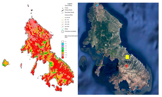
Figure 6. Wind data and geographic topology of Skyros island, Greece.

4.5. Comparison with Other Works in the Literature

In order to demonstrate the efficiency of the proposed algorithm regarding wind turbine placement, Table 2 compares the results for cases described in Section 4.1 and Section 4.2, in terms of wind turbines number, locations, and execution time, with the corresponding results of [26]. For the sake of simplicity, we name the case in which equality constraints are not considered in the problem formulation as Case 1 and the case in which the wind turbine placement at specific locations is prohibited as Case 2, respectively. As can be seen, for all cases, the proposed method provides equal number of wind turbines, but in different locations. Moreover, the execution time is quite similar. The difference between the execution times included in Table 1, for Cases 1 and 2, is related with the introduction of additional equality constraints to the problem formulation, increasing the complexity of the problem as well as the corresponding execution times.

Table 2. Comparison of the proposed BIP method with work [26].

36-Nodes Grid	Proposed BIP Method			Method [26]
	Wind Turbines Number	Wind Turbines Location	Execution Time (s)	Wind Turbines Number	Wind Turbines Location	Execution Time (s)
Case 1	10	2, 5, 9, 13, 18, 22, 26, 32, 35, and 36	0.132	10	2, 5, 8, 16, 18, 19, 21, 29, 32, and 35	0.128
Case 2	10	3, 6, 7, 11, 16, 20, 24, 27, 31, and 35	0.399	10	3, 6, 7, 11, 14, 22, 24, 25, 33, and 35	0.390

Given that the rated power of each wind turbine is $1.8\mathrm{{\rm M}}\mathrm{W}$ and considering that the capacity factor is $0.26,$ the annual energy production of the wind turbine used, will be 0.26·1.8·8760 = 4100 MWh/year. Since the optimal solution, for each simulated case, includes 10 identical wind turbines of the same vendor, the annual energy production of the wind farm will be 41,000 MWh/year. Moreover, considering that the total installation cost, including turbine (ex-works), foundation, electric installation, grid connection, control systems, consultancy, land, financial costs, and road, is 1000 EUR/MW [29], the total installation cost for wind turbines will be 10·1.8·1000 = 18,000 EUR.

Table 3 provides a summary of the variables and settings used for the simulations, while a qualitative comparison of the proposed method with other works published in the literature in terms of the contribution is presented in Table 4.

Table 3. Summary of the data used for the simulation of the 36-nodes virtual grid.

Data	Values
Area	5.0625 km2
Length of wind turbine’s blades	45 m
Wind turbine’s capacity	1.8 MW
Integer number to avoid wake effect	5
Capacity factor	0.26

Table 4. Qualitative comparison of the proposed BIP method with other works in the literature.

Method	Contribution
[3]	The problem is addressed in discrete space by considering a gridded version of the wind farm site and designating the corresponding cell centers as candidate wind turbine locations. The problem is solved using a genetic algorithm.
[4]	A scheme for rare positioning of the wind turbines that significantly reduces the land requirements through higher density of turbines is proposed.
[5]	The primary goal of this work is to link boundary-layer and turbine wake models for the better determination of the wind shear and turbulence profiles inside large offshore wind farms.
[6]	A genetic algorithm approach is proposed to minimize the number of turbines installed and maximize the production capacity considering non-uniform wind with variable direction, uniform wind with variable direction, and unidirectional uniform wind.
[8]	A Weibull distribution is used to commonly approximate the wind speed probability density function at a site to correctly calculate the wind turbine power generating capability.
[7,9]	Different algorithms for the wind turbines placement, namely, gradient search algorithm (GSA), greedy heuristic (GHA), genetic (GA), simulated annealing (SAA), and pattern search (PSA), are examined in terms of the computation time needed to get the optimal solution and the quality of the solution.
[10]	An approach based on Monte Carlo simulation to maximize the energy production and minimize installation cost criteria is proposed.
[11]	This proposal optimizes the locations of each turbine within its cell boundaries in terms of maximizizng the generated wind power considering real-coded genetic algorithms.
[12]	An approach for wind farm design, based on evolutionary algorithms and related techniques emphasizing particle swarm optimization.
Proposed	A given territory is subdivided into squares considering the wake effect and constructing a virtual grid to find the optimum allocated wind turbines for this grid. The avoidance of the wake effect is achieved considering a minimum distance between the wind turbines. The effect of local air density is also considered for the microscopic placement of wind turbines.

5. Conclusions

This paper proposes an efficient method for wind turbine placement in power plants, by using a binary integer programming approach. Additional equality constraints are also included to the proposed formulation in order to prohibit or enforce the installation of wind turbines placement at specific locations of the wind farmland. Data related with the area of geographical territory, the length of wind turbine blades, and the capacity of each turbine were used for more-realistic simulations. A microscopic wind turbine placement considering the local air density was also studied. The suggested formulation was tested in MATLAB environment using the bintprog solver and a 36-nodes virtual grid, while a real case scenario concerning the Greek island of Skyros was also examined. The simulation results were compared in terms of wind turbines number, locations, and execution time, with those of a previous author’s work. The results showed that the proposed methodology can be effectively implemented considering or prohibiting the installation of wind turbines in specific locations. The execution time needed is comparable with that of a previously published work, while the minimum number of wind turbines is the same.

References

- Jacobson, M.Z.; Delucchi, M.A. Providing all global energy with wind, water, and solar power, Part I: Technologies, energy resources, quantities and areas of infrastructure, and materials. Energy Policy 2011, 39, 1154–1169. [Google Scholar] [CrossRef]
- Patel, M.R. Wind and Solar Power Systems; CRC Press: Boca Raton, FL, USA, 1999. [Google Scholar]
- Mosetti, G.; Poloni, C.; Diviacco, B. Optimization of wind turbine positioning in large wind farms by means of a genetic algorithm. J. Wind Eng. Ind. Aerodyn. 1994, 51, 105–116. [Google Scholar] [CrossRef]
- Ammara, I.; Leclerc, C.; Masson, C. A Viscous Three-Dimensional Differential/Actuator-Disk Method for the Aerodynamic Analysis of Wind Farms. J. Sol. Energy Eng. 2002, 124, 345–356. [Google Scholar] [CrossRef]
- Barthelmie, R.; Larsen, G.; Pryor, S.; Jørgensen, H.; Bergström, H.; Schlez, W.; Rados, K.; Lange, B.; Vølund, P.; Neckelmann, S.; et al. ENDOW (efficient development of offshore wind farms): Modelling wake and boundary layer interactions. Wind Energy 2004, 7, 225–245. [Google Scholar] [CrossRef]
- Grady, S.; Hussaini, M.; Abdullah, M. Placement of wind turbines using genetic algorithms. Renew. Energy 2005, 30, 259–270. [Google Scholar] [CrossRef]
- Elkinton, C.N.; Manwell, J.F.; McGowan, J.G. Algorithms for Offshore Wind Farm Layout Optimization. Wind. Eng. 2008, 32, 67–84. [Google Scholar] [CrossRef]
- Lackner, M.A.; Elkinton, C.N. An Analytical Framework for Offshore Wind Farm Layout Optimization. Wind. Eng. 2007, 31, 17–31. [Google Scholar] [CrossRef]
- Elkinton, C.N.; Manwell, J.F.; McGowan, J.G. Optimization algorithms for offshore wind farm micrositing. In Proceedings of the Windpower Conference and Exhibition, Los Angeles, CA, USA, 3–6 June 2007. [Google Scholar]
- Marmidis, G.; Lazarou, S.; Pyrgioti, E. Optimal placement of wind turbines in a wind park using Monte Carlo simulation. Renew. Energy 2008, 33, 1455–1460. [Google Scholar] [CrossRef]
- Wan, A.; Wang, J.; Yang, G.; Zhang, X. Optimal siting of wind turbines using real-coded genetic algorithms. In Proceedings of the European Wind Energy Association Conference and Exhibition, Marseille, France, 16–19 March 2009. [Google Scholar]
- Wan, C.; Wang, J.; Yang, G.; Zhang, X. Optimal Micro-siting of Wind Farms by Particle Swarm Optimization. Comput. Vision 2010, 6145, 198–205. [Google Scholar] [CrossRef]
- Mora, J.C.; Barón, J.M.C.; Santos, J.M.R.; Payán, M.B. An evolutive algorithm for wind farm optimal design. Neurocomputing 2007, 70, 2651–2658. [Google Scholar] [CrossRef]
- Kusiak, A.; Song, Z. Design of wind farm layout for maximum wind energy capture. Renew. Energy 2010, 35, 685–694. [Google Scholar] [CrossRef]
- Mustakerov, I.; Borissova, D. Wind turbines type and number choice using combinatorial optimization. Renew. Energy 2010, 35, 1887–1894. [Google Scholar] [CrossRef]
- Anescu, G. Optimal placement of wind turbines using NSC-PSO algorithm. In Proceedings of the 2016 International Symposium on INnovations in Intelligent SysTems and Applications (INISTA), Sinaia, Romania, 2–5 August 2016; pp. 1–8. [Google Scholar]
- Hendrawati, D.; Soeprijanto, A.; Ashari, M. Optimal power and cost on placement of Wind turbines using Firefly Algorithm. In Proceedings of the 2015 International Conference on Sustainable Energy Engineering and Application (ICSEEA), Bandung, Indonesia, 5–7 October 2015; pp. 59–64. [Google Scholar]
- Hou, P.; Hu, W.; Soltani, M.N.; Chen, C.; Zhang, B.; Chen, Z. Offshore Wind Farm Layout Design Considering Optimized Power Dispatch Strategy. IEEE Trans. Sustain. Energy 2016, 8, 638–647. [Google Scholar] [CrossRef]
- Lamaina, P.; Sarno, D.; Siano, P.; Zakariazadeh, A.; Romano, R. A Model for Wind Turbines Placement Within a Distribution Network Acquisition Market. IEEE Trans. Ind. Inform. 2015, 11, 210–219. [Google Scholar] [CrossRef]
- Manjarres, D.; Sanchez, V.; Del Ser, J.; Landa-Torres, I.; Gil-Lopez, S.; Walle, N.V.; Guidon, N.; Sánchez, V. A novel multi-objective algorithm for the optimal placement of wind turbines with cost and yield production criteria. In Proceedings of the 2014 5th International Renewable Energy Congress (IREC), Hammamet, Tunisia, 25–27 March 2014; pp. 1–6. [Google Scholar]
- Marseglia, G.; Arbasini, A.; Grassi, S.; Raubal, M.; Raimondo, D. Optimal placement of wind turbines on a continuous domain: An MILP-based approach. In Proceedings of the 2015 American Control Conference (ACC), Chicago, IL, USA, 1–3 July 2015; pp. 5010–5015. [Google Scholar]
- Mokryani, G.; Siano, P. Strategic placement of distribution network operator owned wind turbines by using market-based optimal power flow. IET Gener. Transm. Distrib. 2014, 8, 281–289. [Google Scholar] [CrossRef]
- Siano, P.; Mokryani, G. Assessing Wind Turbines Placement in a Distribution Market Environment by Using Particle Swarm Optimization. IEEE Trans. Power Syst. 2013, 28, 3852–3864. [Google Scholar] [CrossRef]
- Matlab. Version 8.3 (Release 2014a); MathWorks: Natick, MA, USA, 2014. [Google Scholar]
- Luenberger, D.G.; Ye, Y. Linear and Nonlinear Programming, 3rd ed.; Springer Science Business Media, LLC: New York, NY, USA, 2008. [Google Scholar]
- Manousakis, N.M.; Psomopoulos, C.S.; Ioannidis, G.C.; Kaminaris, S.D. Optimal placement of wind turbines using sem-idefinite programming. In Proceedings of the Mediterranean Conference on Power Generation, Transmission, Distribution and Energy Conversion (MEDPOWER), Belgrade, Serbia, 6–9 November 2016. [Google Scholar]
- Ituarte-Villarreal, C.M.; Espiritu, J.F. Optimization of wind turbine placement using a viral based optimization algorithm. Procedia Comput. Sci. 2011, 6, 469–474. [Google Scholar] [CrossRef]
- CRES. Available online: http://www.cres.gr/cres/index.html (accessed on 1 April 2021).
- Wind Energy—The Facts. Available online: https://www.wind-energy-the-facts.org/ (accessed on 1 April 2021).
Publisher’s Note: MDPI stays neutral with regard to jurisdictional claims in published maps and institutional affiliations. |
© 2021 by the authors. Licensee MDPI, Basel, Switzerland. This article is an open access article distributed under the terms and conditions of the Creative Commons Attribution (CC BY) license (https://creativecommons.org/licenses/by/4.0/).