Three-Dimensional Analysis for the Documentation of the Restoration of an Earthquake-Damaged Triptych

Abstract

The 3D digital reproduction of panel paintings is an efficient practice through which to document their state of conservation thanks to the ability to study artwork both at the microscopic level, visualising the craquelure and the detachments of pictorial layers, and at the macroscopic level, analysing support structures and their deformations. In recent years, research has focused on new methodologies to handle multiple 3D scans acquired over time and to achieve data fusion to obtain multi-resolution products. In this paper, we present the results of the acquisition of the central panel of an earthquake-damaged triptych using two different 3D techniques (close-range photogrammetry and structured light) before and after its restoration to carry out a multi-temporal analysis of the conservation status and document the effects of the restoration. Furthermore, we performed laser scanning micro-profilometry on a small area of the painting to study the artist’s technique and identify previous restorations. Finally, we merged the two 3D datasets (obtained by structured-light projection and micro-profilometry) to produce a multi-resolution 3D model with the aim of increasing the accuracy and readability of the final product.

1. Introduction

The 3D digitisation of cultural heritage is valuable in conservation, preservation, reproduction, research, creative and tourism-related applications.

In the case of cultural heritage that is at risk of being lost by sudden events such as disasters or theft, as well as more long-term and continuous processes, e.g., climate change and the continuous use and natural decay of materials, 3D digitisation is a necessity for not only its preservation, conservation and material analysis but also for restoration purposes.

Three-dimensional models aid conservators in studying artwork, making hypotheses of integrations through virtual simulation [1], providing a reference for the integration of data collected with other diagnostic techniques and the creation of high-accuracy copies in a non-invasive and no-contact way [2]. The digitalisation of an artwork provides a 3D model of its current conservative state that enables the extraction of quantitative information both at a structural (e.g., cracks) and morphological (e.g., roughness) level.

Restrictions on public access due to the total closure of museums during the pandemic emergency brought the problem of the remote fruition of works of art back to the fore. From this perspective, 3D surveys played a central role; since then, the development of tools for the virtual fruition of museums and archaeological sites using interactive and immersive remote tours has increased, accounting not only for restrictions to the number of visitors but also for access limitations for people with disabilities [3].

In recent years, restorers have recognised the potential and usefulness of 3D documentation, making the creation of 3D models a good practice in many restoration projects. As an example, solutions related to the use of 3D models and data mapping on 3D surfaces in the context of documentation in a complex intervention are described in ref. [4]. The monitoring of shape variations over time to keep trace of deformations due to thermo-hygrometric changes, the surface weathering of outdoor objects, damage caused by natural disasters or the effects of restoration work is a challenging issue. Robson et al. [5] applied photogrammetry for the periodic high-precision monitoring of a panel painting during the conservation process. Bratasz et al. [6] monitored the responses of a variety of sculpted wooden elements to variations in temperature and relative humidity in their environment using triangulation laser displacement sensors. Guidi et al. [7] tested the use of 3D imaging technology to monitor wooden artworks when sudden changes occur in environmental parameters. Hess et al. [8] demonstrated the potential of 3D colour laser scanning to monitor the dimensional stability of a Byzantine ivory panel. Palma et al. [9] proposed a new method to quantify panel deformations, based on a non-rigid registration algorithm, by comparing 3D models acquired with different scanning devices and at different times (2002 and 2015).

It is thanks to technological development that 3D surveys have moved from being a mere architectural and archaeological application to including the surveyal of nearly flat objects such as paintings [10,11,12,13]. In addition to structural analysis at the macroscopic level [10,14], high-resolution 3D techniques make it possible to study surface details such as craquelure, paint detachments and any irregularities in the protective layer [15,16] at a microscopic level. The technique best suited for a specific task depends on several factors, such as the object dimensions and the resolution required, but rarely can a single technique satisfy all the requirements.

Therefore, it is often necessary to use different instruments with different gauge volumes and resolutions and then integrate the results. Data merging, also called data fusion or data integration [17], is the process of integrating multiple raw data to produce more consistent, accurate and useful information than that provided by any individual data source. In addition to being more informative, fused data are more compressed than the original inputs [18]. In the cultural heritage field, an example of data fusion is the integration of image-wise (2D) data such as UV fluorescence, visible and IR reflectography imaging with digital models (3D data) [19,20,21,22], as well as the integration of 3D models derived from different techniques [23,24].

This work focuses on the study of the central panel of a triptych that was severely damaged in the 2016 earthquake that shook central Italy, which is still under repair at the Restoration Laboratories of the Opificio delle Pietre Dure in Florence. The painting was in a truly dreadful conservation state: the collapse of the roof of the Church of San Vittorino—in the small village of Nocria, a hamlet in the municipality of Castelsantangelo sul Nera, in the province of Macerata, in the Marche region—caused extensive damage to the artworks preserved inside, including the triptych located on the wall of the main altar. Upon its arrival at the Opificio, the central panel showed a vertical break spanning more than half the length of the board and a horizontal break on the upper-right side, at the crossbeam, where the wood fibres of the support had broken and stretched, undergoing irreversible deformation. The degradation phenomena of the painted surface, such as detachments of the pictorial layers, were closely linked to the problems related to the support and the deformations caused to the panel by the earthquake. Furthermore, there were colour gaps, abrasions, scratches and dimplings in the paint film caused by the collision of rubble from the church.

The restoration of the support consisted of the integration and consolidation of detached elements, smoothing/cohesion of the detachments, re-joining of the cracks and replacement of the old rigid crossbeams with new ones equipped with springs to follow the natural movements of the wooden support.

The 3D model, therefore, stands as the only evidence of the conservation status of the panel before the restoration intervention. Moreover, it is a valuable tool for measuring the cracks and rifts and quantifying the structural deformations. Furthermore, to document the effects of restoration, the panel shape was also acquired after the repair intervention. We used two different 3D techniques for the 3D survey before and after the restoration, close-range photogrammetry and structured-light projection, respectively, the choice of which was imposed by the availability of the instruments at the time of the acquisition, given the better resolution of structured-light projection than photogrammetry. The main aims of this work were the multi-temporal monitoring of the conservative state of the painting before and after the restoration and the documentation of the shape variations in the panel due to the intervention. Indeed, the research focused on new methodologies to handle multiple 3D scans acquired over time. Finally, we showed the multi-resolution 3D model of the painting created by fusing the 3D data acquired by the structured-light scanner and micro-profilometry. The latter was used to acquire details of the painting to produce a high-resolution map to study the artist’s technique and identify previous restorations.

2. Materials and Methods

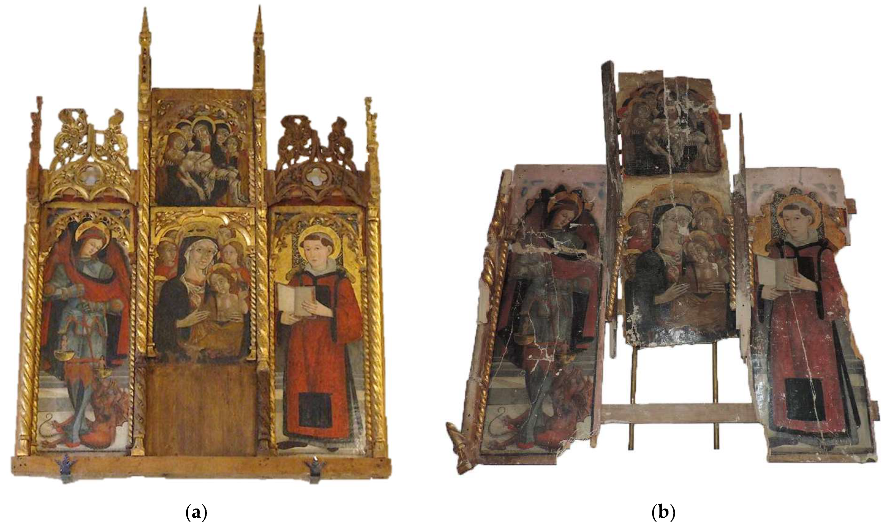
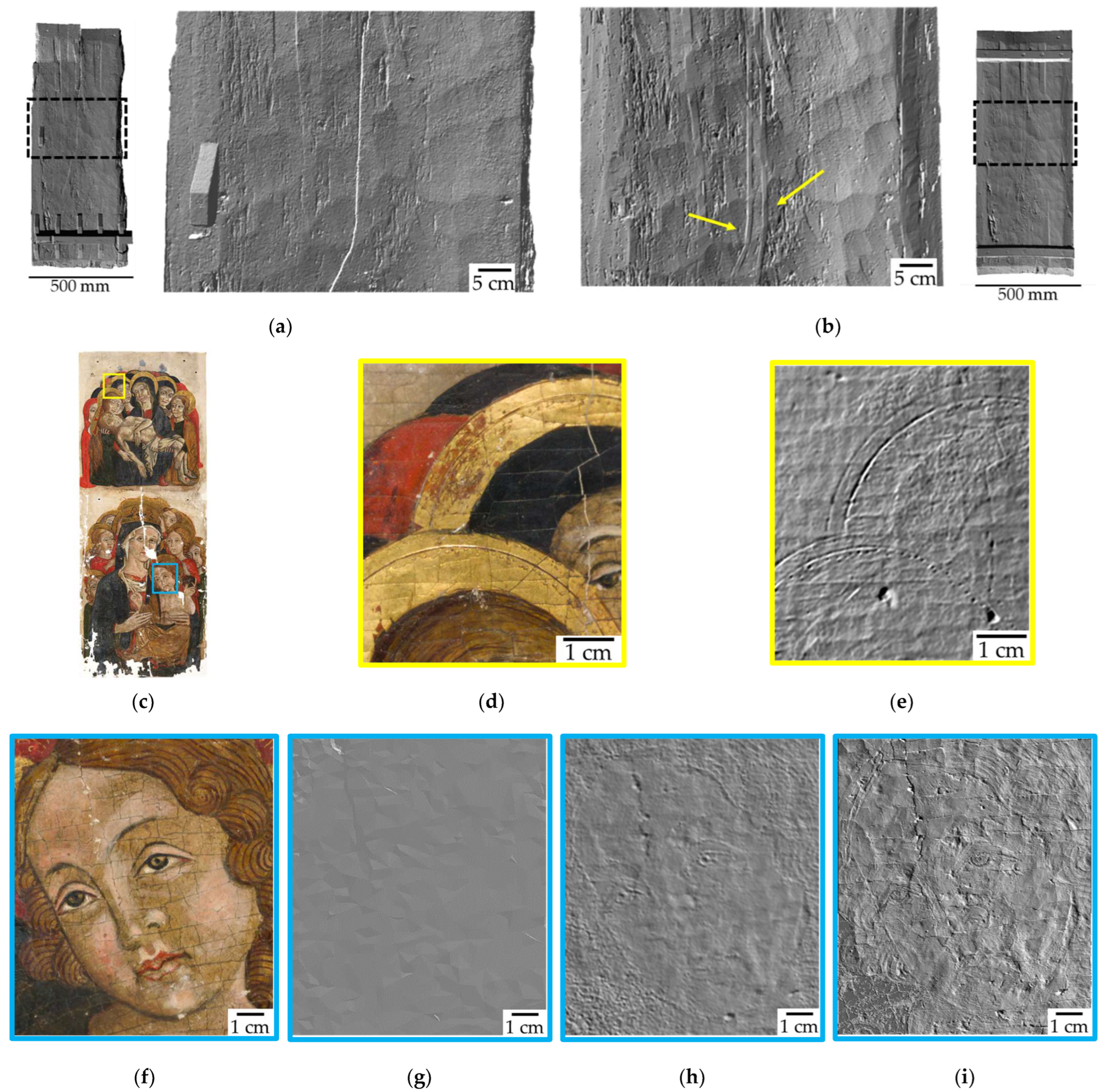
2.1. Case Study

The painting under examination was the central panel of a late gothic triptych (Figure 1), dating around 1480–1490, made for the main altar of S. Vittorino church in Nocria. The artwork is attributed to local painters from the circle of Paolo da Visso, the most important painter from the area. Its history is rather complex: it has been moved several times within the church, and in addition to the damage and destruction of some elements caused by the earthquake, the work has undergone modifications over time that have altered its shape and dimensions; a previous restoration dating 1970–1971 has been documented [25].

The triptych is a tempera painting composed of three wooden panels (120 cm × 45 cm each) separated by twisted columns in a gilded wooden frame (overall dimensions: 207 cm × 150 cm). The central panel is made of two sections: the upper one depicts the Madonna holding the Dead Christ with St. Mary Magdalene and St. John; the lower one shows the Crowned Madonna and the Child surrounded by angels. The side panels depict St. Michael the Archangel on the left and a saint deacon and martyr on the right [26].

The critical conservation status of the wooden support due to the seismic event made it necessary to firstly consolidate the panels and integrate the detached elements and secondly replace the old rigid crosspieces with new ones to accommodate the natural movement of the wood.

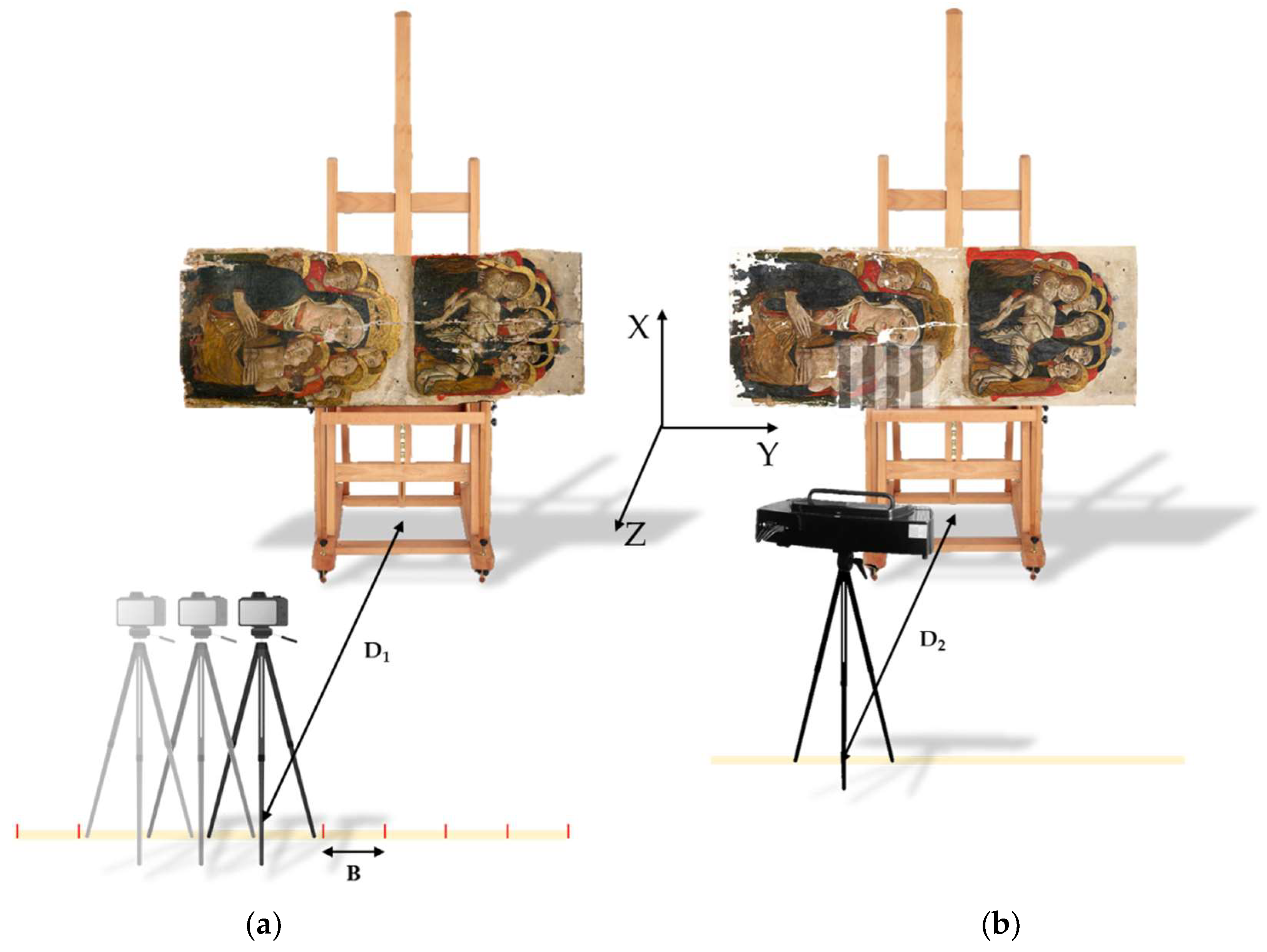
2.2. Close-Range Photogrammetry

Photogrammetry is the science of making accurate measurements from photographs and using optics’ principles, the internal parameters of a camera and its orientation to reconstruct dimensions and positions of objects from overlapping images [27].

Therefore, photogrammetry is a technique based on the triangulation principle that produces 3D metric models from 2D image acquisitions (called photograms) taken from different angles and positions. It is a passive technique where the source is sunlight or ambient light for outdoor and indoor measurements, respectively. Originally created for architectural and archaeological surveys, photogrammetry is used, at present, in several fields with different stand-off distances and resolutions, e.g., from micro-photogrammetry (images acquired with a stereo-microscope) to aerial photogrammetry (from a satellite or a UAV). Close-range photogrammetry, with stand-off distances between 1 and 30 m, is widely used in the cultural heritage field [28] and has been fruitfully applied to the study of paintings and the documentation of repair interventions [5,14,29].

We performed close-range photogrammetry for the survey of the panel before restoration using a full-frame NIKON D850 digital reflex camera with a CMOS sensor (35.9 mm × 23.9 mm, 4.35 µm pixel size and 46 Mpx resolution). The camera, mounted on a Manfrotto tripod, was equipped with a Nikkor 60 mm objective lens, and each image was acquired with the following settings: ISO 200, f/25 aperture and 1/250 s exposure time. Two Yongnuo Speedlite YN685 flashes were set at 45° from the panel surface and were moved together with the camera; the lightened area was much bigger than the shooting one so that the lighting could be considered almost uniform. To make colours appear more realistic, we performed white balance adjustment by using a 99% Spectralon White diffuse reflectance standard placed in the acquisition area.

The panel was placed on an easel, which did not allow for the acquisition in continuum; therefore, we carried out two separate shooting sessions, one on the front (152 images) and one on the back (147 images) of the panel, and the two different data sets were processed separately, resulting in two distinct 3D models.

For all shoots, we maintained the same measurement set-up (Figure 2a) by keeping both the object-to-camera distance (D₁) and the baseline (B), i.e., the distance between two consecutive acquisitions, constant. The latter was set to ensure at least 70% overlap between two successive images.

The image processing and the creation of the 3D model followed the typical photogrammetric workflow [30], which was carried out using Agisoft Metashape software (v.2.0.4, https://www.agisoft.com/, accessed on 10 October 2022) based on the Structure from Motion (SfM) and Dense Multi-View 3D Reconstruction (DMVR) algorithms.

Before starting the alignment, in each photogram, out-of-interest areas (e.g., the background and easel) were masked and removed to speed up the processing and make it easier.

After the identification of homologous points (key or tie points) necessary for the matching of consecutive images, the algorithm generated a sparse cloud (Figure 3a), i.e., a low-density point cloud that contains the 3D coordinates of the characteristic points in a shared coordinate system. Subsequently, the sparse cloud was converted into the real scale and referenced to an XY system through the input of known distances measured on the object (scale bars) to generate a dense point cloud (Figure 3b), i.e., a set of a large number of points that reproduces the real object. Afterwards, the recovered point cloud was triangulated and the mesh, a triangular 3D model with a continuous and structured surface, was generated (Figure 3c). Finally, the textured realistic model was obtained through the application of the texture on the mesh (Figure 3d).

Metrics

To evaluate the spatial resolution of the photogrammetric 3D models, we considered the Ground Sampling Distance (GSD), defined as the distance between the centre of two adjacent pixels on the object. The GSD is the projection of the camera pixel on the object space, and it is the smallest element that can be detected and reconstructed in 3D [31,32], as follows:

$$GSD=\frac{D·d }{f }$$

(1)

where D is the camera-to-object distance, d is the camera pixel size and f is the focal length. We set D = 115 cm, and with $d$ = 4.35 µm and $f$ = 60 mm, the GSD was 83.4 µm.

In the case of canonical configuration, also called a ‘normal case of stereo-photogrammetry’ [33], the camera optical axis is perpendicular to both the baseline and the object surface, and the depth resolution $\left(dz\right)$ can be expressed as follows [34,35,36]:

$$dz=\frac{D^2·d}{Bf-Dd }$$

(2)

The baseline B was set to 20.7 cm, resulting in a depth resolution $dz$ of 463 µm.

The theoretical precision σ is the expected variability in estimated 3D object coordinates [31] and depends on the ratio of the camera-to-panel distance to the focal length, known as the frame scale ($S_f=\frac{D}{f}$), and on the image measurement accuracy (${\sigma }_{X^{\prime }}$).

The in-plane theoretical precision $({\sigma }_X$ and ${\sigma }_Y$) is expressed by the following:

$${\sigma }_X={\sigma }_Y=\frac{D}{f}{\sigma }_{X^{\prime }}$$

(3)

We supposed an image measurement accuracy ${\sigma }_{X^{\prime }}$ of 0.5 pixels (2.175 µm) [37,38]; therefore, the resulting in-plane precision ${\sigma }_X={\sigma }_Y$ was 41.2 µm.

The axial theoretical precision ${\sigma }_Z$ (along the Z direction), besides depending on the frame scale, is a function of the baseline, as follows:

$${\sigma }_Z=\frac{D^2}{f·B}{\sigma }_{p{X}^{\prime }}$$

(4)

where ${\sigma }_{p{X}^{\prime }}$ is the image measurement accuracy of the x-parallax, and it was assumed that ${\sigma }_{X^{\prime }}=$ ${\sigma }_{p{X}^{\prime }}$. The axial precision was then 232 µm.

The overall precision of a 3D point measurement $\left({\sigma }_{XYZ}\right)$ is then given by the following:

$${\sigma }_{XYZ}=\sqrt{{\sigma }_X^2+{\sigma }_Y^2+{\sigma }_Z^2}$$

(5)

and was equal to 239 µm. All resolution and theoretical precision values are summarised in

Table 1. Model accuracies calculated with D = 115 cm, f = 60 mm, B = 20.7 cm and d = 4.35 µm.

GSD Ground Sampling Distance [µm]	dz Depth Resolution [µm]	${\mathit{\sigma }}_{{\mathit{X}}^{\prime }}$ Accuracy in Image Space [µm]	${\mathit{\sigma }}_{\mathit{X}}={\mathit{\sigma }}_{\mathit{Y}}$ In-Plane Theoretical Precision [µm]	${\mathit{\sigma }}_{\mathit{Z}}$ Axial Theoretical Precision [µm]	${\mathit{\sigma }}_{\mathit{X}\mathit{Y}\mathit{Z}}$ Overall Precision [µm]
83.4	463	2.175	41.2	232	239

.

2.3. Structured-Light Projection

Structured light is an active technique based on the projection of non-coherent light patterns (coloured or monochromatic fringes) that are distorted by the surface morphology and acquired by one or two cameras. The object’s shape is recovered by triangulation once the baseline, i.e., the distance between the camera and the projector, and their orientation, i.e., the angles at either end of the baseline, are known [39,40].

In this work, we used the MICRON3D colour structured-light scanner (SMARTTECH 3D), mounted on a stable tripod with a tilt head. The scanner is equipped with a white LED projection system with variable spatial frequency and direction fringes and two lateral CCD cameras. Each instrument detector has 18 Mpx; the field of view is 30 cm × 40 cm with a depth of field of about 20 cm; the distance between points is 80 µm; the density is 150 pp/mm²; and the accuracy is 60 µm.

The technology used in the MICRON3D colour scanner (SMARTTECH3Dmeasure proprietary software, v.23) allows for the simultaneous measurement of an object’s surface into the cloud of points with XYZ spatial coordinates and RGB colour values assigned.

To avoid excessive memory overload on the computer and for rapid data processing, the Simplified Mode option was used for all acquisitions, resulting in 25% of the full resolution of the Precise Mode modality. For the best-quality coloured point cloud that precisely reproduced the characteristics of the object’s surface and to avoid shaded areas, an automatic shadeless lighting system was used.

The panel-to-instrument distance was set to 70 cm, and the painting was placed on an easel and properly moved to acquire the front, the back and the edges, for a total of 49 acquisitions (Figure 2b). After cleaning to remove the noise and undesired points, the point clouds were aligned using the three homologous points method to create a single point cloud (81,404,830 points). The point cloud was then transformed into a triangle mesh (12,988,936 vertices and 25,932,924 faces, Figure 4a,b,e) and, finally, the texture was applied (Figure 4c,d,f).

2.4. Laser Scanning Micro-Profilometry

The optical micro-profilometer is an in-house laser scanning device developed at INO-CNR [41,42,43,44,45]. The instrument is made of a commercial probe (Conoprobe 1000 by Optimet, Jerusalem, Israel) mounted on a high-resolution XY scanning system with a precision of 0.1 μm and a maximum scanning area of 30 × 30 cm². The scanning speed ranges from 100 to 400 points/s depending on the acquisition parameters (sampling step and maximum travel length), and the whole system is computer controlled. The probe can be equipped with a set of lenses with different focal lengths. In this work, we used the 50 mm lens to analyse the surface morphology to assess the detachments, craquelure, flakes, wrinkles and grooves in the pictorial and preparatory layers. This focal length provides a working distance of 40 mm and a dynamic range of 8 mm, making it suitable for shape measurements of nearly flat surfaces. The axial resolution is 1 µm, the overall accuracy is 6 µm and the maximum transversal resolution is 20 µm. We scanned an area of 90 × 105 mm², representing the Child’s face, with a 50 µm sampling step. The output was a high-resolution topographic map that could be displayed as a 3D model or as a grey- or colour-scale image that could be further elaborated through the application of digital filters to simulate the direction of the impinging light, resulting in an image very similar to the traditional raking light photo.

3. Results

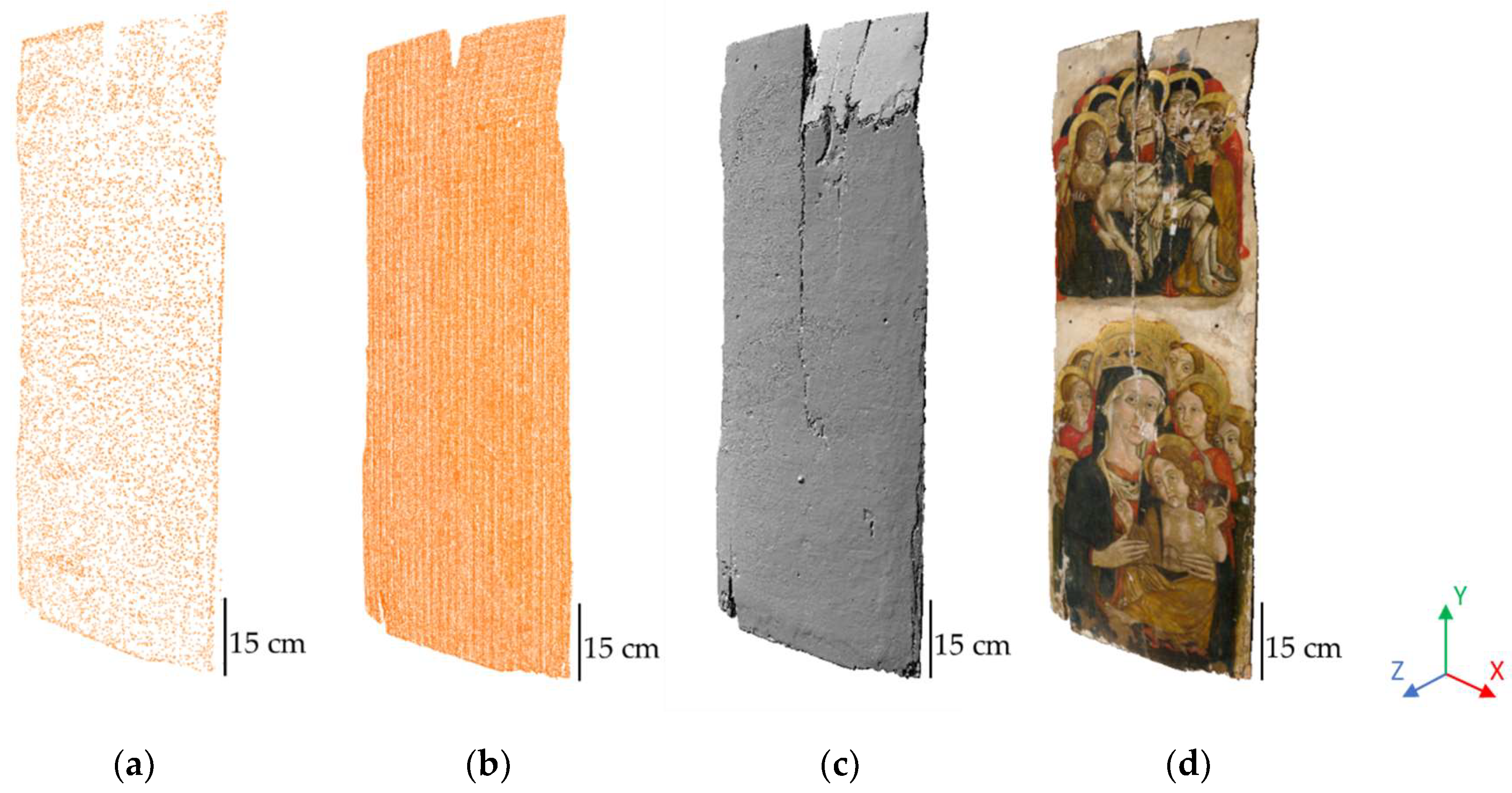
3.1. Three-Dimensional Data-Quality Evaluation

Presently, there are plenty of 3D techniques that have become part of the diagnostics of works of art. Their applicability to different conservation situations depends on their performance in terms not only of resolution but also the gauge volume/area, acquisition time and cost of the instrumentation. Investigation before restoration often requires both a comprehensive and a detailed analysis of the artwork, thus necessitating a multi-modal and multi-resolution approach to assess all issues. Moreover, data are often collected with different sensors at different times in variable contexts [46]. Therefore, understanding the quality of 3D results is essential to know what information can be extracted from 3D models obtained from different instruments. Concerning the study of the painting under investigation, techniques with different performances were applied to assess the effects of degradation due to the earthquake at both the macroscopic (structural) and microscopic (pictorial layer) levels. The quality of the acquired datasets is discussed in the following section. Point density is one of the parameters that determines the quality of the geometry of a 3D mesh when it is consistent and accurate with the geometry of the objects represented [47]. Defined as the number of points per area, it is directly related to point spacing; therefore, the closer the point groups, the higher the point density [48]. We performed the density calculation to qualify the 3D models obtained in this work. To this end, we used a CloudCompare tool (https://www.danielgm.net/cc/, 13 January 2024, v.2.12.4) that estimates the density following the formula $density=\frac{N}{\pi R^2}$, where N is the number of neighbours, for each point, within a sphere of radius R. We set R = 0.5 mm for all point clouds, and the results for the data of the front panel after restoration are summarised in

Table 2. Details of the point clouds and meshes obtained with photogrammetry, structured-light scanner and micro-profilometer.

	Techniques	Sampled Area [cm2]	Number of Points	Number of Vertices	Number of Faces	Point Density with R = 0.5 mm [pp/mm2]
Pre-restoration (front)	Photogrammetry	45 $\times$ 120	6,380,304	80,762	160,369	12 ± 1
Post-restoration (front)	Structured-light topography	45 $\times$ 120	35,634,635	6,013,775	12,007,973	74 ± 29
Child’s face	Micro-profilometry	9 $\times$ 10.5	3,609,905	3,609,905	7,176,312	384 ± 29

for comparison with the photogrammetric front model before restoration. The surface density of the pre-restoration dense cloud is consistent with the GSD calculated for the photogrammetry spatial resolution.

Figure 5 displays some details of the models without texture to compare the Levels of Detail (LODs) achieved by the three techniques in this case study. In the back side of both the pre- and post-restoration models, adze marks are clearly visible (Figure 5a,b), but the traces of woodworking are better defined in the latter due to the higher resolution of the structured-light scanner. Furthermore, in the post-restoration model, traces of holes caused by xylophagous insects appear.

The pre-restoration model shows a vertical crack, which was repaired by adding wooden inserts that can be seen in the post-restoration model (indicated by two yellow arrows in Figure 5b).

The 3D model of the panel front side created by the structured-light scanner shows incision marks on the halos and punchings on the gold leaf (Figure 5e), details that are not discernible in the photogrammetric model.

We applied all three techniques to the survey of the Child’s face, and the results are shown in Figure 5f–i. The photogrammetric model (Figure 5g) is unable to show pictorial details, probably because the depth resolution was not sufficient to detect the thickness of the brushstrokes. The structured-light model (Figure 5h) displays some pictorial details, e.g., a vertical crack and the contours of the Child’s face and hair. The micro-profilometric model (Figure 5i) makes it possible to clearly visualise the pictorial details of the Child’s face, paint detachments and craquelure, enhancing the differences in the surface morphology.

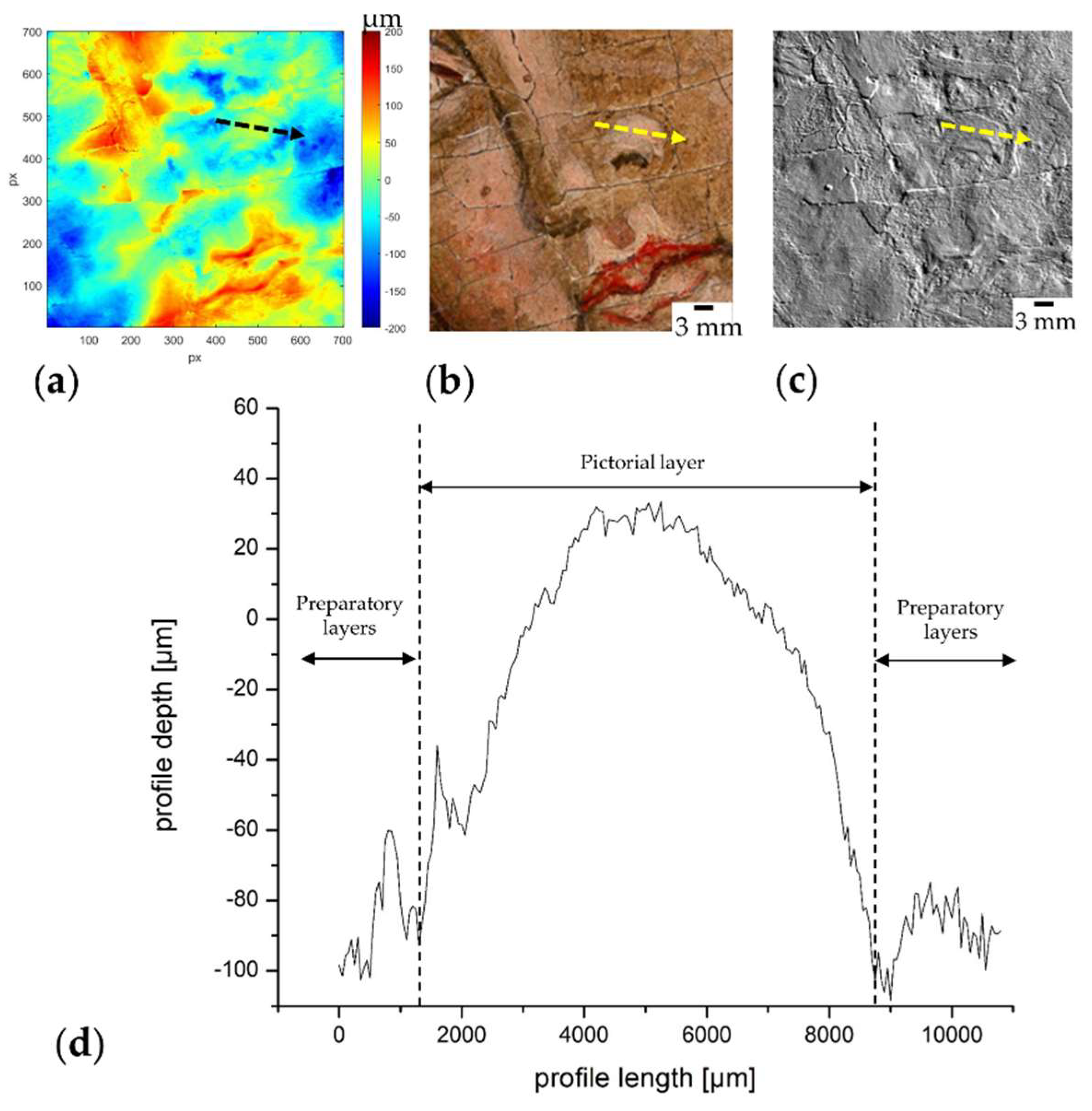
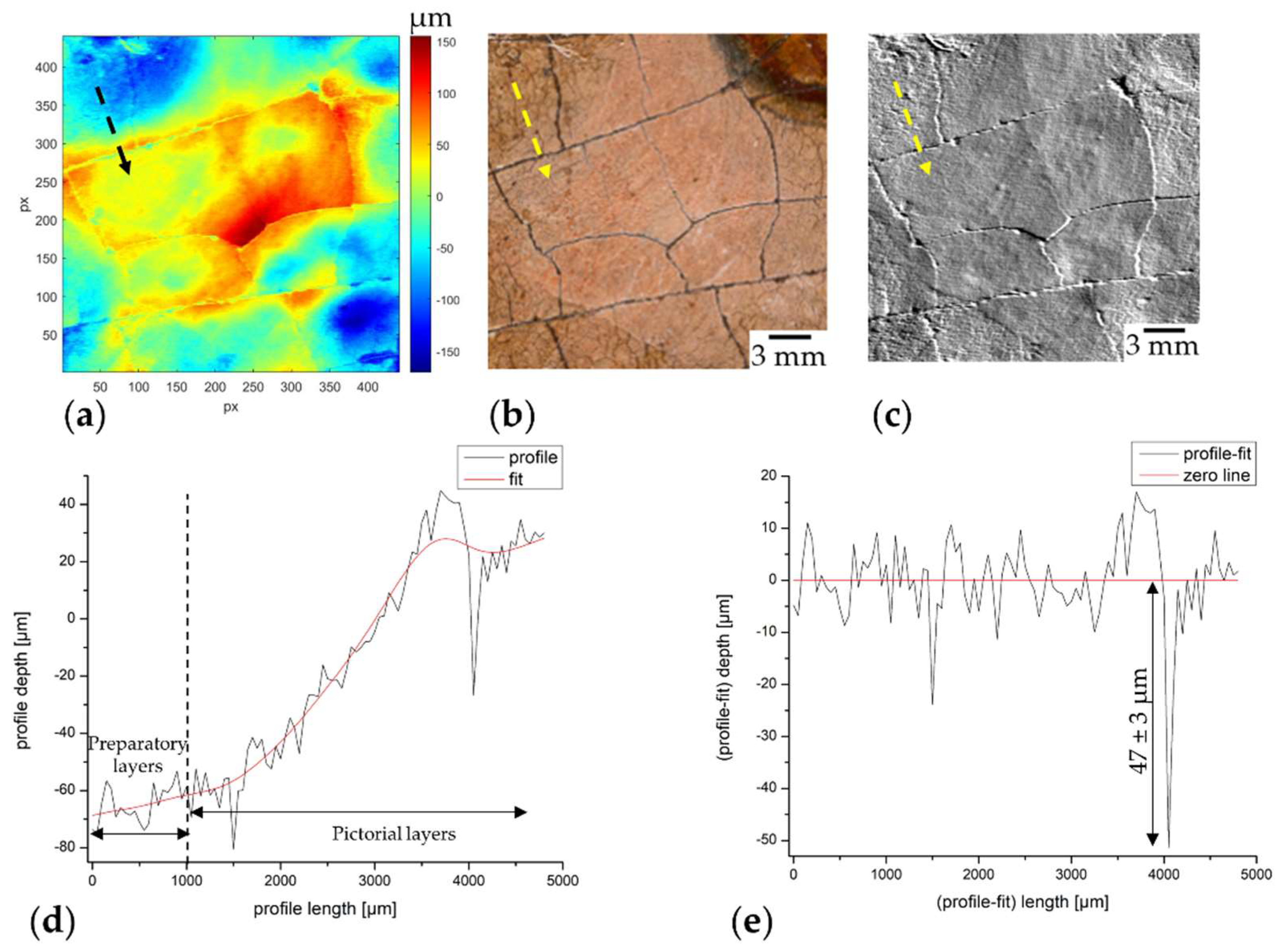
3.2. Study of the Artist’s Technique through Profilometric Data Processing

The micro-profilometry high-resolution 3D map allowed us to study the artist’s technique and obtain information on the conservation history of the painting. The map was elaborated with MATLAB to analyse brushstrokes and cracks.

In the simulated raking light image (Figure 5i), two surfaces with different morphological characteristics are discernible: the first one, corresponding to the flesh tone in Figure 5f, is very smooth, allowing for the visibility of the brushstrokes; the second one, corresponding to the green-brownish areas, appears grainy and irregular and is ascribable to the preparatory layer. The latter may have emerged during the 1970s restoration, when an alkaline solvent was used to remove the yellowed varnish [25], or may have been used as a green chromatic undertone left partially visible as the artist’s stylistic choice.

To corroborate the hypothesis that the green-brownish areas pertain to the preparatory layers, we measured the thickness of the brushstrokes across the grainy and smooth surfaces in several selected areas. For each area, we removed the shape by subtracting the best-fitting plane from the raw data to obtain the so-called conditioned surface where several profiles were then extracted. As an example, in Figure 6a, we report the results obtained on the Child’s nose. The black (Figure 6a) and yellow (Figure 6b,c) lines indicate the direction along which the profile has been extracted, which is reported in Figure 6d. The thickness of the brushstroke defining the naris was about 110 µm. For all selected areas, the brushstrokes stand above the grainy surface, supporting the hypothesis that the flesh tones were laid over the grainy surface, which can be attributed to the preparatory layers.

We analysed the cracks to investigate the succession in the application of the flesh tones to clarify whether they were original layers or later retouchings. We followed the same procedure described above, and the results obtained on the right Child’s cheek are shown in Figure 7.

To measure the depth of a crack, we extracted a profile along the dotted arrows in Figure 7a–c nine times. A smoothing spline function (red line in Figure 7d) was subtracted from the raw profiles, and the transition point from the preparatory to pictorial layer was obtained by calculating the inflection point of the spline function. The crack depth was measured with respect to the zero line in Figure 7e, resulting in being about 47 ± 3 µm. With the thickness of the flesh tone layer being in the order of 100 microns, the crack did not reach the preparatory layer.

We initially attributed the partial filling of the crack to the presence of pink pigment, supporting the hypothesis of successive repainting with the flesh tone. However, the simulated raking light image shows the continuity of the cracks across the scanned surface, with no interruptions between the preparatory layer and the flesh tones, suggesting that they cracked at the same time.

Raman spectra collected at several points on the pictorial surface proved the presence of the characteristic vibration peaks of aliphatic hydrocarbons [49] in the 2800–2900 cm⁻¹ region, ascribable to the presence of wax. Therefore, the wax was probably applied during the 1970s restoration to consolidate the pictorial layers. This operation was necessary given the tangential cut of the panel, which favours the warp with thermo-hygrometric condition variations. As the panel deformation often affects the intactness of the pictorial layers, restorers probably filled the cracks with wax to prevent paint-layer damage. Therefore, given the continuity of the cracks across the scanned area and the possibility that the cracks were filled with wax and not with the pink pigment, we hypothesise that the flesh tones are possibly coeval with the painting and not later retouchings.

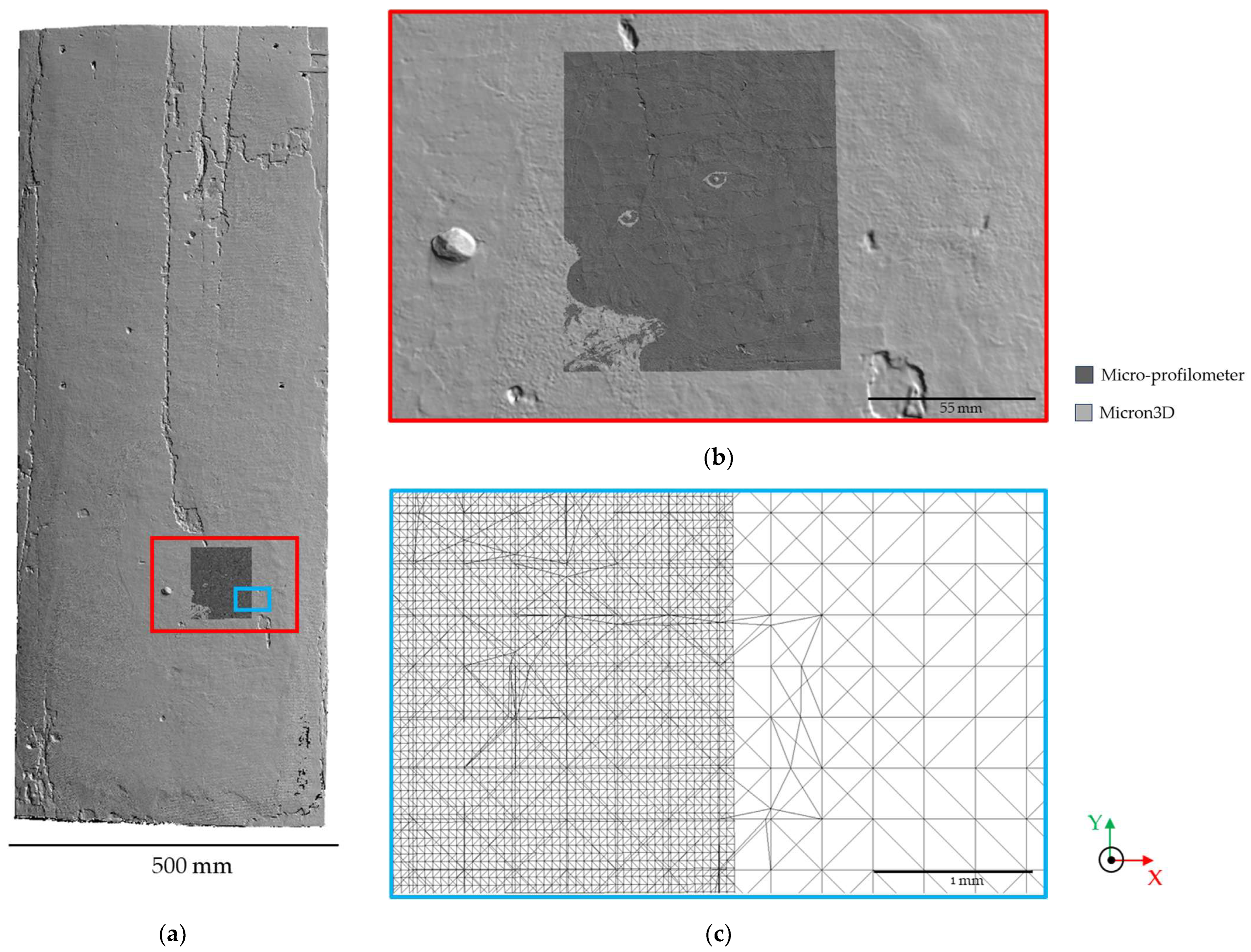
3.3. Multi-Scale and Multi-Resolution Fusion of 3D Data

We merged the post-restoration and micro-profilometric meshes using CloudCompare software (v.2.12.4) to obtain a multi-scale and multi-resolution 3D product. We aligned the models using two tools available in the software: first, the models were aligned manually using the Align (point pairs picking) tool by choosing homologous points on the meshes; then, the Iterative Closest Point (ICP) tool was applied for fine registration (final RMS 0.0263 mm). Finally, we merged (using the Merge tool) the aligned models into a single model (Figure 8).

The data fusion allowed us, on the one hand, to overcome the problem of missing points in the micro-profilometer mesh (black painted areas such as the Child’s eyes and the bottom-left corner, Figure 8b), and on the other hand, to increase the resolution of the post-restoration model in the region of the Child’s face (Figure 8c), enhancing the readability of the details.

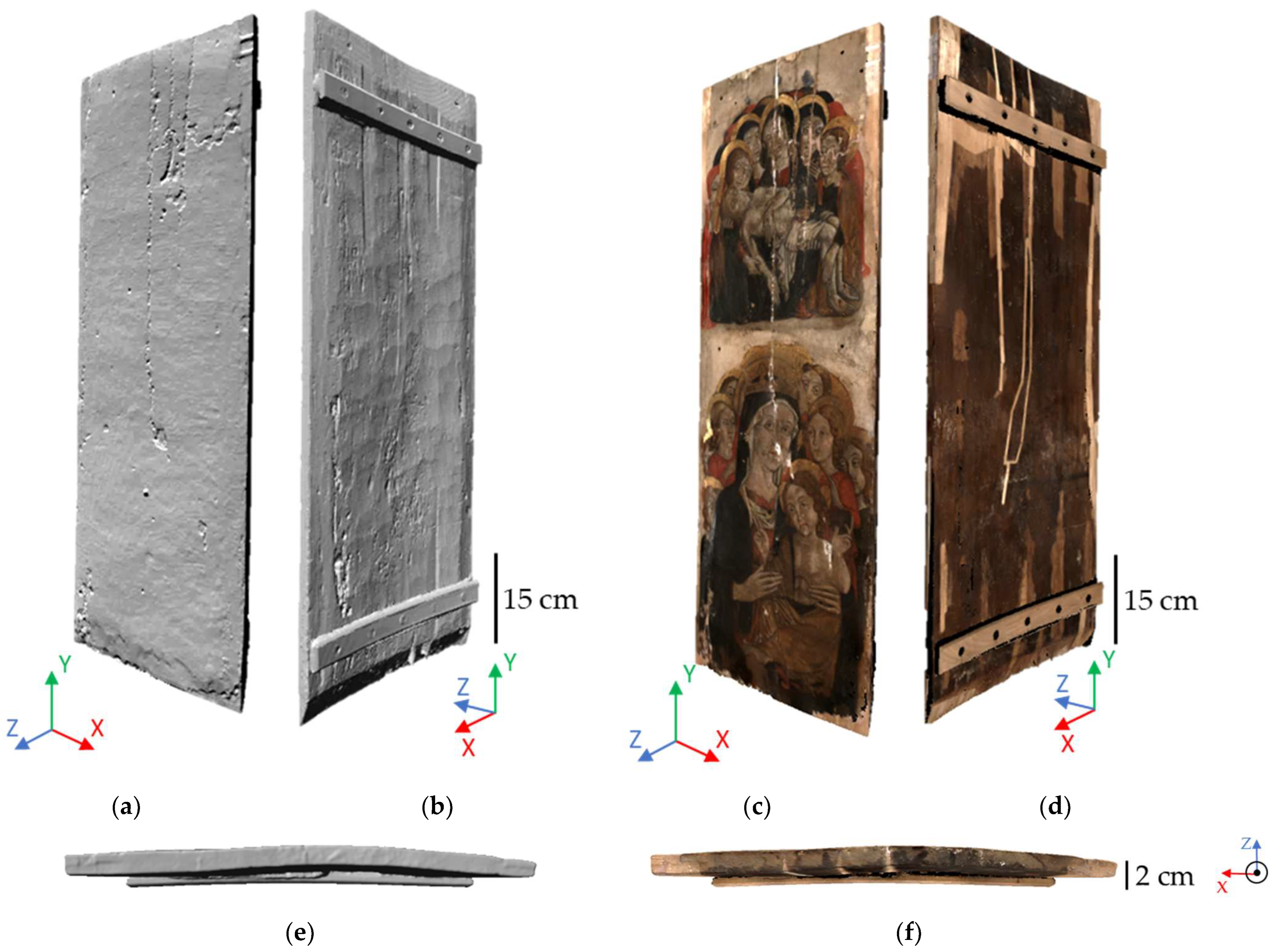
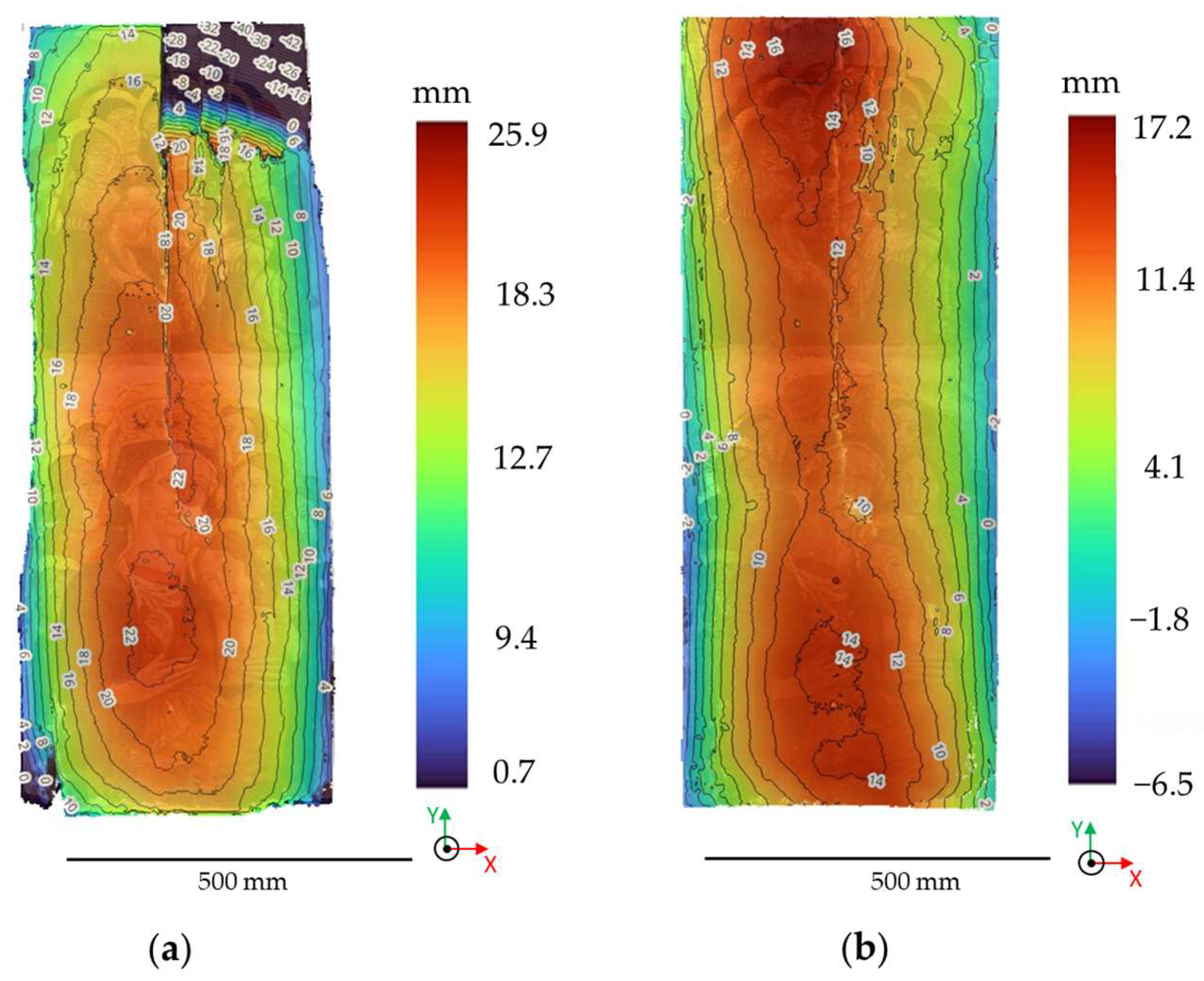
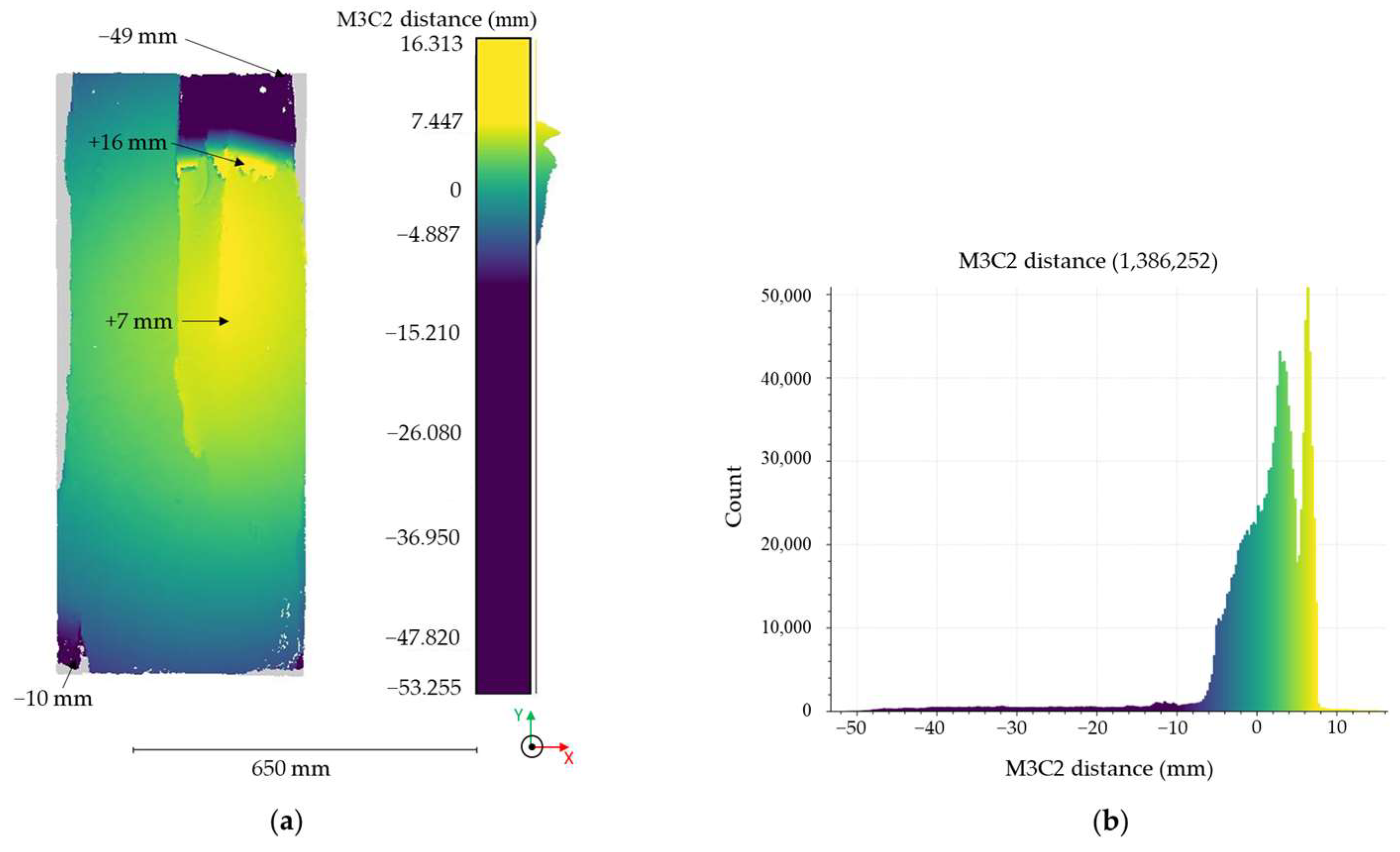
3.4. Three-Dimensional Data for Restoration Monitoring

One of the aims of this work was to document the shape variations due to restoration. To this end, we carried out a multi-temporal analysis between the pre- and post-restoration 3D models, obtained by close-range photogrammetry and structured-light topography, respectively. We used Digital Elevation Models (DEMs), the calculation of the warping arrow and the calculation of the distance between the two point clouds using the M3C2 (Multiscale Model to Model Cloud Comparison) algorithm.

A DEM is a raster image obtained by the projection of a point cloud onto a plane along the orthogonal direction. It is also known as a 2.5D model because it consists of a regular grid of pixels (XY), whose size is the DEM resolution, with altimetric information (Z) expressed in a colour scale [50]. We generated the Digital Elevation Models (0.14 Mpx, 1.97 mm/px resolution) from the dense point clouds using the open source CloudCompare software and imported them into QGIS software (v.3.34.5, https://www.qgis.org/it/site/, accessed on 12 December 2023), where contour lines (or isohypses, i.e., curves connecting points with the same elevation) were extracted with a 2 mm interval. Figure 9 shows the two DEMs, superimposed on the textured models, with the colour bars and contour lines.

In the pre-restoration DEM and isohypses (Figure 9a), the deflection of the panel and the almost complete detachment of the upper-right part are clearly visible and quantified by the contour lines. The post-restoration DEM (Figure 9b) documents the shape variations due to restoration. The warping of the panel in both the conservative states is clearly visible.

The warping arrow quantifies the deformation of the panel due to the placement of new crosspieces [51]. Since the arrow corresponds to the height of a circular segment, we calculated it by considering the section of the point cloud as a circumference, with an approximation valid for the lower panel surface due to the vertical fracture in the upper part of the pre-restoration model (Figure 3 and Figure 9a). Using CloudCompare software, we exported five cross-sections from the point clouds pre- and post-restoration every 6 cm (first column in

Table 3. Mean value and standard deviation of the warping arrows calculated on the point clouds.

		Mean Value ± St. Dev. [μm]
Post-Restoration Model with the Sections Where the Arrows Were Calculated Highlighted in Pink	Number of Section	Pre-Restoration Point Cloud	Post-Restoration Point Cloud
	1	18.3 ± 0.4	16.4 ± 0.4
	2	19.2 ± 0.1	16.7 ± 0.3
	3	18.7 ± 0.1	17.0 ± 0.3
	4	19.0 ± 0.1	16.6 ± 0.1
	5	18.5 ± 0.1	15.3 ± 0.5

), and we calculated the warping arrow nine times for each section. The mean value and the standard deviation are reported in Table 3, confirming the decrease in the panel warp after the consolidation of the wooden support.

We also calculated the point distances between the two clouds by applying the M3C2 algorithm [52] available in CloudCompare software. Other algorithms such as the C2C (simple nearest-neighbour Cloud-to-Cloud comparison) and C2M (Cloud-to-Mesh comparison) are available, but the M3C2 algorithm has proven to be well suited to handling complex geometries, accurate in estimating distance differences between two surfaces and robust to changes in point density and point cloud noise [53,54,55]. The M3C2 algorithm works directly on point clouds (without meshing) and computes the local distance between two clouds along the normal direction of the surface by creating a projection cylinder around each point of the reference cloud. The cylinder is projected back and forth from the point, and the distance from the nearest point in the cloud is given as a positive or negative value with respect to the reference cloud. For each distance, the algorithm estimates a confidence interval (limit of detection LOD95%), depending on the point cloud’s local roughness. The resulting model is displayed as a colour map, highlighting areas of elevation difference.

We aligned the two clouds using the Iterative Closest Point (ICP) algorithm. The M3C2 calculation was then started with the post-restoration cloud as the reference. Figure 10 shows the 3D rendering of the M3C2 algorithm with the relative colour bar indicating the recorded distance in the range of −53.3 mm to 16.3 mm. The colour bar was properly scaled to enhance the differences between the two clouds. Positive and negative values indicate areas that were lowered and raised along the z-axis, respectively. The largest height difference (−49 mm) was recorded in the upper-right part, where the panel was severely damaged by out-of-plane deformation, which was recovered with the restoration. In the central region, there was a shift of +7 mm between the right and left sides, which was flattened during the restoration.

4. Discussion and Conclusions

In this work, we applied close-range photogrammetry and structured-light topography to survey a panel painting before and after its restoration to document the repair intervention through a multi-temporal analysis of the conservation status. In addition, we performed a high-resolution 3D survey through micro-profilometry not only to obtain an in-depth insight into the artist’s technique, the history of the triptych and the previous restoration intervention, but also to evaluate the current state of conservation following the earthquake that severely damaged the painting.

Photogrammetry, used for the 3D modelling before restoration, did not allow the creation of a whole model of the panel due to the difficulty of acquiring the painting edges, which was solved in our previous work [29]. Therefore, the photogrammetric output consisted of two separate models, one for the front and the other one for the rear panel. After restoration, the whole painting was acquired with the structured-light scanner, and we realised the whole 3D model of the painting.

Notwithstanding the different instruments used for the painting survey before and after restoration, which is often the case when dealing with artwork conservation due to the very long lead times for the repair intervention, the rapid development of technology-based techniques and the turnover of research groups carrying out the measurements, we were able to carry out the multi-temporal analysis of the conservation status of the painting.

Furthermore, the pre-restoration model was used to plan the restoration intervention: the measurement of both the dramatic deformations of the support due to the earthquake and the cracks allowed us to properly design the panel repair. Moreover, the effect of the seismic event on the support influenced the conservative state of the pictorial layers, which was measured by micro-profilometry (paint detachments and micro-cracks).

The higher resolution of the post-restoration 3D model allowed the detection of pictorial details not visible in the photogrammetric model, such as contour drawings, brushstrokes and incisions. Although the scanner output consisted of a textured 3D model, the painting’s appearance was not faithful, being much darker than the original with undesired reflections in the gilded areas (Figure 4c). Conversely, the texture acquired with photogrammetry was very much in line with the real appearance of the painting, as expected (Figure 3d). The post-restoration model serves as a reference model for the future monitoring of the artwork: it will be the starting point for assessing the conservation of the painting and for evaluating any differences with subsequent restorations. It is likely that future surveys will be conducted with different instruments than those used in this work; therefore, the analysis carried out within this work is consistent with real cases.

The multi-temporal monitoring of the conservation status before and after restoration was helpful in documenting the effects of the complex and considerable consolidation of the wooden support. The main changes in the panel were the reduction in the warping arrow and the recovery of out-of-plane deformations and breaks, which were quantified and measured using the M3C2 algorithm.

The high-resolution mesh of the Child’s face by micro-profilometry disclosed a few issues about the artist’s technique, the history of the artwork and the previous restoration. It was possible to distinguish the preparatory layers from the pictorial ones, measure the thickness of the brushstrokes, analyse the craquelure, quantify the depth of the cracks and identify the effects of the previous restoration, e.g., the presence of wax used to consolidate the pictorial layers.

The high resolution of micro-profilometry made this technique well suited for studying the micro-deformations in the pictorial layers, while photogrammetry and structured-light topography were more appropriate for the analysis of macro-deformations in the support. The integration and merging of the results from different 3D techniques was of added value in the study of the panels, allowing for an exhaustive analysis both at the micro and macro level.

Our future goal is the digitisation of the panel depicting St Michael the Archangel to complete the 3D acquisition of the triptych.

References

1. Arbace, L.; Sonnino, E.; Callieri, M.; Dellepiane, M.; Fabbri, M.; Idelson, A.I.; Scopigno, R. Innovative Uses of 3D Digital Technologies to Assist the Restoration of a Fragmented Terracotta Statue. J. Cult. Heritage 2013, 14, 332–345. [Google Scholar] [CrossRef]
2. Pieraccini, M.; Guidi, G.; Atzeni, C. 3D Digitizing of Cultural Heritage. J. Cult. Heritage 2001, 2, 63–70. [Google Scholar] [CrossRef]
3. Gabellone, F. Digital Twin: A New Perspective for Cultural Heritage Management and Fruition. Acta IMEKO 2022, 11, 7. [Google Scholar] [CrossRef]
4. Apollonio, F.I.; Basilissi, V.; Callieri, M.; Dellepiane, M.; Gaiani, M.; Ponchio, F.; Rizzo, F.; Rubino, A.R.; Scopigno, R.; Sobra’, G. A 3D-Centered Information System for the Documentation of a Complex Restoration Intervention. J. Cult. Heritage 2018, 29, 89–99. [Google Scholar] [CrossRef]
5. Robson, S.; Bucklow, S.; Woodhouse, N.; Papadaki, H. Periodic Photogrammetric Monitoring and Surface Reconstruction of a Historical Wood Panel Painting for Restoration Purposes. Int. Arch. Photogramm. Remote Sens. Spat. Inf. Sci. 2004, 35, 395–400. [Google Scholar]
6. Bratasz, L.; Jakiela, S.; Kozlowski, R. Allowable Thresholds in Dynamic Changes of Microclimate for Wooden Cultural Objects: Monitoring in Situ and Modelling. In Proceedings of the ICOM Committee for Conservation, 14th Triennial Meeting, The Hague, The Netherlands, 12–16 September 2005; pp. 582–589. [Google Scholar]
7. Guidi, G.; Beraldin, J.-A.; Atzeni, C. Wood artworks dimensional monitoring through high-resolution 3D cameras. Proc. SPIE 2007, 6491, 64910T. [Google Scholar] [CrossRef]
8. Hess, M.; Korenberg, C.; Ward, C.; Robson, S.; Entwistle, C. Use of 3D Laser Scanning for Monitoring the Dimensional Stability of a Byzantine Ivory Panel. Stud. Conserv. 2015, 60, S126–S133. [Google Scholar] [CrossRef]
9. Palma, G.; Pingi, P.; Siotto, E.; Bellucci, R.; Guidi, G.; Scopigno, R. Deformation Analysis of Leonardo da Vinci’s “Adorazione dei Magi” through Temporal Unrelated 3D Digitization. J. Cult. Heritage 2019, 38, 174–185. [Google Scholar] [CrossRef]
10. Guidi, G.; Atzeni, C.; Seracini, M.; Lazzari, S. Painting Survey by 3D Optical Scanning: The Case of “Adoration of the Magi” by Leonardo Da Vinci. Stud. Conserv. 2004, 49, 1–12. [Google Scholar] [CrossRef]
11. Baribeau, R.; Rioux, M.; Godin, G. Recent Advances in the Use of a Laser Scanner in the Examination of Paintings. In Proceedings of the Restoration ’92 Conference, Amsterdam, The Netherlands, 20–22 October 1992. [Google Scholar]
12. Bertani, D.; Cetica, M.; Melozzi, M.; Pezzati, L. High-Resolution Optical Topography Applied to Ancient Painting Diagnostics. Opt. Eng. 1995, 34, 1219–1225. [Google Scholar] [CrossRef]
13. Brewer, A.; Forno, C. Moiré Fringe Analysis of Cradled Panel Paintings. Stud. Conserv. 1997, 42, 211–230. [Google Scholar] [CrossRef]
14. Abate, D.; Menna, F.; Remondino, F.; Gattari, M. 3D Painting Documentation: Evaluation of Conservation Conditions with 3D Imaging and Ranging Techniques. Int. Arch. Photogramm. Remote. Sens. Spat. Inf. Sci. 2014, XL-5, 1–8. [Google Scholar] [CrossRef]
15. Targowski, P.; Iwanicka, M. Optical Coherence Tomography: Its Role in the Non-Invasive Structural Examination and Conservation of Cultural Heritage Objects—A Review. Appl. Phys. A 2012, 106, 265–277. [Google Scholar] [CrossRef]
16. Daffara, C.; Mazzocato, S. Surface Metrology Based on Scanning Conoscopic Holography for In Situ and In-Process Monitoring of Microtexture in Paintings. Sensors 2022, 22, 6637. [Google Scholar] [CrossRef]
17. Ramos, M.M.; Remondino, F. Data fusion in Cultural Heritage—A Review. Int. Arch. Photogramm. Remote. Sens. Spat. Inf. Sci. 2015, XL-5/W7, 359–363. [Google Scholar] [CrossRef]
18. Gašparović, M.; Malarić, I. Increase of readability and accuracy of 3D models using fusion of close range photogrammetry and laser scanning. Int. Arch. Photogramm. Remote. Sens. Spat. Inf. Sci. 2012, XXXIX–B5, 93–98. [Google Scholar] [CrossRef]
19. Fontana, R.; Gambino, M.C.; Greco, M.; Marras, L.; Materazzi, M.; Pampaloni, E.; Pezzati, L.; Poggi, P. Integrating 2D and 3D Data for Diagnostics of Panel Paintings. Proc. SPIE 2003, 5146, 88–98. [Google Scholar] [CrossRef]
20. Grifoni, E.; Legnaioli, S.; Nieri, P.; Campanella, B.; Lorenzetti, G.; Pagnotta, S.; Poggialini, F.; Palleschi, V. Construction and Comparison of 3D Multi-Source Multi-Band Models for Cultural Heritage Applications. J. Cult. Heritage 2018, 34, 261–267. [Google Scholar] [CrossRef]
21. Chane, C.S.; Mansouri, A.; Marzani, F.S.; Boochs, F. Integration of 3D and Multispectral Data for Cultural Heritage Applications: Survey and Perspectives. Image Vis. Comput. 2013, 31, 91–102. [Google Scholar] [CrossRef]
22. Fontana, R.; Gambino, M.C.; Greco, M.; Marras, L.; Materazzi, M.; Pampaloni, E.; Pelagotti, A.; Pezzati, L.; Poggi, P.; Sanapo, C. 2D and 3D Optical Diagnostic Techniques Applied to Madonna Dei Fusi by Leonardo Da Vinci. Proc. SPIE 2005, 5857, 166–176. [Google Scholar] [CrossRef]
23. Guarnieri, A.; Remondino, F.; Vettore, A. Digital Photogrammetry and TLS Data Fusion Applied to Cultural Heritage 3D Modeling. Int. Arch. Photogramm. Remote Sens. Spat. Inf. Sci. 2006, 36, 1–6. [Google Scholar]
24. Bastonero, P.; Donadio, E.; Chiabrando, F.; Spanò, A. Fusion of 3D Models Derived from TLS and Image-Based Techniques for CH Enhanced Documentation. ISPRS Ann. Photogramm. Remote. Sens. Spat. Inf. Sci. 2014, II–5, 73–80. [Google Scholar] [CrossRef]
25. AA. VV. Restauri nelle Marche. Testimonianze Acquisti e Recuperi; Arti Grafiche Editoriali: Urbino, Italia, 1973. [Google Scholar]
26. Barucca, G. Galleria Degli Uffizi Facciamo Presto! Marche 2016–2017: Tesori Salvati, Tesori Da Salvare; Prima Edizione; Giunti Firenze Musei: Firenze, Italy, 2017; ISBN 978-88-09-85696-7. [Google Scholar]
27. Campbell, J.B.; Wynne, R.H.; Thomas, V.A. Introduction to Remote Sensing, 6th ed.; The Guilford Press: New York, NY, USA, 2023; ISBN 978-1-4625-4940-5. [Google Scholar]
28. Linder, W. Digital Photogrammetry: Theory and Applications; Springer: Berlin/Heidelberg, 2013; ISBN 978-3-662-06725-3. [Google Scholar]
29. Grifoni, E.; Vannini, E.; Lunghi, I.; Faraioli, P.; Ginanni, M.; Santacesarea, A.; Fontana, R. 3D Multi-Modal Point Clouds data Fusion for Metrological Analysis and Restoration Assessment of a Panel Painting. J. Cult. Heritage 2024, 66, 356–366. [Google Scholar] [CrossRef]
30. Lehoczky, M.; Abdurakhmonov, Z. Present Software of Photogrammetric Processing of Digital Images. E3S Web Conf. 2021, 227, 04001. [Google Scholar] [CrossRef]
31. Remondino, F.; Nocerino, E.; Toschi, I.; Menna, F. A Critical review of automated photogrammetric processing of large datasets. Int. Arch. Photogramm. Remote Sens. Spat. Inf. Sci. 2017, XLII–2/W5, 591–599. [Google Scholar] [CrossRef]
32. Lavecchia, F.; Guerra, M.G.; Galantucci, L.M. Performance Verification of a Photogrammetric Scanning System for Micro-Parts Using a Three-Dimensional Artifact: Adjustment and Calibration. Int. J. Adv. Manuf. Technol. 2018, 96, 4267–4279. [Google Scholar] [CrossRef]
33. Luhmann, T.; Robson, S.; Kyle, S. Close-Range Photogrammetry: Principles, Methods and Applications; Whittles: Dunbeath, UK, 2006; ISBN 978-1-870325-50-9. [Google Scholar]
34. Bertin, S.; Friedrich, H.; Delmas, P.; Chan, E.; Gimel’farb, G. Digital Stereo Photogrammetry for Grain-Scale Monitoring of Fluvial Surfaces: Error Evaluation and Workflow Optimisation. ISPRS J. Photogramm. Remote. Sens. 2015, 101, 193–208. [Google Scholar] [CrossRef]
35. Remondino, F.; El-Hakim, S. Image-based 3D Modelling: A Review. Photogramm. Rec. 2006, 21, 269–291. [Google Scholar] [CrossRef]
36. Remondino, F.; Rizzi, A.; Barazzetti, L.; Scaioni, M.; Fassi, F.; Brumana, R.; Pelagotti, A. Review of Geometric and Radiometric Analyses of Paintings. Photogramm. Rec. 2011, 26, 439–461. [Google Scholar] [CrossRef]
37. Brutto, M.L.; Garraffa, A.; Pellegrino, L.; Di Natale, B. 3D Mosaic Documentation Using Close Range Photogrammetry. In Proceedings of the 1st International Conference on Metrology for Archaeology, Benevento, Italy, 21–23 October 2015; pp. 22–23. [Google Scholar]
38. Luhmann, T.; Robson, S.; Kyle, S.; Boehm, J. Close-Range Photogrammetry and 3D Imaging; De Gruyter: Berlin, Germany, 2019; ISBN 978-3-11-060725-3. [Google Scholar]
39. Bell, T.; Li, B.; Zhang, S. Structured Light Techniques and Applications. In Wiley Encyclopedia of Electrical and Electronics Engineering; Webster, J.G., Ed.; Wiley: Hoboken, NJ, USA, 2016; pp. 1–24. ISBN 978-0-471-34608-1. [Google Scholar]
40. Akca, D.; Remondino, F.; Novák, D.; Hanusch, T.; Schrotter, G.; Gruen, A. Performance evaluation of a coded structured light system for cultural heritage applications. Proc. SPIE 2007, 6491, 64910V. [Google Scholar] [CrossRef]
41. Fontana, R.; Gambino, M.C.; Mazzotta, C.; Greco, M.; Pampaloni, E.; Pezzati, L. High-Resolution 3D Survey of Artworks. Proc. SPIE 2004, 5457, 719–726. [Google Scholar] [CrossRef]
42. Carcagni, P.; Daffara, C.; Fontana, R.; Gambino, M.C.; Mastroianni, M.; Mazzotta, C.; Pampaloni, E.; Pezzati, L. Optical Micro-Profilometry for Archaeology. Proc. SPIE 2005, 5857, 58570F. [Google Scholar] [CrossRef]
43. Daffara, C.; Mazzocato, S.; Marchioro, G. Multiscale Roughness Analysis by Microprofilometry Based on Conoscopic Holography: A New Tool for Treatment Monitoring in Highly Reflective Metal Artworks. Eur. Phys. J. Plus 2022, 137, 430. [Google Scholar] [CrossRef]
44. Mazzocato, S.; Cimino, D.; Daffara, C. Integrated Microprofilometry and Multispectral Imaging for Full-Field Analysis of Ancient Manuscripts. J. Cult. Heritage 2024, 66, 110–116. [Google Scholar] [CrossRef]
45. Fovo, A.D.; Striova, J.; Pampaloni, E.; Fontana, R. Unveiling the Invisible in Uffizi Gallery’s Drawing 8P by Leonardo with Non-Invasive Optical Techniques. Appl. Sci. 2021, 11, 7995. [Google Scholar] [CrossRef]
46. Pamart, A.; Abergel, V.; de Luca, L.; Veron, P. Toward a Data Fusion Index for the Assessment and Enhancement of 3D Multimodal Reconstruction of Built Cultural Heritage. Remote. Sens. 2023, 15, 2408. [Google Scholar] [CrossRef]
47. Moyano, J.; Nieto-Julián, J.E.; Bienvenido-Huertas, D.; Marín-García, D. Validation of Close-Range Photogrammetry for Architectural and Archaeological Heritage: Analysis of Point Density and 3D Mesh Geometry. Remote Sens. 2020, 12, 3571. [Google Scholar] [CrossRef]
48. Kodors, S. Point Distribution as True Quality of LiDAR Point Cloud. Balt. J. Mod. Comput. 2017, 5, 362–378. [Google Scholar] [CrossRef]
49. Burgio, L.; Clark, R.J. Library of FT-Raman Spectra of Pigments, Minerals, Pigment Media and Varnishes, and Supplement to Existing Library of Raman Spectra of Pigments with Visible Excitation. Spectrochim. Acta Part A Mol. Biomol. Spectrosc. 2001, 57, 1491–1521. [Google Scholar] [CrossRef] [PubMed]
50. Riminesi, C.; Del Fà, R.M.; Brizzi, S.; Rocco, A.; Fontana, R.; Bertasa, M.; Grifoni, E.; Impallaria, A.; Leucci, G.; De Giorgi, L.; et al. Architectural Assessment of Wall Paintings Using a Multimodal and Multi-Resolution Diagnostic Approach: The Test Site of the Brancacci Chapel in Firenze. J. Cult. Heritage 2024, 66, 99–109. [Google Scholar] [CrossRef]
51. Cocchi, L.; Bertrand, M.; Mazzanti, P.; Uzielli, L.; Castelli, C.; Santacesaria, A. Verfica Del Funzionamento Di Una Traversatura Elastica Applicata Su Un Dipinto Su Tavola: La Deposizione Dalla Croce Di Anonimo Abruzzese, XVI Secolo. OPD Restauro 2014, 26, 83–94. Available online: https://www.jstor.org/stable/24398164 (accessed on 13 January 2024).
52. Lague, D.; Brodu, N.; Leroux, J. Accurate 3D Comparison of Complex Topography with Terrestrial Laser Scanner: Application to the Rangitikei Canyon (N-Z). ISPRS J. Photogramm. Remote Sens. 2013, 82, 10–26. [Google Scholar] [CrossRef]
53. Rose, W.; Bedford, J.; Howe, E.; Tringham, S. Trialling an Accessible Non-Contact Photogrammetric Monitoring Technique to Detect 3D Change on Wall Paintings. Stud. Conserv. 2022, 67, 545–555. [Google Scholar] [CrossRef]
54. La Rocca, A.; Lingua, A.M.; Grigillio, D. A photogrammetry application to rockfall monitoring: The Belca, Slovenia case study. GEAM 2020, 1208, 16–33. [Google Scholar] [CrossRef]
55. Nourbakhshbeidokhti, S.; Kinoshita, A.M.; Chin, A.; Florsheim, J.L. A Workflow to Estimate Topographic and Volumetric Changes and Errors in Channel Sedimentation after Disturbance. Remote. Sens. 2019, 11, 586. [Google Scholar] [CrossRef]
Figure 1. The Nocria triptych (a) before and (b) after the earthquake.
Heritage 07 00103 g001
Figure 2. (a) Photogrammetry set-up: shooting distance D1 = 115 cm and baseline B = 20.7 cm; (b) structured-light set-up: working distance D2 = 70 cm.
Heritage 07 00103 g002
Figure 3. Products of the photogrammetric survey of the front of the panel before the restoration: (a) sparse cloud; (b) dense cloud; (c) mesh visualised with simulated raking light; (d) textured model.
Heritage 07 00103 g003
Figure 4. Three-dimensional mesh created after restoration with the Micron3D scanner: (a) front and (b) back view with simulated raking light; (c) front and (d) back view of the textured model; top view of the (e) mesh and (f) textured model.
Heritage 07 00103 g004
Figure 5. Back view of the (a) pre- and (b) post-restoration models with wooden inserts highlighted by two yellow arrows. (c) Visible image of the front of the panel with the areas of the halo and the Child’s face highlighted in yellow and blue, respectively. Halo’s (d) visible image and (e) 3D model (Micron3D). Child’s face’s (f) visible image and 3D model (g), pre-restoration (photogrammetry) and (h) post-restoration by structured-light and (i) micro-profilometry.
Heritage 07 00103 g005
Figure 6. Detail of the Child’s face: (a) conditioned surface; (b) visible and (c) simulated raking light image. The dotted arrow in (ac) indicates the direction of the profile shown in (d).
Heritage 07 00103 g006
Figure 7. Detail of the Child’s right cheek: (a) conditioned surface; (b) visible and (c) simulated raking light image. The dotted arrow in (ac) indicates the direction along which we extracted the profile plotted in (d) (black line) with the spline function (red line); (e) profile after the subtraction of the shape to measure the depth of the crack.
Heritage 07 00103 g007
Figure 8. (a) Post-restoration and micro-profilometric 3D mesh merged in a single model; details of the Child’s face (b) in raking light and (c) in wireframe modality to highlight the different model resolutions.
Heritage 07 00103 g008
Figure 9. (a) Pre- and (b) post-restoration DEMs and contour lines obtained from the point clouds.
Heritage 07 00103 g009
Figure 10. (a) M3C2 rendering with the most significant distances. The integrations, present only in the post-restoration model, are displayed in grey as the software could not find a match; (b) histogram of the distribution of the computed distances.
Heritage 07 00103 g010