Using Explainable Artificial Intelligence (XAI) to Predict the Influence of Weather on the Thermal Soaring Capabilities of Sailplanes for Smart City Applications

Abstract

Background: Drones, also known as unmanned aerial vehicles, could potentially be a key part of future smart cities by aiding traffic management, infrastructure inspection and maybe even last mile delivery. This paper contributes to the research on managing a fleet of soaring aircraft by gaining an understanding of the influence of the weather on soaring capabilities. To do so, machine learning algorithms were trained on flight data, which was recorded in the UK over the past ten years at selected gliding clubs (i.e., sailplanes). Methods: A random forest regressor was trained to predict the flight duration and a random forest (RF) classifier was used to predict whether at least one flight on a given day managed to soar in thermals. SHAP (SHapley Additive exPlanations), a form of explainable artificial intelligence (AI), was used to understand the predictions given by the models. Results: The best RF have a mean absolute error of 5.7 min (flight duration) and an accuracy of 81.2% (probability of soaring in a thermal on a given day). The explanations derived from SHAP are in line with the common knowledge about the effect of weather systems to predict soaring potential. However, the key conclusion of this study is the importance of combining human knowledge with machine learning to devise a holistic explanation of a machine learning model and to avoid misinterpretations.

1. Introduction

Methods of soaring have generated intense interest and investigation since the earliest attempts at human flight [1]. The ability of larger birds, like the albatross, golden eagle and the red kite, to extract energy from the relative movement of air masses in both vertical and horizontal flight, without seemingly a flap of their wings, has received increasing interest since the early 20th century [1,2]. This observation is especially relevant for the flight patterns of larger birds, where ‘flapping flight’ would be unsustainable, due to the increased energy expenditure [1]. Emulating this skill is the goal of glider pilots, in their quest to stay airborne for as long as possible.

In general, soaring can be categorised into two distinct types of flight, known as static soaring and dynamic soaring [3]. Static soaring is flight conducted in rising air, which is commonly used by glider pilots. The choices available include the ability to fly in thermals, generated by pockets of rising air, or to transit back and forth along a ridge to use the vertical component of the wind blowing against the elevation (i.e., orographic lift, ridge flying) [3]. Dynamic soaring is harvesting energy from flying through wind gradients. It is a common sight in nature used by seabird populations, like petrels, who fly over the Southern and Pacific oceans while rarely flapping their wings [4].

The focus of this study is soaring in land-generated thermals, a commonly used technique in gliding circles to enable pilots who wish to remain airborne [3]. Thermals are created by a mass of air rising due to changes in temperature or humidity, in relation to the other surrounding air, and in close proximity to the ground [3]. This parcel of warm air rises due to its lower mass density forming a ‘thermal bubble’ [5]. At ground level, if the air is homogeneously heated-up or contains the same moisture level, an equilibrium exists. Therefore, it will not begin to rise (trigger), as no air is rushing in to take its place [6]. The air will only rise when an instability occurs (e.g., a non-homogeneous ground surface, non-homogeneous heating or air turbulence) [6]. The fact that thermals depend on instability, have a limited lifespan and drift in the wind makes them difficult to predict with any level of certainty [6]. Furthermore, thermals are transparent and there is, as of 2019, no reliable way to measure this rising air apart from flying through it [6].

With the increase in interest in drones, also known as unmanned aerial vehicles (UAVs), research into soaring flight is gaining rapid momentum. While progress has been made on energy storage systems for UAVs, it is still a limiting factor for their operational use [2]. Therefore, research interests are once again pointing towards the merits of engineless flight to extend flight durations [2].

UAVs have undergone significant development in that past decade [7]. Industries are trialling this emerging technology in more and more diverse applications [8]. They can offer substantial cost saving in agriculture through crop condition monitoring [7], weed detection [9], irrigation scheduling [10] and pesticide spraying for precision agriculture [11]. UAVs can also support pasture management to optimise the rotation of grazing for cattle [12]. They can aid in disaster management by surveying difficult-to-reach locations post-event [13]. They can help firefighters to correctly manage wildfires [14]. They are especially pertinent in flood detection and monitoring [15], as UAVs are more capable of providing the necessary aerial images than their satellite counterparts [16]. Also, in the realm of ecological preservation, UAVs can capture greater detail than satellites, allowing ecologists and authorities to monitor the effect of tourism (e.g., ‘trampling’) in nature areas [17] or litter on beaches [18]. In the construction industry, UAVs support tasks including the surveying of earthworks, aspects of site management, progress monitoring, safety inspection and damage assessment [19]. UAVs are a key player and a leading technology in the development of smart cities [20,21]. They can aid traffic monitoring and infrastructure inspections of roads, bridges, and power lines, as well as urban parcel and freight delivery [20]. They can provide entertainment and advertising services, as well as security alarms [21]. It should be noted that not all researchers and stakeholders agree on whether UAVs are suitable choices for deliveries in the urban environment [22].

The flight duration, or battery life of UAVs, is listed as a major shortcoming in various applications [6,7,11,23], and it results in the requirement of complicated battery swapping and recharging procedures [21]. To prolong the flight duration by enabling UAVs to soar (i.e., extracting energy from the environment) has been suggested as a solution [6,13,24]. This could further reduce the energy requirement of UAVs [25] and, therefore, contribute to the aim of net zero emissions. As the flight time of UAVs is not restricted by human endurance, soaring UAVs would be able to stay airborne for longer periods [24].

An inherent disadvantage of sailplane soaring is that the glider must adjust their flight path to incorporate thermals or fly along a ridge to gain a higher altitude before continuing their journey [6]. Therefore, soaring may not be the most suitable way to gain altitude for drones with time-sensitive deliveries. However, during competitions, pilots can reach average speeds exceeding 135 km/h over 750 km lengths, with the highest performing gliders (https://www.fai.org/news/looking-forward-2023-gliding-competition-season, accessed on 11 October 2023). Also, many proposed application areas are not as time-sensitive but require extensive flight times such as constant wildfire monitoring [14], environmental monitoring [26] and general surveillance [23]. Therefore, the issue of flight interruptions to enable soaring would not be a dramatic issue and could be solved by using a fleet of UAVs.

This paper contributes to the research on managing a fleet of soaring aircraft by gaining an understanding of the potential influence of weather on soaring capabilities. To do so, machine learning algorithms have been trained on past sailplane flight data. Generating the required flight data using autonomously soaring UAVs would be financially prohibitive. However, the logbook data of glider pilots are plentiful and provide a low-cost alternative for data acquisition. In short, the research provides a learning opportunity regarding the operation of soaring UAVs and provides a valuable insight on how weather and operational constraints influence the soaring capabilities of sailplanes to improve the efficiency and time management of gliding sites. Furthermore, this study also highlights the importance of combining human knowledge with explainable AI, to avoid misinterpretation.

2. Literature Review

The published literature available on gliding site optimisation is understandably rather limited. The influence of weather on the operational management of a soaring UAV fleet is also lacking in the public domain. Papers have been published investigating the use of soaring in thermals to extend the flight of UAVs [3]. Over the last decade, various researchers have addressed the challenges of autonomously centring in thermals, predicting the best flight path through simulated updrafts, and more recently, autonomously identifying where the thermals may be located in simulated environments. The tools and algorithms have been developed for UAVs and/or competition glider pilots.

2.1. Soaring Gliders and Unmanned Aerial Vehicles

While the dynamics of soaring flights are well understood by humans, programming the control laws to soar in unforeseen wind gradients and updrafts remained a challenge in 2019 [4]. The location and strengths of rising air are generally random and difficult to predict [6], because the shape, strength and location of thermals are influenced by complex atmospheric conditions, as well as the time of day, season of the year, and the undulation of the ground [6]. Examples of research on this topic include Dickmanns [27], who focused on competition soaring to determine the best cross-country trajectory arcs. However, they acknowledged that these results are only theoretical upper limits, which will not be easily achievable in the real world, due to a lack of knowledge about thermal activity. Chudej et al. [5] created a numerical model of thermal updrafts and implemented these into the three-dimensional equations of motion. Lee et al. [24] developed an autonomous soaring controller for an unpowered UAV and applied it in a simulated environment with multiple thermals. Schermann et al. [6] proposed a stochastic optimisation problem with the goal to optimise the flight trajectory through thermals for UAVs. Their control algorithm suggests when the glider should climb in a thermal, depending on its strength, and when it should ignore that thermal and continue to fly the track at a specific speed.

Heuristics (as in [24]) are a commonly used technique to find the location and strengths of thermals [25]. It is an obvious choice, owing to the uncertainty of the updraft and its strengths; making it difficult to formalise [25]. As the velocity of the rising air tends to be strongest in the centre of a thermal [6], early research therefore focused on methods to centre gliders in these thermals [24]. In fact, most of the research until 2012 was focused on utilising thermals efficiently, as opposed to finding them [28]. Thanks to the increasing computational power of onboard computers, several autonomous soaring algorithms have been proposed and developed [6]. Some initial research has been undertaken on finding thermals; for example, Cui et al. [28] used reinforcement learning to develop an ‘area exploring strategy’ to seek and benefit from thermal updrafts. They tested their strategy in a simulated environment with random thermals.

Applying the principles of ridge soaring in an urban environment, White et al. [3] conducted a feasibility study of micro air vehicles (MAVs) soaring next to tall buildings. Using a scale model of a building in a wind tunnel, they measured the vertical wind velocity component and concluded that this is lower than the sink rate of their experimental MAV. This indicates that soaring in the updraft next to tall buildings may be possible, in a similar fashion to conventional ridge soaring. On the operational side of things, Camacho et al. [25] proposed an architecture for the autonomous soaring of a swarm of cooperative autonomous gliders, with a goal of maximising the cumulative energy capture. Coutinho et al. [13] proposed a glider routing and trajectory optimisation problem (GRTOP) to find the best combinations of routes and trajectories for a fleet of UAVs, for use in disaster management [13]. However, they only used the ‘equations of motion’ for dynamic soaring. Dynamic soaring is of clearly more interest in the academic literature, compared to other forms of soaring, for UAVs [4]. In contrast, this paper adds to the research on thermal soaring, as the focus is on soaring UAVs in urban and rural environments over land. The required wind gradients for dynamic soaring are rather uncommon over land, as they are mainly found offshore close to the water surface [29], and this reduces the applicability of such a soaring technique over land [29]. Also, the flight trajectory required for dynamic soaring may be unsuitable for flight within cities [3]. As the long-term goal of this research is to create soaring UAVs for application in rural or urban environments, this study focuses on thermal soaring.

2.2. Contribution

This paper clearly differs from past research as it is not focussed on the actual process of soaring. The focus of this study is on using explainable AI to gain an understanding of how weather and operational constraints influence the soaring capabilities of aircrafts. This study uses a real-world dataset, that has not been collected in a controlled environment, to train a neural network (NN). The use of flight data from controlled experiments would not always be applicable to the real-world situation of a gliding club. It is entirely possible that the average flying duration is shorter on the best soaring days due to so many people being there, and, therefore, the flight duration being restricted, in order to allow everyone to fly the same glider. And, during hot weather, the efficiency of humans launching gliders and pulling them back to the start point after landing may be reduced. On less thermic days, it may be more of a struggle to stay airborne, but without additional demand for the glider, flight durations of multiple hours are also possible. The same can happen to soaring UAVs; their operational task may affect their ability to soar in thermals and therefore they are not just weather-dependent. By using real data, this study considers these factors.

Understanding the influence of weather on soaring capabilities is key to UAV operators. On days where there is not enough thermal activity, the operator must rely on battery swapping or charging. On days with marginal weather, the operator may need to deploy many drones to allow for sufficient time to thermal. Only a few drones are necessary on great soaring days with quicker height gains. Given that explainability is considered a perquisite to gain trust in machine learning [30] and AI [31], the paper does not only create ML models, but uses explainable AI tools to understand the results.

In the short term, instead of having to rely on the wisdom of experienced glider pilots, the models will support less experienced glider pilots in deciding which are the most beneficial days for soaring flights. It can give impartial guidance on whether a day may be more suitable for post-solo soaring coaching or pre-solo take-off and landing training. This may increase the efficacy of running the airfield, as the flights on any given day may be more predictable.

3. Methods

3.1. Dataset

The raw dataset includes over 1000 glider flights launched by aerotow, which took place in the last 10 years at various gliding sites in the UK. While the dataset includes flights in single seat gliders, almost 90% of the flights were instructional flights in 2-seat gliders. The focus on instructional flights is to use flights with a dual purpose, where soaring in thermals is used to gain height to fulfil a task, in this case to teach a student. In the future, the task could be surveying or patrolling an area. Pure competition flights are not suitable for this purpose, as the pilot’s goal is only to fly as quick as possible around a course (e.g., a 500 km triangle). They could, however, be used for soaring in thermals during time-sensitive deliveries. The instructional flights include aerobatic flights, thermal soaring flights, launch failures (simulated/real), ab-initio training of a pre-solo student, post-solo student coaching and air experience flights. Based on this raw data, two separate datasets have been created; one for the classification task, to predict whether a day was good enough to soar in a thermal, and one for the regression task, in order to predict the flight duration.

3.1.1. Flights Used in Regression Dataset

The dataset for the regression task included flights launched by aerotow at two gliding sites. None of the gliding sites were near a ridge or offered opportunities for wave flying. Therefore, all the data came from attempts at thermal soaring flights. Only flights in the twelve commonly gliders were used, to ensure that each had been used at least five times. No flights in vintage gliders (e.g., the T21) were considered. The dataset represents just over 1000 flights, with the following features:

NrSeats: a binary variable regarding whether the glider was a single seater or a two-seater.

Spin/Aerobatics: flights that included aerobatic manoeuvres (e.g., chandelle, loop, inverted flying, humpty bump, stall turn, quarter clover, roll), as well as spin and spiral dive training for pre-solo and post-solo students.

Failed: simulated aerotow failures with a launch height of less than 800 ft.

Height: the height of the aerotow in ft.

Rate of Sink: the minimum sink rate (i.e., of each glider type as per manufacturer’s manual of the glider). In sailplane terminology, gliders have a ‘best glide’, which corresponds to the furthest distance a glider can travel for a given height loss. And also a minimum sink, which refers to the longest time the glider can stay airborne for a given height loss.

No time limit: most gliding clubs have a maximum duration for flights in club gliders, to allow all members to fly on any given day. This time differs between gliding clubs but is usually around one hour or less. However, this time restriction usually does not apply when a badge claiming flight is declared (e.g., 5 h flight, 50 km flight) or when there is no demand for the glider. Also, syndicated gliders have different rules. In this dataset, it was assumed that all flights with a duration of more than 70 min had no time restriction. This feature had to be included to explain why most of the flights landed within the first hour despite the weather being good, while some flights continued for hours.

Airfield: a binary variable of the location where the glider was launched.

Duration: the flight-time in minutes, as recorded in the logbook.

3.1.2. Flights Used in Classification Dataset

The task was to predict whether the weather was good enough on any given day for the pilot to ‘get away’ (i.e., find a thermal). All flights launched by aerotow that did not involve aerobatics, a flight on a ridge or contacted wave were used. The flights took place at various gliding sites across the UK. Whether a glider ‘got away’ or not was determined by calculating the expected flight time without thermals (Equation (1)):

$$t_{exp}=t_{tow}+t_{fly}+u=\frac{h}{t}+g\ast \frac{h-l}{s}+u$$

(1)

where:

$t_{exp}$ is the expected flight time without thermals.

$t_{tow}$ is the time spent on tow behind the tug plane.

$t_{fly}$ is the time spent flying.

$u$ is the minimum time spent soaring to be counted as a soaring flight, in this case 12 min. If the glider extended the flight sufficiently, it can only be explained by having soared in rising air.

$h$ is the height of launch, typically between 1500 ft and 4000 ft for aerotow.

$t$ is the climb rate in ft/min of the tug plane while towing a glider (assumed to be 300 ft/min). The tugs used in this dataset include light aircraft such as a Piper Pawnee, Robin DR400, Chipmunk, Rallye and Husky, and a microlight such as the Eurofox. All of these aircraft have different performance capabilities and pilots have unique tug flying habits. As most gliding clubs have more than one tug, it was not possible to determine which one was used for each flight.

$g$ is a factor of 0.7, applied to compensate for the fact that, as the purpose of the flights was to teach students, the gliders rarely flew at their minimum sink rate. The exercises to be taught (e.g., stalling, negative g, steep turns) have a much higher sink rate. Also, for safety reasons, a student may be encouraged to fly quicker than the minimum sink speed to avoid an inadvertent stall or spin.

$l$ is the subtraction of 250 ft from the launch height to account for the fact that, to land gliders, the glider turns for the final time at or above 300 ft and the air brake is deployed to descend to the runway. Thus, around 250 ft is lost in a few seconds. Also, the speed is increased before the final turn to the recommended approach and landing speed.

$s$ is the glider’s sink rate, as stated by the manufacturer.

When the expected flight time without thermals is shorter than the actual time in the air then the flight is deemed to ‘have gotten away’. If at least one flight ‘got away’, then the day has been classified as sufficiently thermic. If no soaring flights were recorded and at least two attempts were made, the day is classed as not good for thermal soaring. If only one flight was performed on any given day, and the pilot was unsuccessful, this has been removed, as they may just have been unlucky. The average number of flights per day is 2.7, according to the datasets used for the classification task, and approximately 46% of these days are categorised as thermic.

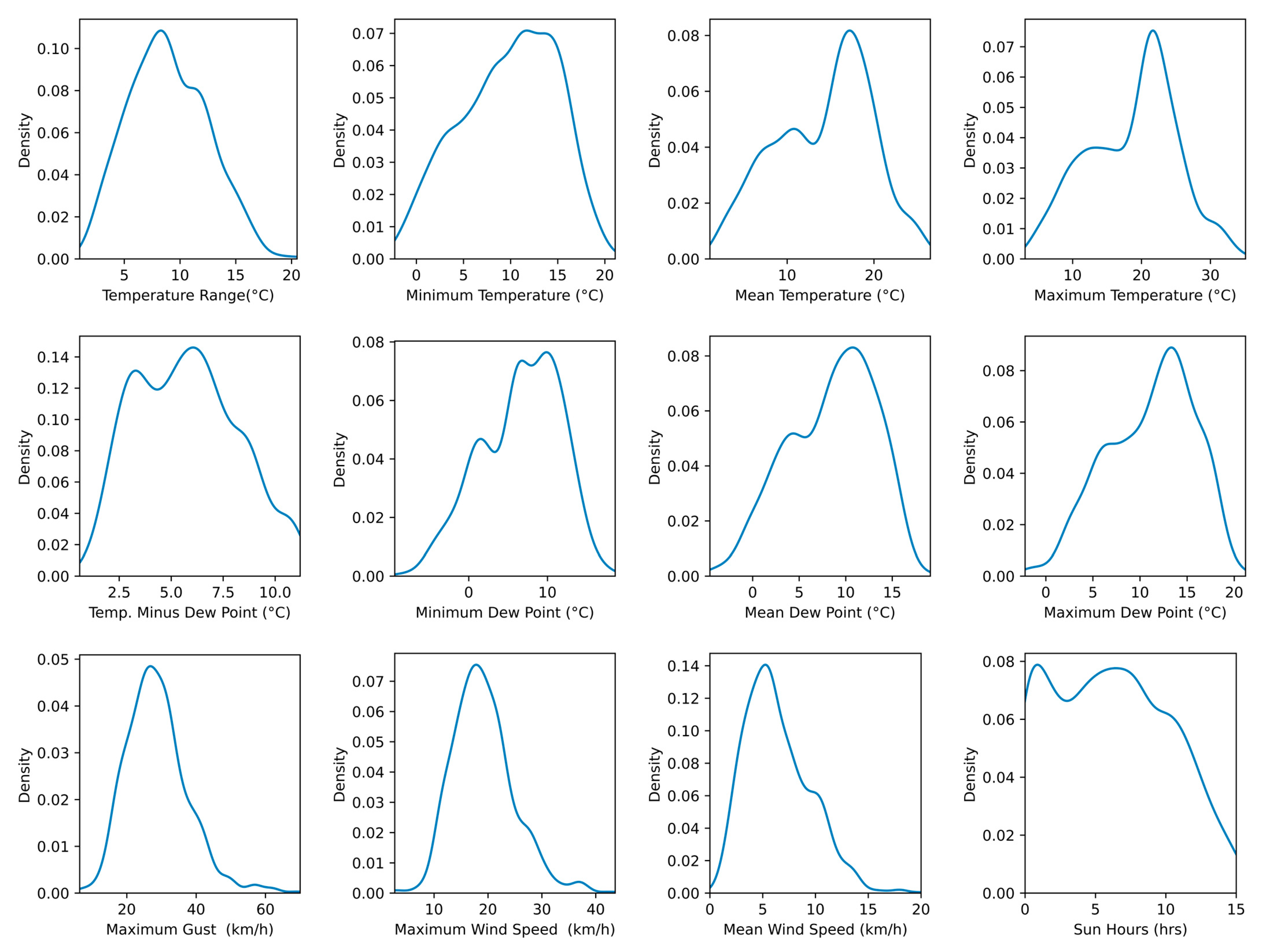
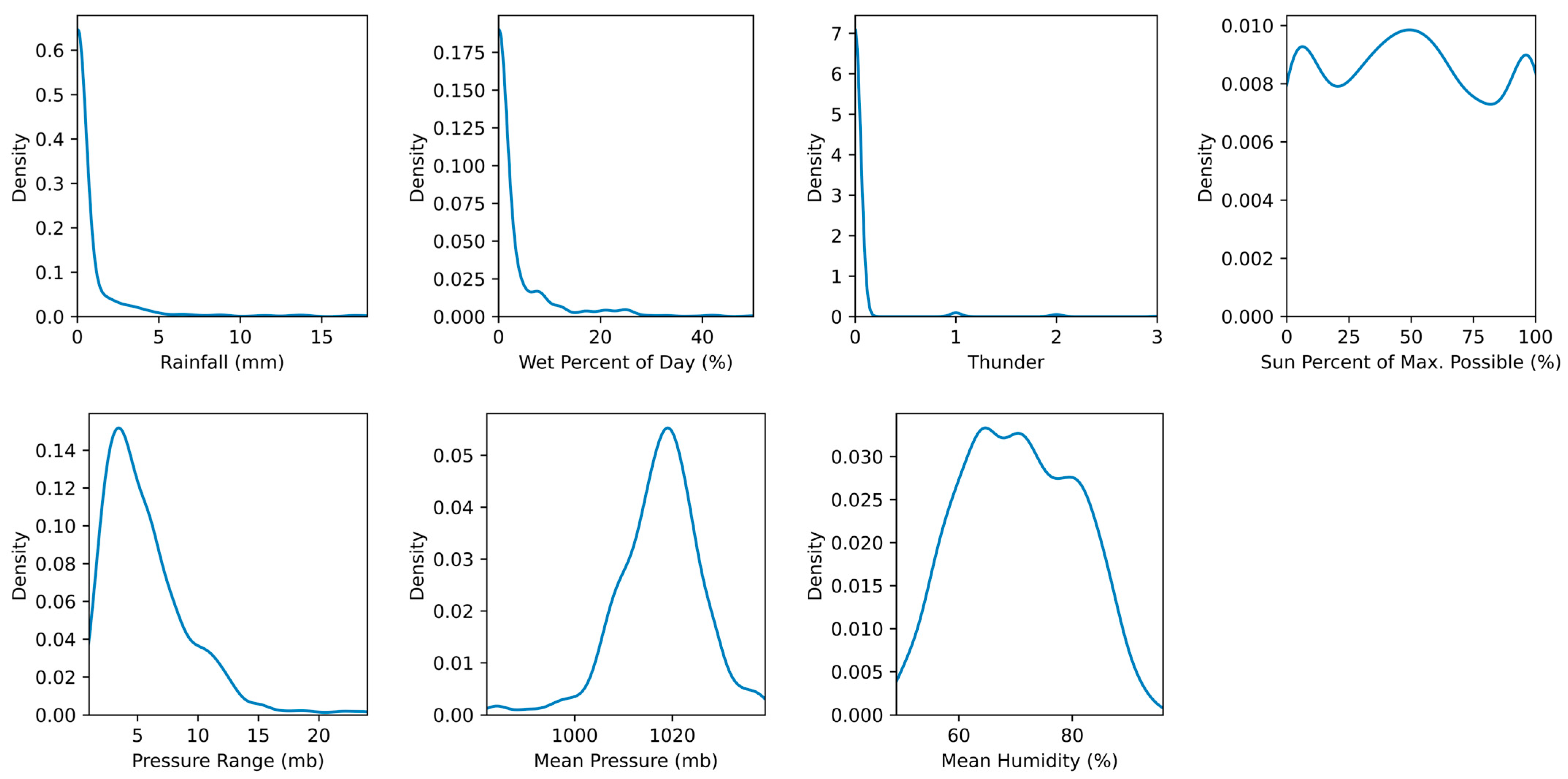
3.1.3. Weather Data Used for Both Datasets

As no historical weather data from the gliding sites were available, the data from a weather station in London have been used (http://nw3weather.co.uk, accessed on 13 October 2023). Eighteen different weather features were used: rainfall in mm per day, percent of the day with rainfall (wet percent of day), mean humidity, minimum/mean/maximum dew point, difference between the mean temperature and the mean dew point (temperature minus dew point), minimum/mean/maximum temperature, temperature range, mean pressure, pressure range, minimum/mean/maximum wind speed, maximum gust, strength of thunder, sun hours, and percent of sun hours from the possible sun hours. The strength of thunder was given as different categories (e.g., light, moderate, severe) and were converted into a scale for the purpose of this study.

3.2. Regression

Random forest (RF) regression was used to predict the flight duration. RFs are one of the most pertinent [32] ensemble machine learning technique [33,34]. As RFs are less prone to overfitting [33], this makes them an ideal choice for the task in hand. The features describing the flight (e.g., launch height and location) were constantly used. In addition, each combination of the 19 weather features, allowing for all possible sample sizes from one to nineteen (i.e., more than 500,000 combinations) were added to the model. The best combination, based on the mean absolute error (MAE), was used for the explainable AI.

TensorFlow [35], keras [36], sklearn [37] and keras_tuner [38] were used for the machine learning. The models were trained using a MacMini (Dual-Core Intel Core i5, 2.5 GHz, 16 GB RAM). The test dataset size was always 25% and the validation split was 20%. To ensure that the share of instances per class stayed the same across all datasets, the data were split in a stratified way. The libraries ‘seaborn’ [39] and ‘matplotlib’ [40] were used for the visualizations, alongside ‘numpy’ [41], and ‘pandas’ [42].

3.3. Classification

A random forest classifier was used to predict whether at least one flight on a given day managed to ‘get away’ (i.e., soared in a thermal for a sustained duration). Like the regression task, a RF was created for each combination of the 19 weather features. However, no flight-specific variables were used, as the focus was on whether the day was good enough to thermal and not on whether a specific flight ‘got away’. As four RFs shared the highest accuracy value, the RF which had the highest f1-value of those four was used.

3.4. Explainable Artificial Intelligence

Due to the ever-increasing complexity of machine learning models [43] and the move from symbolic AI systems to sub-symbolic systems [44], the research into explainable artificial intelligence (XAI) is growing rapidly [45]. An early version of this is a ‘decision tree’, which can provide individual explanations of the decision rules in, for example, classification tasks [46]. However, visualizing these for humans to easily understand would require limiting the scale of the decision tree to ensure interpretability at the sacrifice of precision. To avoid this [47], this paper uses SHAP (SHapley Additive exPlanations [48,49]), created by Lundberg and Lee. SHAP has been chosen as it is regarded as the ‘go-to’ feature importance XAI technique [50]. For the purpose of this study, SHAP is used to explain a model by illustrating the contribution of each individual feature to the prediction [50]. Following the suggestions by Thrun et al. [51], the goal was to explain the RF in a way that is understandable for experts in the subject (e.g., pilots), and not only by AI experts. XAI allows humans to ‘be in the loop’ [52], instead of blindly trusting machine learning models.

3.5. Limitations

A limitation of this study could be that the dataset is a real-world dataset and not specifically created for this study. However, this is also the main contribution of this study, as using real data from soaring flights is the best way to ensure that the models created work in reality.

4. Results

4.1. Regression (Prediction of Flight Duration)

4.1.1. Random Forest

The goal of the regression is to predict the flight duration. The best MAE, for the test dataset, is 5.74 min for the RF (

Table 1. The best RF with their MAE and features used.

				MAE in Minutes
Features *	5.74	5.76	5.76	5.76	5.77	5.79	5.79	5.80	5.80	5.81
Mean Wind Speed	X									X
Maximum Gust		X	X	X	X	X	X	X		X
Temperature Minus Dew Point	X	X	X	X	X	X	X	X	X	X
Maximum Dew Point		X						X
Mean Temperature							X
Maximum Temperature		X	X	X	X	X	X	X	X
Thunder	X	X	X		X		X			X
Rainfall			X
Wet percent of day	X	X	X	X	X	X	X	X	X	X
Mean Pressure			X		X	X			X
Pressure Range			X		X	X

* Weather features used in addition to the following features describing the flight: No time limit, Height, Rate of Sink, Airfield, Spin/Aerobatics, NrSeats, Failed.

). The best RF model includes only a few of the weather features. In the random forest, the feature that is always used in the top 10 results is the ‘wet percent’ of the day and the difference between the temperature and the dew point.

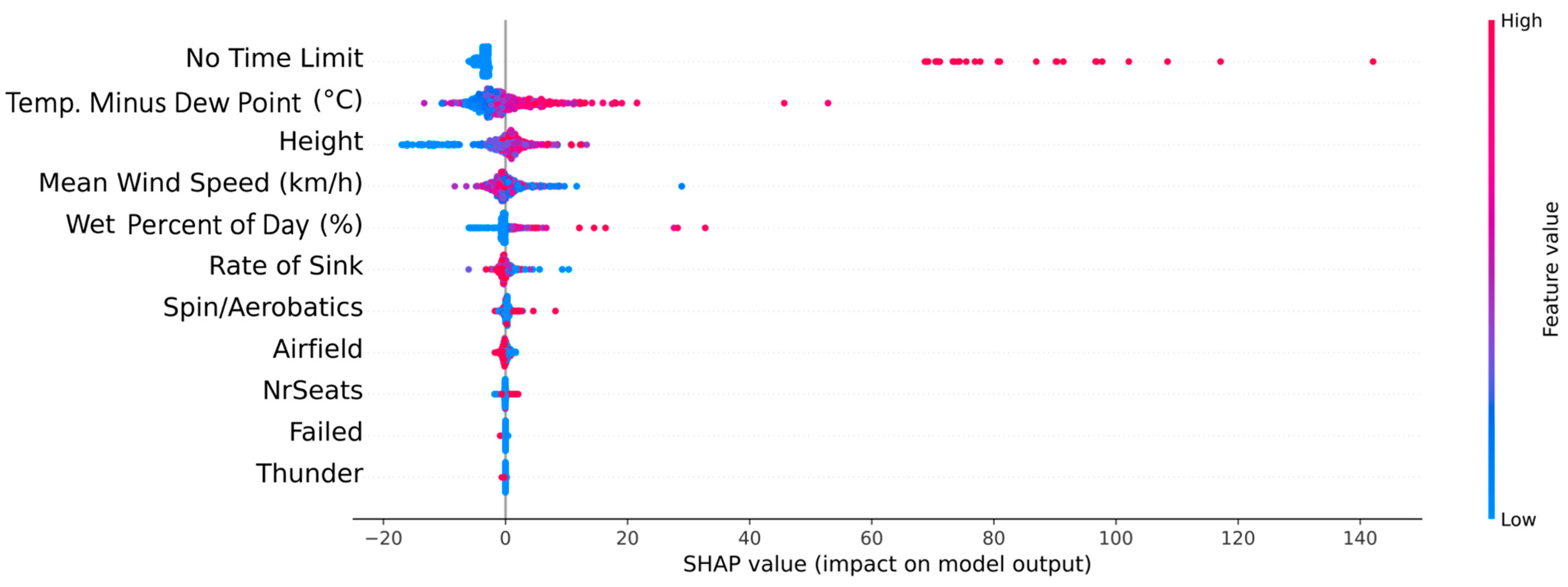
4.1.2. Explainable Artificial Intelligence (SHapley Additive exPlanations; SHAP)

The feature importance for the best RF regressors is shown in Figure 1. Obviously, whether the flight duration was permitted to be longer than 60 min (‘No time limit’) is the most important feature. This was included as, at most gliding clubs, the flight duration is usually limited to around 1 h, to ensure that all members have a fair opportunity to fly. For badge claim flights (i.e., 50 km, 5 h) or when there is no demand for the glider, longer flights are possible. The difference between the temperature and the dew point is the second most important feature, which will not be a surprise in gliding circles, as this is a commonly used value to identify the best time to fly. The launch height has a significant influence on the flight duration as well.

SHAP has been used in this study to gain an understanding of each feature’s contribution to the RF model [50]. Figure 2 shows the global feature contribution on the prediction of the RF. The y-axis illustrates the hierarchical order of the features in the RF. For each feature, a horizontal distribution of the SHAP values are displayed. A negative impact is shown as <0 and a positive impact is shown as >0. The blue colour represents a low feature value, purple is an average value, and the red is high.

The flight duration is clearly extended dramatically if there is no time limit, while having one reduces the flight time slightly.

If the difference between the temperature and dew point is significant, then the flight time is increased: a fact that will not surprise glider pilots. For the interested non-pilot, the dew point is the temperature when a given airmass becomes saturated. Together with the temperature, the dew point can be used to calculate the height of the cloud base (see Equation (2) [53]. The higher a glider pilot can ascend, the more chances there are to reach the next thermal and increase their flight time.

$$h_{cloud}=\frac{\left(t-d\right)}{2.5}\times 1000$$

(2)

where:

$h_{cloud}$ is the height of the cloud base layer (ft);

$t$ is the temperature (°C);

$d$ is the dew point (°C).

A higher release height in the launch generally increases the flight duration, as the tow (i.e., when the glider is on tow) takes longer. After release, a higher launch height facilitates multiple opportunities to encounter thermals and staying airborne in the absence of any thermal activity. However, some of these extra high launches (3000 ft to 4000 ft) are also used for aerobatic training which, apart from the 15–20 min launch window, are rather shorter in duration. Flights with the intended purpose of soaring in thermals are commonly launched to 2000 ft. This explains why both the red and purple points (high launches/standard launches) can be found extending the flight duration, while other red and purple markers influence the duration slightly. The purpose of low launch heights, around 1000 ft to 1500 ft, is to practice take-off, circuit, approach, and landing and, therefore, the result of these is a relatively short flight.

It is more difficult to centre in a thermal when the wind is stronger and, therefore, the probability is that there will be a reduction in the overall flight time. Also, pilots may need to leave the thermal earlier to stay within range of the airfield, as the wind pushes the glider downwind.

Flying is cancelled on a rainy day. Therefore, the average ‘wet percent of the day’ is only 2.65% in the dataset. So, even a day where it rained 4% of the time is considered a high value by this model. As glider pilots in the UK know, a brief shower is not always the end of the flying day. In fact, it may ultimately be a good day before and after a frontal system moves through. The risk of rain keeps the demand for gliders low, while there still may be good thermal activity in the local area at other times of the day. It is not surprising that the flight time is expected to increase when the ‘wet percent of the day’ is higher than 2.65%. Such a low ‘wet percent of the day’ still leaves plenty of hours for flying without precipitation.

The higher the rate of sink of the glider, the shorter the flight; and that is certainly no surprise.

Participating in aerobatics during a flight reduces or increases the flight time, as there are two different types of aerobatic flights: (i) formal aerobatic training flights, launched to 3000 ft to 4000 ft, which are usually only 20 min long, and (ii) unexpected soaring flights, where the instructor uses aerobatic manoeuvres, such as a loop, to lose altitude, in order to shorten the flight so that a student waiting on the ground can also fly.

The two different airfields where the flights were launched do not adversely influence the results. However, it can be observed that the flights are slightly longer at one location; this is perhaps due to the terrain of the surrounding countryside.

Figure 3 illustrates density plots of the weather features used in this study. Flights took place across the whole year, even on cold winter’s days. While on most flying days, no rain was reported, a brief shower certainly does not end the flying activity. The average wind speed was generally less than 20 km/h (11 knots). Flights took place during full and partial cloud cover, as well as on blue sunny days.

4.2. Classification Task

4.2.1. Classification Task

A RF classifier has been trained to predict, based on the weather, the likelihood that at least one flight soared in thermals successfully on a given day. The highest accuracy of the test dataset is 81.2% (

Table 2. The best RF with their accuracy and features used.

	Accuracy
Features	0.812 *	0.812	0.812	0.812	0.797	0.797	0.797	0.797	0.797	0.797
Mean Wind Speed										X
Maximum Wind Speed	X	X	X	X	X	X	X	X	X	X
Temperature Minus Dew Point							X			X
Minimum Dew Point									X
Mean Dew Point			X		X	X		X		X
Maximum Dew Point	X			X
Maximum Temperature	X
Minimum Temperature		X	X						X
Mean Humidity	X	X	X	X	X	X	X	X	X	X
Sun Percent of Max Possible	X	X	X		X	X	X	X	X
Sun Hours	X	X		X	X	X		X	X
Thunder	X		X					X	X
Wet Percent of Day	X	X			X		X	X		X
Rainfall	X	X		X		X	X	X	X	X
Mean Pressure		X	X			X		X	X	X
Pressure Range	X			X	X		X		X	X

* used for the explainable AI.

). Interestingly, the difference between the temperature and the dew point (i.e., indicating the hight of the thermals) is not a commonly used weather feature. While the flight duration largely depends on the thermal height, whether it is possible to thermal on a given day depends on other features. Humidity and maximum wind speed are most commonly used. It may appear as if each RF uses a completely different set of features; however, in most cases, only the minimal value (e.g., minim temperature) is replaced by the mean or maximum value (e.g., maximum temperature), or vice versa.

4.2.2. Explainable Artificial Intelligence (SHapley Additive exPlanations; SHAP)

The mean humidity is the most important feature (Figure 4); therefore, it is not surprising that it is used in all top 10 RF classifiers (Table 2). Maximum temperature is the second most important feature, followed by the maximum wind speed.

As can be seen in Figure 5, the lower the humidity, the higher the chances for the glider to ‘get away’ (i.e., soaring in thermals successfully). If the air is saturated with cold moisture it takes longer to warm, and, therefore, there are fewer opportunities to trigger a rising airmass.

A higher temperature increases the likelihood that there will be at least one flight in a thermal during the day. This is expected, given that it is far more likely to have a good day of soaring in thermals in spring and autumn, while it is rather unusual to encounter thermals in winter. However, hot temperatures are not a guarantee of a good thermal day. Only low temperatures (i.e., blue dots) reduce the chance of ‘getting away’, while medium and high temperatures (i.e., purple and red) may or may not increase the likelihood of a good soaring day (i.e., located around 0 and +0.1 in Figure 5).

As said before, lower windspeeds make it easier to centre in thermals and therefore increase the likelihood of a good thermal flight.

A low dew point reduces the likelihood of a flight in thermals, as does a low temperature.

If there are only a few hours of sunshine per day, as seen in winter or under a thick layer of cloud in summer, thermals are generally inhibited and may switch off before recycling. For the percent of maximum sun possible, some of the extreme values are seen on the left-hand side of the figure, as both clear winter days and overcast days make soaring in thermals improbable. The best time to soar in thermals is in the spring and autumn, when clouds are indicating possible locations of soaring opportunities. While it is possible to bump into a thermal on a summer’s day without any clouds, more experience or luck may be required.

There is no very clear indication of the effect of the pressure differential during the day. Completely static pressure may reduce the chance of thermals developing; however, there is no obvious trend.

As explained before, ‘high’ rainfall and a ‘high’ wet percent increases the likelihood of a flight in thermals, simply because a ‘high’ wet percent only refers to above 2.4%, as no flying will take place when it is raining for most parts of the day. If there is a high chance of thunder, flying is stopped for safety concerns, and, therefore, it reduces the likelihood of ‘getting away’.

5. Discussion

The explanations of the models derived from SHAP are in line with common glider pilot knowledge. The study also highlights the importance of combining XAI with human knowledge to gain a holistic understanding of the model, to avoid misinterpretation.

A higher release height in the launch can be used to predict the flight duration; however, as evidenced by the SHAP values, it is not a linear relationship. Some of these extra high launches (3000 ft to 4000 ft) are used for aerobatic training flights. The duration of these is close to the average flight time. The actual free flight time being curtailed with aerobatics is compensated for, by the longer period spent on tow (15–20 min). Some of the extra high launches are also used for thermal training and, therefore, have greater durations. Flights with the intended purpose of soaring in thermals or general tuition are commonly launched to 2000 ft. Some might ‘get away’ and have a longer flight, while others do not. The purpose of low launch heights, around 1000 ft to 1500 ft, is to practice take-off and landing and, therefore, almost always result in short flights.

It is certainly no surprise that a higher rate of sink of the glider reduces the flight duration.

According to the SHAP summary plot, aerobatics both increases and reduces the flight time. The correct interpretation of this fact requires knowledge of the way the ‘pilot in command’ teaches students. There are two different types of instructional aerobatic flights: (i) flights as part of an aerobatic training course, launched between 3000 ft and 4000 ft, and (ii) unexpected soaring flights, where the instructor uses aerobatic manoeuvres to lose altitude and end the flight, giving others the chance to fly. The latter is clearly indicative of a longer flight duration, while the first examples are usually only 20–25 min long. This is clearly visible in the SHAP summary plot but requires additional knowledge beyond the dataset to understand this factor.

The difference between the temperature and dew point provides a clear indication of the flight duration. It is indicative of the cloud height and, therefore, the height of thermals. Higher thermals increases the possible height gain resulting into more opportunities to reach other active thermals. However, the height of thermals has no bearing on whether at least one glider manged to find a thermal on a given day.

Wind is an important factor for both the flight duration and whether soaring in thermals was possible. It is more difficult to centre in the thermal when the wind is strong, and pilots may need to leave the thermal earlier to stay within range of the airfield, as the glider is pushed downwind.

The fact that, according to SHAP, higher amounts of rain increase soaring capabilities may be surprising, as most would expect the opposite. However, flying is cancelled on a rainy day. There are no flying data from rainy days in this dataset. Therefore, the average ‘wet percent of the day’ in this dataset is only 2.65%. Even just 4% of rain is considered a high value. As glider pilots in the UK know, a brief shower is not the end of the flying day. In fact, it may ultimately be a good day before and after a frontal system moves through. Also, the possibility of rain keeps the demand for gliders low and therefore offers more opportunities to soar in thermals. This example highlights that it is important to know the dataset and its peculiarities before trying to understand the results of an explainable AI.

The humidity, temperature and sunshine are not necessarily key features used by the RF regression, but they are important for the classification task.

A lower humidity increases the likelihood that at least one glider managed to find a thermal on a given day.

Obviously, most soaring in thermals takes place in the warmer season. A higher temperature increases the likelihood that there will be at least one flight in thermals on the day. However, a high temperature is no guarantee of an increase in thermal-soaring capabilities, but a low temperature makes finding a thermal improbable, which can clearly be seen on the SHAP summary plot.

In general, thermals are unable to fully develop with only a few hours of sun per day in the winter or under a thick cloud layer in summer. The best time to find a thermal is generally during the warmer months of the year, when the sun has enough strength to heat the ground. Clouds are an indication of the possible track and final location of thermals, which makes finding thermals more predictable. While it is possible to simply bump into a thermal on a blue summer’s day, more skill or luck is required. All these factors can be seen in the SHAP plot.

6. Conclusions

The paper has two main contributions: first, the paper illustrates why explainable AI needs to be combined with human knowledge of both the subject as well as the peculiarities in the dataset, to avoid misinterpretations. Secondly, the paper contributes to the published research by predicting the soaring capabilities of sailplanes using data from real instructional glider flights. The latter goal (i.e., gliding site optimisation and understanding the influence of weather on the operational management of a soaring UAV fleet) has not yet attracted significant attention in the public domain. Published papers have mainly focused on investigating the use of soaring in thermals to extend the flight of UAVs as well as methods (i.e., control algorithms) to enable an aircraft to soar like a bird.

The RF regressor, which predicts the flight duration, achieved an MAE of 5.7 min. The RF classifier, which predicts the probability that at least one flight was a flight in thermals on a given day, has an accuracy of 81.2%.

The explanations of the models derived from SHAP (SHapley Additive exPlanations) are in line with the common knowledge of experienced glider pilots. The influence of features like the wind strength, humidity and the difference between temperature and dew point are all within the shared vocabulary of an experienced glider pilot. However, the study also highlights the dangers of relying solely on the explanation offered by an explainable AI. Instead, it is important to combine explainable AI with human knowledge to gain a holistic understanding. Both the range of situations covered by the dataset as well as subject expertise (e.g., glider pilots) need to be appreciated to avoid misinterpretations. For example, correctly interpreting the assertion by SHAP that more rain increases the ability to soar requires the knowledge that no flying takes place when it rains all day and that these days are, therefore, not included in the dataset. A frontal system moving through the area may come with slight rain but could bring favourable thermal-soaring opportunities. Interpreting the effect of aerobatic manoeuvres on flight durations (i.e., both increasing and reducing the flight time) requires knowledge of the instructor’s way of teaching, to understand the explanations given by SHAP.

This study uses actual weather observations for their prediction. As the next step, the machine learning models should be trained on weather forecasts instead of real observations. Doing so would ensure that the models are able to predict the potential soaring capabilities of the following day.

References

1. Lawrance, N.R.J.; Sukkarieh, S. A guidance and control strategy for dynamic soaring with a gliding UAV. In Proceedings of the 2009 IEEE International Conference on Robotics and Automation, Kobe, Japan, 12–17 May 2009; IEEE: Piscataway, NJ, USA, 2009. [Google Scholar]
2. Gao, X.-Z.; Hou, Z.-X.; Guo, Z.; Fan, R.-F.; Chen, X.-Q. Analysis and design of guidance-strategy for dynamic soaring with UAVs. Control Eng. Pract. 2014, 32, 218–226. [Google Scholar] [CrossRef]
3. White, C.; Lim, E.; Watkins, S.; Mohamed, A.; Thompson, M. A feasibility study of micro air vehicles soaring tall buildings. J. Wind Eng. Ind. Aerodyn. 2012, 103, 41–49. [Google Scholar] [CrossRef]
4. Kim, S.-H.; Lee, J.; Jung, S.; Lee, H.; Kim, Y. Deep neural network-based feedback control for dynamic soaring of unpowered aircraft. IFAC-PapersOnLine 2019, 52, 117–121. [Google Scholar] [CrossRef]
5. Chudej, K.; Klingler, A.-L.; Britzelmeier, A. Flight path optimization of a hang-glider in a thermal updraft. IFAC-PapersOnLine 2015, 48, 808–812. [Google Scholar] [CrossRef]
6. Schermann, E.; Omran, H.; Durand, S.; Kiefer, R. Stochastic trajectory optimization for autonomous soaring of UAV. IFAC-PapersOnLine 2019, 52, 562–567. [Google Scholar] [CrossRef]
7. Rejeb, A.; Abdollahi, A.; Rejeb, K.; Treiblmaier, H. Drones in agriculture: A review and bibliometric analysis. Comput. Electron. Agric. 2022, 198, 107017. [Google Scholar] [CrossRef]
8. Edulakanti, S.R.; Ganguly, S. Review article: The emerging drone technology and the advancement of the Indian drone business industry. J. High Technol. Manag. Res. 2023, 34, 100464. [Google Scholar] [CrossRef]
9. de Villiers, C.; Munghemezulu, C.; Mashaba-Munghemezulu, Z.; Chirima, G.J.; Tesfamichael, S.G. Weed Detection in Rainfed Maize Crops Using UAV and PlanetScope Imagery. Sustainability 2023, 15, 13416. [Google Scholar] [CrossRef]
10. Mndela, Y.; Ndou, N.; Nyamugama, A. Irrigation Scheduling for Small-Scale Crops Based on Crop Water Content Patterns Derived from UAV Multispectral Imagery. Sustainability 2023, 15, 12034. [Google Scholar] [CrossRef]
11. Hafeez, A.; Husain, M.A.; Singh, S.; Chauhan, A.; Khan, M.T.; Kumar, N.; Chauhan, A.; Soni, S. Implementation of drone technology for farm monitoring & pesticide spraying: A review. Inf. Process. Agric. 2023, 10, 192–203. [Google Scholar] [CrossRef]
12. Hart, L.; Quendler, E.; Umstaetter, C. Sociotechnological Sustainability in Pasture Management: Labor Input and Optimization Potential of Smart Tools to Measure Herbage Mass and Quality. Sustainability 2022, 14, 7490. [Google Scholar] [CrossRef]
13. Coutinho, W.P.; Fliege, J.; Battarra, M. Glider Routing and Trajectory Optimisation in disaster assessment. Eur. J. Oper. Res. 2019, 274, 1138–1154. [Google Scholar] [CrossRef]
14. Maqbool, A.; Mirza, A.; Afzal, F.; Shah, T.; Khan, W.Z.; Bin Zikria, Y.; Kim, S.W. System-Level Performance Analysis of Cooperative Multiple Unmanned Aerial Vehicles for Wildfire Surveillance Using Agent-Based Modeling. Sustainability 2022, 14, 5927. [Google Scholar] [CrossRef]
15. Josipovic, N.; Viergutz, K. Smart Solutions for Municipal Flood Management: Overview of Literature, Trends, and Applications in German Cities. Smart Cities 2023, 6, 944–964. [Google Scholar] [CrossRef]
16. Munawar, H.S.; Ullah, F.; Qayyum, S.; Heravi, A. Application of deep learning on uav-based aerial images for flood detection. Smart Cities 2021, 4, 1220–1242. [Google Scholar] [CrossRef]
17. Runnström, M.C.; Ólafsdóttir, R.; Blanke, J.; Berlin, B. Image analysis to monitor experimental trampling and vegetation recovery in icelandic plant communities. Environments 2019, 6, 99. [Google Scholar] [CrossRef]
18. Cagnazzo, C.; Potente, E.; Regnauld, H.; Rosato, S.; Mastronuzzi, G. Autumnal beach litter identification by mean of using ground-based ir thermography. Environments 2021, 8, 37. [Google Scholar] [CrossRef]
19. Rachmawati, T.S.N.; Kim, S. Unmanned Aerial Vehicles (UAV) Integration with Digital Technologies toward Construction 4.0: A Systematic Literature Review. Sustainability 2022, 14, 5708. [Google Scholar] [CrossRef]
20. Chen, Y.-C.; Huang, C. Smart data-driven policy on unmanned aircraft systems (UAS): Analysis of drone users in U.S. cities. Smart Cities 2021, 4, 78–92. [Google Scholar] [CrossRef]
21. Kharchenko, V.; Kliushnikov, I.; Rucinski, A.; Fesenko, H.; Illiashenko, O. UAV Fleet as a Dependable Service for Smart Cities: Model-Based Assessment and Application. Smart Cities 2022, 5, 1151–1178. [Google Scholar] [CrossRef]
22. Karakikes, I.; Nathanail, E. Using the delphi method to evaluate the appropriateness of urban freight transport solutions. Smart Cities 2020, 3, 1428–1447. [Google Scholar] [CrossRef]
23. Wang, Y.; Kumar, L.; Raja, V.; Al-Bonsrulah, H.A.Z.; Kulandaiyappan, N.K.; Tharmendra, A.A.; Marimuthu, N.; Al-Bahrani, M. Design and Innovative Integrated Engineering Approaches Based Investigation of Hybrid Renewable Energized Drone for Long Endurance Applications. Sustainability 2022, 14, 16173. [Google Scholar] [CrossRef]
24. Lee, D.; Longo, S.; Kerrigan, E.C. Predictive control for soaring of unpowered autonomous UAVs. IFAC Proc. Vol. 2012, 45, 194–199. [Google Scholar] [CrossRef]
25. Camacho, N.; Dobrokhodov, V.N.; Jones, K.D. Cooperative Autonomy of Multiple Solar-Powered Thermaling Gliders⋆. In Proceedings of the 19th World Congress the International Federation of Automatic Control, Cape Town, South Africa, 24–29 August 2014. [Google Scholar]
26. Teodoro, A.; Santos, P.; Marques, J.E.; Ribeiro, J.; Mansilha, C.; Melo, A.; Duarte, L.; de Almeida, C.R.; Flores, D. An integrated multi-approach to environmental monitoring of a self-burning coal waste pile: The são pedro da cova mine (porto, portugal) study case. Environments 2021, 8, 48. [Google Scholar] [CrossRef]
27. Dickmanns, E. Collocated Hermite Approximation Applied to Time Optimal Crosscountry Soaring. IFAC Proc. Vol. 1983, 16, 137–145. [Google Scholar] [CrossRef]
28. Cui, Y.; Yan, D.; Wan, Z. Study on the Glider Soaring Strategy in Random Location Thermal Updraft via Reinforcement Learning. Aerospace 2023, 10, 834. [Google Scholar] [CrossRef]
29. Harzer, J.; De Schutter, J.; Diehl, M.; Meyers, J. Dynamic soaring in wind turbine wakes. Eur. J. Control. 2023, 74, 100842. [Google Scholar] [CrossRef]
30. Thakker, D.; Mishra, B.K.; Abdullatif, A.; Mazumdar, S.; Simpson, S. Explainable artificial intelligence for developing smart cities solutions. Smart Cities 2020, 3, 1353–1382. [Google Scholar] [CrossRef]
31. Englund, C.; Aksoy, E.; Alonso-Fernandez, F.; Cooney, M.; Pashami, S.; Åstrand, B. AI perspectives in smart cities and communities to enable road vehicle automation and smart traffic control. Smart Cities 2021, 4, 783–802. [Google Scholar] [CrossRef]
32. You, J.; van der Klein, S.A.; Lou, E.; Zuidhof, M.J. Application of random forest classification to predict daily oviposition events in broiler breeders fed by precision feeding system. Comput. Electron. Agric. 2020, 175, 105526. [Google Scholar] [CrossRef]
33. Breiman, L. Random forests. Mach. Learn. 2001, 45, 5–32. [Google Scholar] [CrossRef]
34. Genuer, R.; Poggi, J.; Tuleau-Malot, C. Variable selection using random forests. Pattern Recognit. Lett. 2010, 31, 2225–2236. [Google Scholar] [CrossRef]
35. Abadi, M.; Agarwal, A.; Barham, P.; Brevdo, E.; Chen, Z.; Citro, C.; Corrado, G.S.; Davis, A.; Dean, J.; Devin, M.; et al. TensorFlow: Large-Scale Machine Learning on Heterogeneous Distributed Systems. Available online: www.tensorflow.org (accessed on 2 July 2023).
36. Gulli, A.; Pal, S. Deep Learning with Keras. Available online: https://keras.io (accessed on 2 July 2023).
37. Pedregosa, F.; Varoquaux, G.; Gramfort, A.; Michel, V.; Thirion, B.; Grisel, O.; Blondel, M.; Prettenhofer, P.; Weiss, R.; Dubourg, V.; et al. Scikit-Learn: Machine Learning in Python. 2011. Available online: http://scikit-learn.sourceforge.net (accessed on 2 July 2023).
38. O’Malley, T.; Bursztein, E.; Long, L.; Chollet, F.; Jin, H.; Invernizzi, L. KerasTuner. Available online: https://github.com/keras-team/keras-tuner (accessed on 2 July 2023).
39. Waskom, M.; Botvinnik, O.; Hobson, P.; Cole, J.B.; Halchenko, Y.; Hoyer, S.; Miles, A.; Augspurger, T.; Yarkoni, T.; Megies, T.; et al. Seaborn: v0.5.0 (November 2014). Available online: https://zenodo.org/records/12710 (accessed on 2 July 2023).
40. Hunter, J.D. Matplotlib: A 2D Graphics Environment. Comput. Sci. Eng. 2007, 9, 90–95. [Google Scholar] [CrossRef]
41. Harris, C.R.; Millman, K.J.; van der Walt, S.J.; Gommers, R.; Virtanen, P.; Cournapeau, D.; Wieser, E.; Taylor, J.; Berg, S.; Smith, N.J.; et al. Array programming with NumPy. Nature 2020, 585, 357–362. [Google Scholar] [CrossRef] [PubMed]
42. McKinney, W. Data Structures for Statistical Computing in Python. In Proceedings of the 9th Python in Science Conference, Austin, TX, USA, 28 June–3 July 2010. [Google Scholar]
43. Rosenberg, G.; Brubaker, J.K.; Schuetz, M.J.A.; Salton, G.; Zhu, Z.; Zhu, E.Y.; Kadıoğlu, S.; Borujeni, S.E.; Katzgraber, H.G. Explainable Artificial Intelligence Using Expressive Boolean Formulas. Mach. Learn. Knowl. Extr. 2023, 5, 1760–1795. [Google Scholar] [CrossRef]
44. Cabitza, F.; Campagner, A.; Natali, C.; Parimbelli, E.; Ronzio, L.; Cameli, M. Painting the Black Box White: Experimental Findings from Applying XAI to an ECG Reading Setting. Mach. Learn. Knowl. Extr. 2023, 5, 269–286. [Google Scholar] [CrossRef]
45. Kim, M.-Y.; Atakishiyev, S.; Babiker, H.K.B.; Farruque, N.; Goebel, R.; Zaïane, O.R.; Motallebi, M.-H.; Rabelo, J.; Syed, T.; Yao, H.; et al. A Multi-Component Framework for the Analysis and Design of Explainable Artificial Intelligence. Mach. Learn. Knowl. Extr. 2021, 3, 900–921. [Google Scholar] [CrossRef]
46. Buhrmester, V.; Münch, D.; Arens, M. Analysis of Explainers of Black Box Deep Neural Networks for Computer Vision: A Survey. Mach. Learn. Knowl. Extr. 2021, 3, 966–989. [Google Scholar] [CrossRef]
47. Trebbien, J.; Gorjão, L.R.; Praktiknjo, A.; Schäfer, B.; Witthaut, D. Understanding electricity prices beyond the merit order principle using explainable AI. Energy AI 2023, 13, 100250. [Google Scholar] [CrossRef]
48. Lundberg, S.M.; Erion, G.; Chen, H.; DeGrave, A.; Prutkin, J.M.; Nair, B.; Katz, R.; Himmelfarb, J.; Bansal, N.; Lee, S.-I. From local explanations to global understanding with explainable AI for trees. Nat. Mach. Intell. 2020, 2, 56–67. [Google Scholar] [CrossRef]
49. Lundberg, S.M.; Allen, P.G.; Lee, S.-I. A Unified Approach to Interpreting Model Predictions. Available online: https://github.com/slundberg/shap (accessed on 2 July 2023).
50. Utama, C.; Meske, C.; Schneider, J.; Schlatmann, R.; Ulbrich, C. Explainable artificial intelligence for photovoltaic fault detection: A comparison of instruments. Sol. Energy 2023, 249, 139–151. [Google Scholar] [CrossRef]
51. Thrun, M.C.; Ultsch, A.; Breuer, L. Explainable AI Framework for Multivariate Hydrochemical Time Series. Mach. Learn. Knowl. Extr. 2021, 3, 170–204. [Google Scholar] [CrossRef]
52. Lohaj, O.; Paralič, J.; Bednár, P.; Paraličová, Z.; Huba, M. Unraveling COVID-19 Dynamics via Machine Learning and XAI: Investigating Variant Influence and Prognostic Classification. Mach. Learn. Knowl. Extr. 2023, 5, 1266–1281. [Google Scholar] [CrossRef]
53. Hawkins, C. How to Estimate Cloud Bases and Heights. Available online: https://www.flymac.co.uk/how-to-estimate-cloud-bases-and-heights/ (accessed on 11 October 2023).
Figure 1. Feature importance.
Smartcities 07 00007 g001
Figure 2. SHAP summary plot (regression: flight duration).
Smartcities 07 00007 g002
Figure 3. Weather range for the flying days.
Smartcities 07 00007 g003aSmartcities 07 00007 g003b
Figure 4. SHAP feature importance (classification).
Smartcities 07 00007 g004
Figure 5. SHAP summary plot (classification: was there at least one flight soaring in a thermal on a given day?).
Smartcities 07 00007 g005