Turbulence Models Studying the Airflow around a Greenhouse Based in a Wind Tunnel and Under Different Conditions

Abstract

Turbulence phenomena created around a greenhouse due to different wind loads are key factors in its structural design and significantly affect the ventilation rates through its side and roof openings. Using the turbulence models of ANSYS FLUENT software to investigate the airflow around an arched-roof-greenhouse-shaped obstacle placed inside a wind tunnel was the aim of this study. Velocity and pressure areas around the obstacle were examined by selecting three different turbulence models (Standard, RNG and Realizable k–ε models) under three different airflow entry velocities (0.34, 1.00 and 10.00 m s⁻¹) in the wind tunnel. All k–ε models showed that when the air velocity was intensified, the airflow was identified as turbulent. The horizontal velocity profile predicted more accurately the presence of vortices in contrast with the vector sum of the perpendicular velocity components. Vortices were formed upstream, above the roof and downstream of the obstacle, and the applied models showed that when airflow velocity increases, the size of the upstream vortex decreases. Finally, there was a strong indication from the modeling results that the vortex on the roof of the obstacle was an extension of the vortex that was created downstream.

1. Introduction

Studying the airflow around and over an agricultural structure (greenhouse, livestock unit, etc.) could possibly resolve substantial issues related to the proper functioning of these structures. Ventilation is an important factor strongly interconnected with the regulation of the microenvironment and performance of an agricultural structure. In greenhouses, ventilation affects temperature, humidity and CO₂ concentration, and in livestock buildings it is important for minimizing the concentrations of harmful gases (NH₃, CO₂, CH₄, N₂O, etc.) that have adverse effects on the wellbeing of animal and workers [1,2,3,4].

Until recently, most research efforts concentrated on studying the airflow through modeling using computational fluid mechanics for openings in specific locations, mainly on the side surfaces of greenhouses. However, these openings can cause damage to the materials of the building if the wind is stronger than the air speed limit set by the manufacturer. As is well known, the equations that govern the dynamic behavior of fluids are the Navier–Stokes (N–S) equations, which are the basis of modeling through computational fluid dynamics [4,5,6]. In contrast to the direct numerical simulation, which solves the N–S equations without simplifications, the models provided by ANSYS FLUENT [1,7,8,9,10,11], are “obliged” to make some simplifications for solving these equations. Therefore, the respective results are decisively influenced by the choice of each model.

The available literature on computational fluid dynamics focuses mainly on points that need special attention when the analysis is performed using commercial packages, such as ANSYS FLUENT. Specifically, the quality of the grid and the management of the boundary conditions are of paramount importance for a reliable analysis. In terms of grid quality, Roache [12] introduced a grid convergence index (GCI). The proposed method provides an asymptotic approach to quantifying the uncertainty in lattice convergence. Important observations on the most reliable analysis of flow fields using commercial packages are given in the review conducted by Murakami [13,14]. Guidelines are given when dealing with marginal conditions at obstacles, and generally at impermeable surfaces. It is pointed out that the logarithmic area function (wall function) does not give satisfactory results when the flow area is to be investigated in the presence of a detachment. In this case the partial function Χn + is suggested with different functions for the linear area region (non-slip) and for the free flow area. is the authors found that the two main problems when dealing with turbulence modeling are the high Re numbers that cause the grid to thicken, and the phenomenon of clashing flow lines at the front of the obstacle. The validity of modeling a three-dimensional airflow in an air tunnel using RANS packages for all the common roof designs of greenhouses was investigated by Ntinas et al. [8]. An air tunnel experiment was also conducted for better validation of the used models, and the results showed that in all cases the maximum speeds appeared at the top of the construction. Although the results in terms of velocity profiles and turbulent kinetic energy results are similar, in the study, the RNG k–ε model predicted the air speed best, and the SST k–ω model was the most suitable for calculating the turbulent kinetic energy accurately. As was expected, the modeling failed to simulate the area downstream of the obstacle as the flow field was chaotic.

Apart from the studies done for the airflow around and over a greenhouse, a lot of research has been conducted for modelling the airflow inside a greenhouse. The aim of these studies was to achieve efficient ventilation by the creation of appropriate air currents that were not harmful for plants and were effective at cooling greenhouses. The effect of wind speed on the natural ventilation of a greenhouse using ANSYS/FLOATRAN was studied by Molina et al. [15]. This study included airflow and temperature distribution, and the results highlighted the importance of roof openings for proper ventilation. Side openings of the greenhouse increased the thermal lift. Moreover, Ould Khaoua et al. [16] investigated the roof openings configuration of a naturally ventilated greenhouse, and reported that openings in the windward part of the roof create more efficient ventilation. Kuroyanagi [10] studied the pressure profile developed around a greenhouse due to wind with the help of CFD and estimated the escape airflow for different orientations and air speeds. The calculation of the pressure coefficient inside the greenhouse was obtained from the value of the corresponding coefficient in the outdoor area, which was found by the CFD analysis.

The distances between multiple greenhouse units have significant effects on the airflow distribution, and many researchers have studied the development of turbulent flow through the vortices that occur within greenhouses.

From the above literature it can be concluded that the correct and accurate modeling of turbulence through commercial computer packages is a process which requires the correct choice of model and the researcher’s experience about the limits of the selected package. Casey and Wintergestre [17] provide guidelines for the correct selection of mainly RANS packages for a variety of cases encountered in applied fluid mechanics. Specifically, they provide procedures for determining wall functions in relation to the definition of geometry for various grid elements, for defining boundary conditions, for mesh distinguishing and for estimating significant errors.

There are thousands of studies on flows with Re > 1000, using those specific models [18,19]. There also many studies using computational fluid dynamics (CFD) and artificial neural networks (ANN) to simulate the fluid flow characteristics in engineering applications [20,21,22]. The creation of an ANN which can predict with an increase relative accuracy requires multiple data for different conditions. Multiple parameters should be studied for the elaboration of a complete ANN, such as selection of the type of network (i.e., static or dynamic), model type and data analysis. However, the specific analysis—estimation of the specific models in agricultural constructions, as presented in this paper—has not been done to the best of our knowledge. In addition, such an analysis could be used in comparative studies with LES models or with direct numerical simulation studies, and the k-ε models for different values of selected parameters could be used to create a big database for the training, validation and testing of the ANN model.

In the wider context of modeling, the present work deals with the study of velocity and pressure areas over an arched roof greenhouse-like obstacle placed in a wind tunnel under different flow conditions by selecting the appropriate turbulent models. The approach was to analyze the results to find the areas that require more in-depth analysis. Once these areas were identified, the analysis proceeded with smaller sections of these areas. ANSYS FLUENT software enabled the extraction of fluid mechanical quantities (pressure and speed) on these sections. Finally, in addition to the fluid mechanics of pressure and velocity, which were the primary observation parameters of this study, techniques for investigating the presence or not of turbulence along the flow were also used. Based on the results of the velocity and pressure profiles from the experimental studies, an attempt was made to correlate these profiles with the development of reverse flow and the existence of a large extent of turbulence.

2. Materials and Methods

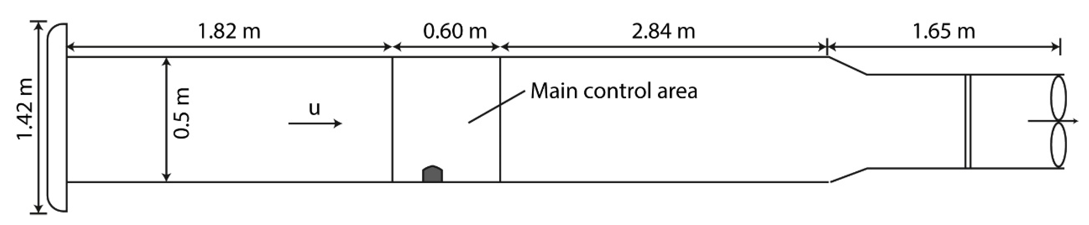
2.1. Wind Tunnel Characteristics

A metal constructed wind tunnel was used in this study (Figure 1). The wind tunnel’s total length was 6.91 m; the cross-section was square with a side length of 0.50 m; and it was previously described in detail in the study of Ntinas et al. [23]. The greenhouse-like obstacle used in this study has an arched roof and has a total height of 0.063 m.

2.2. Mathematical Model

The mathematical simulation was done with the help of modeling using three turbulent models: Standard, RNG and Realizable based on the turbulent k–ε model, which belongs to the commercial package ANSYS FLUENT (ANSYS FLUENT 2021R2, License from the AUTH) [24,25].

Due to the flexibility provided by CFD packages in relation to the “sensitivity analysis” of the problem, it was considered that the best method of analysis would be to configure the model based on the Reynolds number (Re). The value of the Re number determines the type of flow, if it is laminar or turbulent and if it depends on the flow velocity and the geometry of the structure. The Re number was calculated with the formula shown in Equation (1).

$$\mathrm{Re}=\frac{\rho \cdot u\cdot L}{{\mu }^{}}=\frac{u\cdot L}{v}$$

(1)

where:

• ρ: the density of the fluid (kg m⁻³);
• u: flow velocity (m s⁻¹);
• L: the characteristic flow length (m);
• μ: dynamic viscosity (Pa s);
• ν: kinematic viscosity (m² s⁻¹).

For this reason, the transition from laminar to turbulent for each flow type has different critical values of Re number. According to the formula, the Re number depends not only on the velocity, but also on the specific flow length. The specific flow length value is determined by the flow geometry, as mentioned earlier. In many cases, such as in the case of flow in a closed construction, the appropriate characteristic flow length is the diameter of the pipe. It is necessary to point out that, in the present work, the specific flow length, in the calculation of the Re number, is the height of the obstacle: 0.063 m.

Due to the size of the obstacle compared to the size of the wind tunnel, there was no interaction of the boundary layer of the upper wall of the channel with the obstacle. Thus, the main variable parameter of the problem was the velocity of the flow into the tunnel. The logic of this approach has to do with the fact that speed is a factor that directly affects the value of the Re number, which characterizes the type of flow. Each k–ε model was chosen to run at three different inlet airflow velocities (entrance of the wind tunnel) which correspond to three different Re numbers to study meticulously the airflow around a greenhouse (

Table 1. Different inlet airflow velocities for the k–ε models and the corresponding Re numbers.

	Fluent Model	Re	Standard k–ε	RNG k–ε	Realizable k–ε
Velocity (m s−1)
0.34		1364.33	✓	✓	✓
1.00		4012.73	✓	✓	✓
10.00		40127.38	✓	✓	✓

). The three air velocities that were chosen were 0.34, 1.00 and 10.00 m s⁻¹. Consequently, the model ran at all the above speeds, used a constant obstacle height and changed each time the model of k–ε in which it was analyzed. Thus, in the first phase, the respective speeds were analyzed with 3 different approaches represented by the k–ε models (Standard, RNG and Realizable).

During analysis and after the generation of the visualized results of the phenomena that took place around the obstacle, it was found that the area of interest in which noteworthy phenomena occur could be significantly reduced in relation to the total length of the tunnel. Therefore, by running the model each time at a different speed, it was found that the phenomena related to the geometry of the obstacle (mainly turbulence) after a certain distance downstream of the obstacle for the respective air velocity, were so attenuated that were of no interest. Therefore, the control area was limited to only a small section of the long wind tunnel, which was 0.60 m (Figure 2), which resulted in a significant reduction in computing resources and analysis time.

Regarding the type of analysis, it was chosen to be two-dimensional (2D), a choice which is fully justified by the fact that the length of the barrier completely covers the length of the channel (it is supported on the vertical walls of the tunnel). With this assumption, the analysis was simpler and the computational time significantly shorter. Thus, the air passed only over the obstacle, causing in that area any expected detachment phenomena, without the analysis being extended to flows around the obstacle.

The computational setup (inlet, wall treatment, solver, differential schemes) for the present study was as follows:

• Inlet: velocity 0.34, 1, 10 m/s
• Wall treatment: ground, greenhouse line and top of the channel: non-slip condition
• Solver: SIMPLE algorithm was applied
• Outlet: gauge pressure 0
• Differential schemes: Finite Volume Method (FEM)
• In all the models Standard Wall Function was implemented.
• The solution’s convergence criteria were set as follows:
• Continuity: 10-5
• X = velocity: 10-5
• k: 10-5
• ε: 10-5
• No of iterations: 1000

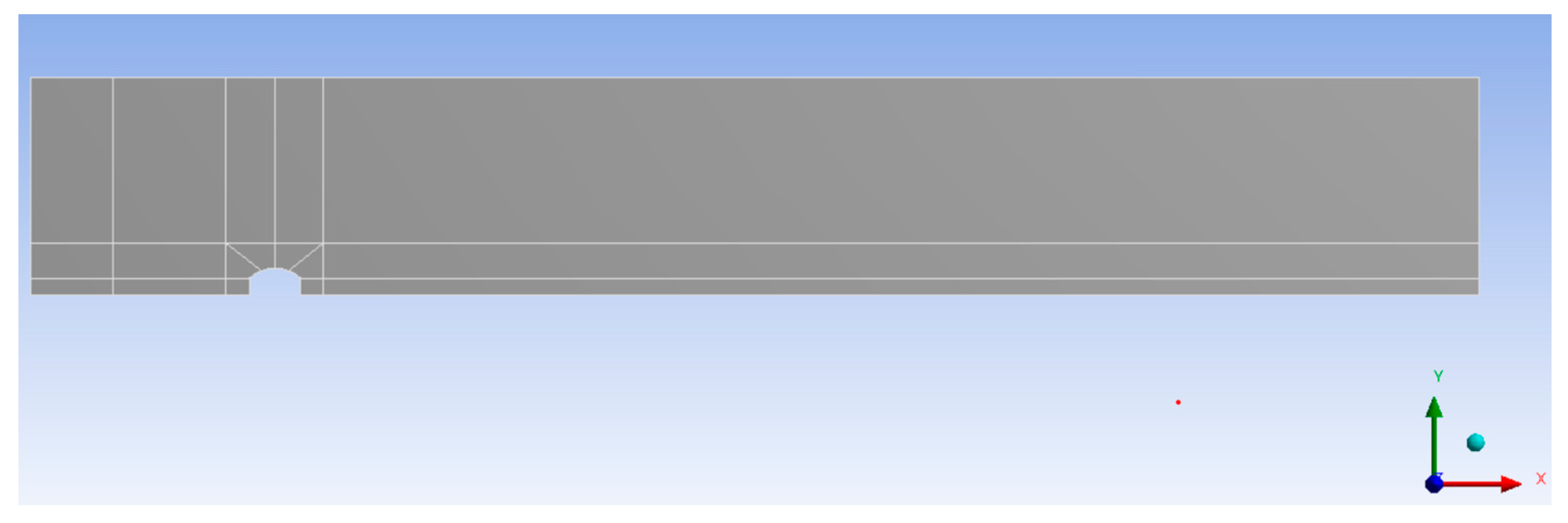
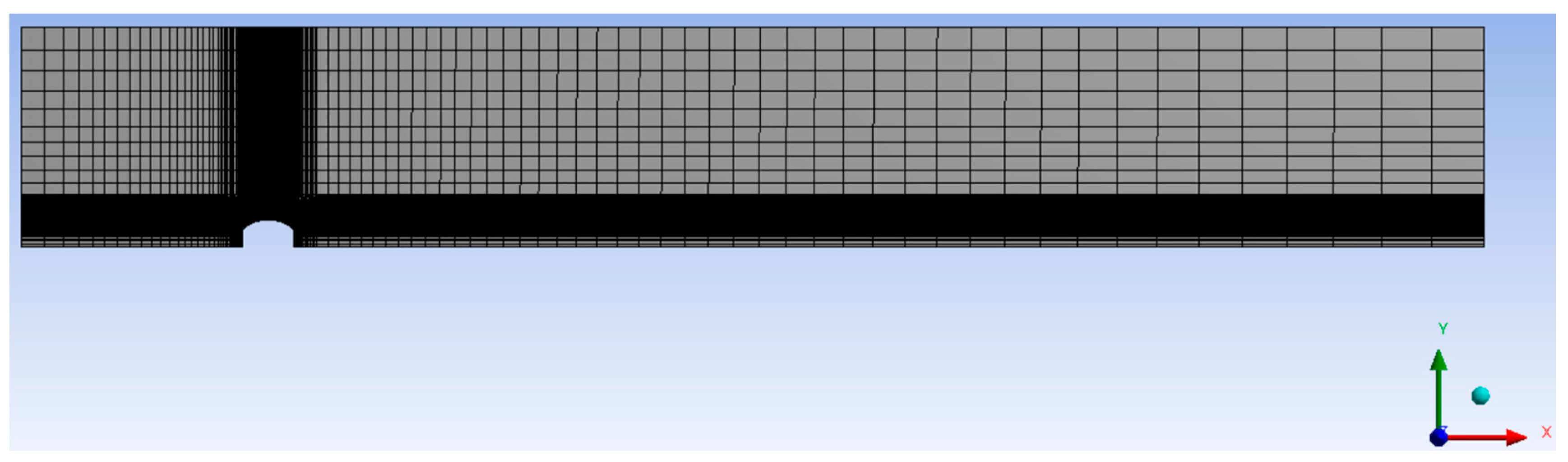
2.3. Computational Mesh

The analysis of the air fluid dynamics behavior over the obstacle involved a series of distinct steps, starting with partitioning the area of the tunnel model under study. It should be emphasized at this point that, as shown in Figure 3, special attention was given to the separation of the area near the obstacle to eliminate problems with the grid development in this area. The turbulent phenomena under investigation were expected to occur mainly in this area. The creation of a well-developed partition of the grid ensured the greatest possible reliability regarding the convergence of solutions in the transmission functions for neighboring data nodes. Otherwise, there was a risk of generating results describing phenomena which do not exist. The nodes numbered 9763, and the elements 9440. Additional thickening of the computer grid showed that it does not affect the solution of the problem.

The next step was the creation of the mesh, and to increase the reliability of the results, suggestions mainly from the user manual of ANSYS FLUENT were considered. Therefore, a grid was constructed with low uniformity, as there were areas of high interest in terms of detachment and turbulent phenomena, while at the same time there were areas where the intensity of the phenomena was negligible. Consequently, in areas of high interest the mesh was significant thickened, and in the rest, there were areas of great distance, and the mesh was more open there (Figure 4).

The blackened area in Figure 4 represents the area of the model in which the density of the mesh was greatly increased. Great importance was given to the area near the obstacle, because it would reveal several phenomena in the flow which were the objects of the present study. For this reason, the area near the greenhouse-like obstacle received the highest density. Accordingly, the mesh around the obstacle area was constructed as shown in Figure 5, and it was done this way to achieve as much speed and pressure data as possible from the areas where intense turbulent phenomena are usually expected (swirls, abrupt changes in the direction of fluid movement due to geometry, etc.). Validation of the models used has been conducted by other researchers using the same experimental air flow conditions as us around modified arched, even rectangular or multi span greenhouses in wind tunnels [8,9], and therefore, it was not the subject of the present work.

3. Results and Discussion

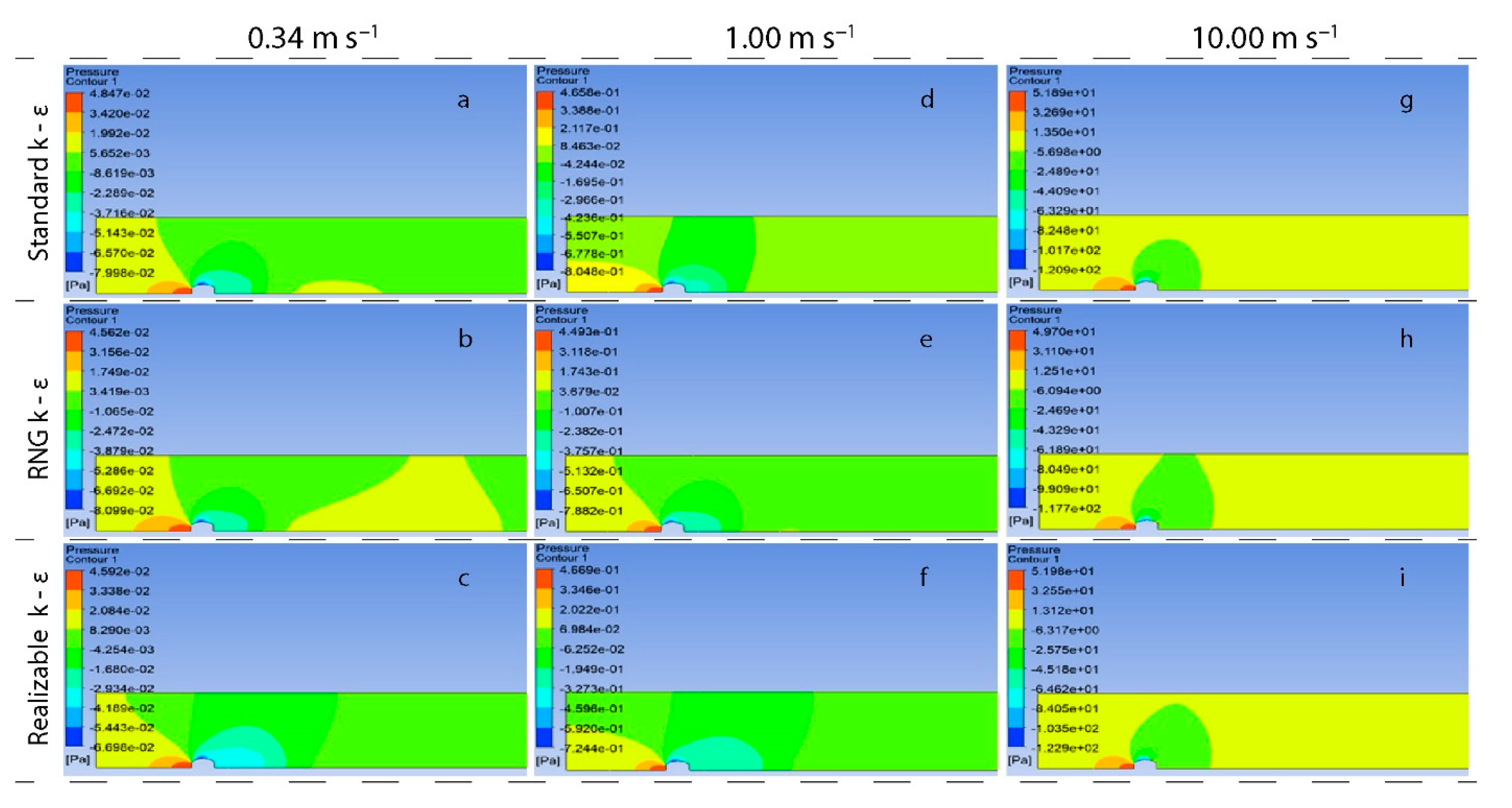
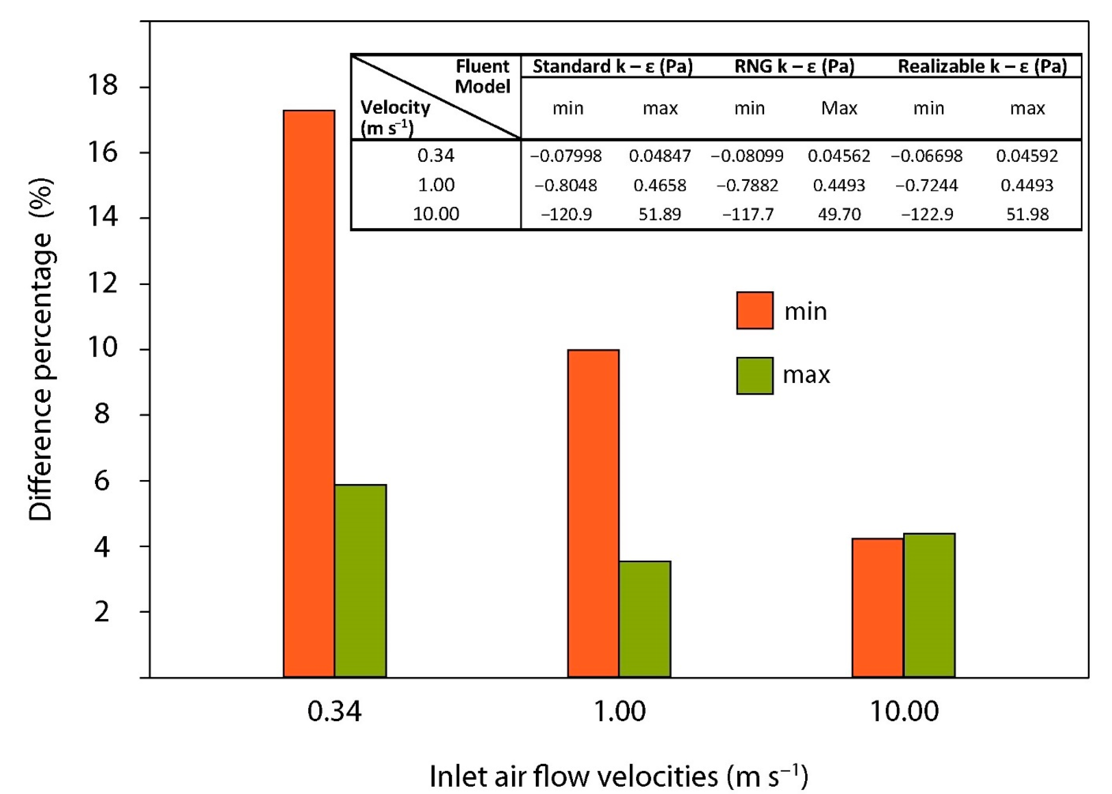
3.1. Pressure Distributions

Pressure distributions were based on the inlet airflow velocities for all available k–ε models (Standard, RNG, Realizable). These velocities were: 0.34, 1.00 and 10.00 m s⁻¹. Figure 6 presents the distributions of pressures developed at the various points of the airflow along the wind tunnel for all the wind velocities under consideration. Negative pressures were observed from the upstream corner of the greenhouse and extended downstream for the cases of inlet airflow velocity of 0.34 and 1.00 m s⁻¹. The same conclusion emerged from the work of Fragos et al. [26] and Kateris et al. [27] for low airflow velocities. In the case of the examined velocity of 10.00 m s⁻¹, a similar distribution was observed, but high negative pressures in absolute values were limited to the roof area of the greenhouse and were more extreme than in those other studies. Upstream of the construction, positive pressure values were observed for all instances of velocities, and they increased as the inlet airflow velocity increased.

The maximum differences in the pressure values which resulted from the modeling of the problem and between the k–ε models appeared in the case of the minimum values of the displayed manometric pressure. This difference narrowed impressively as the mainstream speed increased. The maximum difference in pressure values between the k–ε models reached 17% when the air velocity was set to 0.34 m s⁻¹. The corresponding difference was 4% in the case of 10.00 m s⁻¹ air velocity (Figure 7). The same trend appeared in the convergence of the maximum displayed pressure values, although admittedly the deviations between the k–ε models for the respective flow rate were significantly smaller. The differences in pressure values between the models decreased as the value in the fluid flow rate increased, as presented in Figure 7.

Τhe positions of the maximum and the minimum pressure in all the models and for the three velocities set, are almost in the same places of the wind tunnel. The maximum pressure was in front of the obstacle, something that was expected, as at this point the speed must be zero (Figure 6). Furthermore, the minimum pressure value appeared on the curvature of the obstacle’s roof just before its highest point. Although the positions of the maximum and minimum pressure values in all models were similar, the pressure distributions for the same flow velocity throughout the wind tunnel appeared to be more similar among cases with higher flow velocities (10.00 m s⁻¹) than cases with lower ones. This observation combined with the fact that the percentage differences in pressure values decreased as the flow rate increased, led to the first conclusion that the results from the three k–ε models (Standard, RNG, Realizable) start and converge as the flow rate increases.

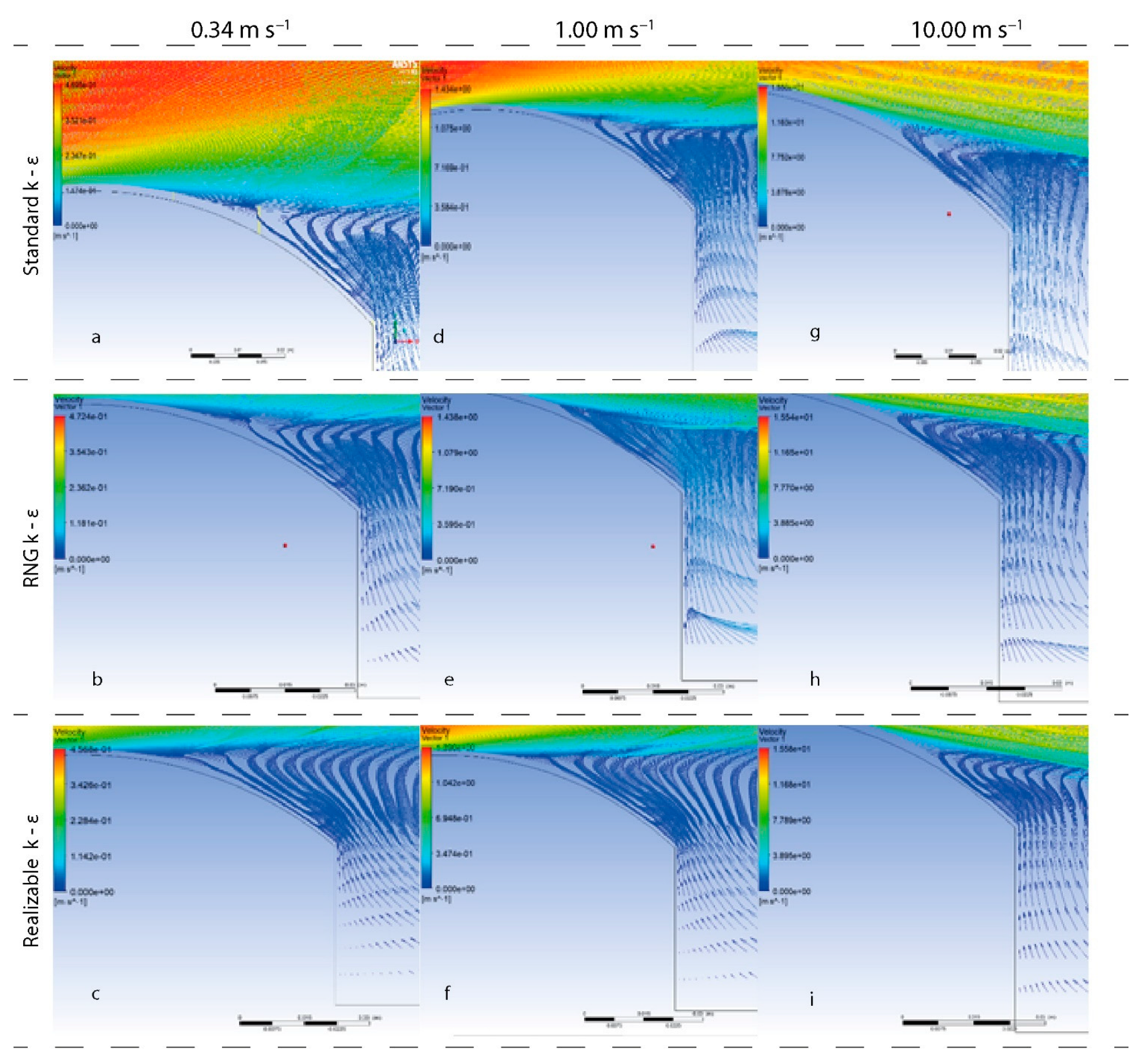
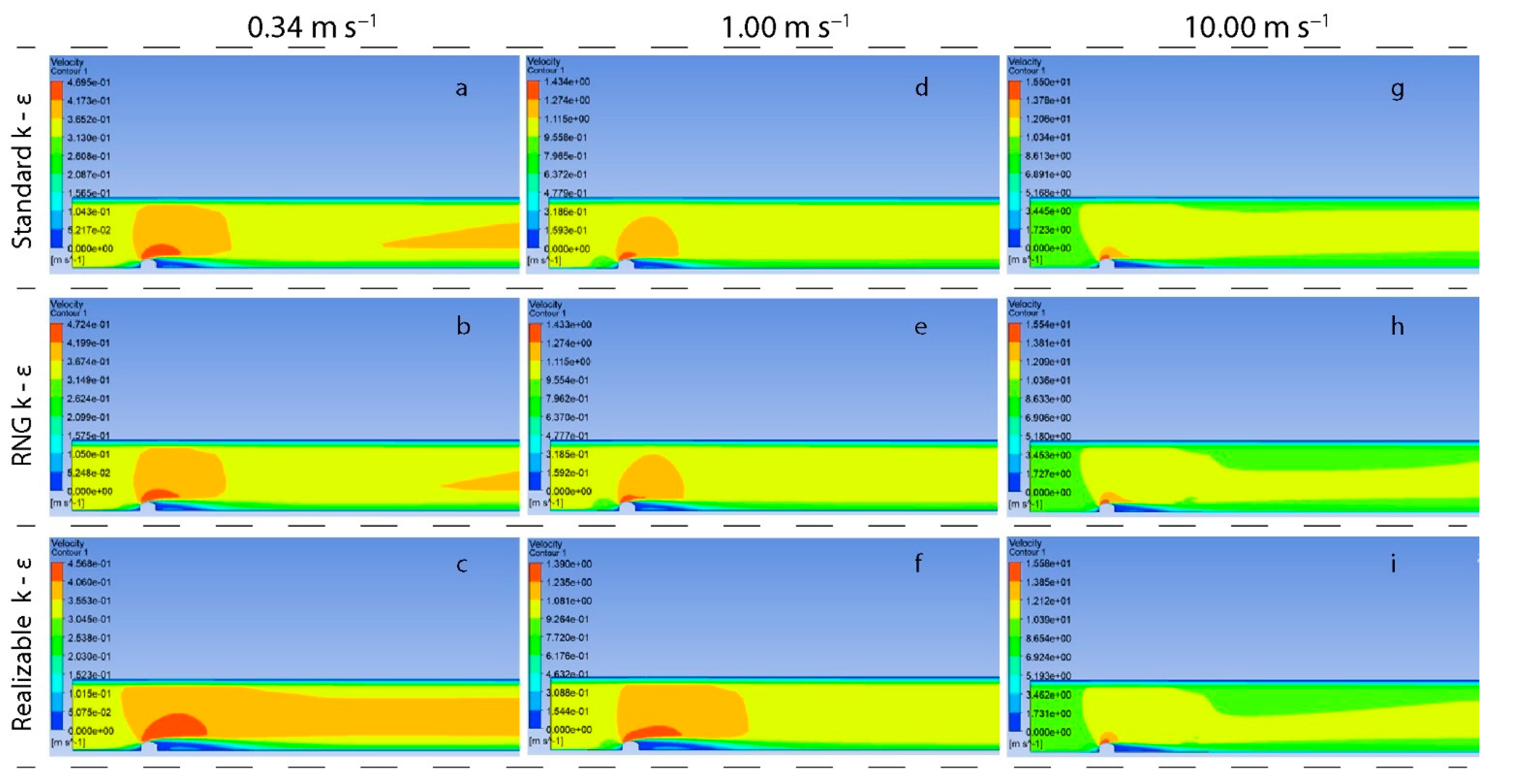
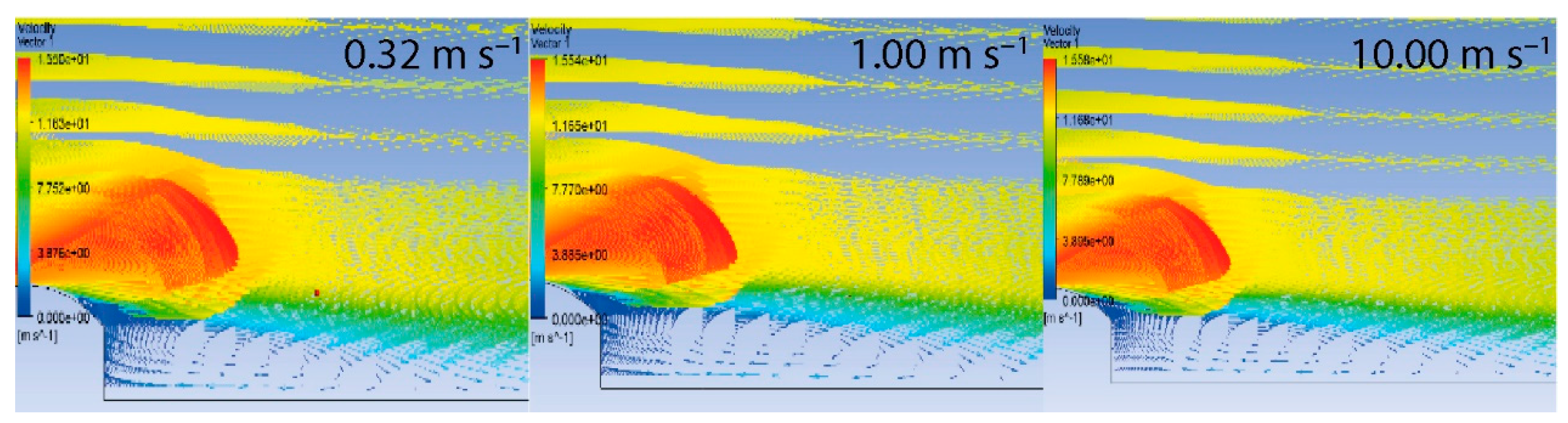
3.2. Air Velocity Distributions

Following the pattern adopted for the pressure distributions of the previous section, the air velocity distributions are studied here. The results that are analyzed are presented in Figure 8, Figure 9 and Figure 10.

The maximum values of the velocities along the airflow in the wind tunnel and the speed differences (%) between the models for the different air speed velocities are presented in Figure 10. When the flow velocity increases, so does the convergence of the results of the three k–ε models, in terms of pressure and velocity within the wind tunnel, as can be seen in Figure 9. The percentage of surface area at which high speeds are predicted also signifies the qualitative differences in the speed distributions. When the velocity was 0.34 m s⁻¹, the Realizable model predicted that the speed will be up to 20% higher at almost 75% of the wind tunnel. As expected, all models predicted that the maximum speed would be on the roof of the model (Figure 8 and Figure 9).

However, it should be noted that the area in which the upper speed limit appears decreases for all three models (Standard, RNG, Realizable) as the flow velocity increases. In fact, when the flow velocity was set to 10 m s⁻¹, the area where the upper speed limit appears could be found only above the obstacle (Figure 9).

By analyzing the values of the maximum displayed velocities for each model, considering the flow velocity as a parameter, Figure 10 was obtained, which shows the maximum differences in the velocity values between the models for the same flow velocities and the maximum air velocities obtained inside the wind tunnel by all k–ε models.

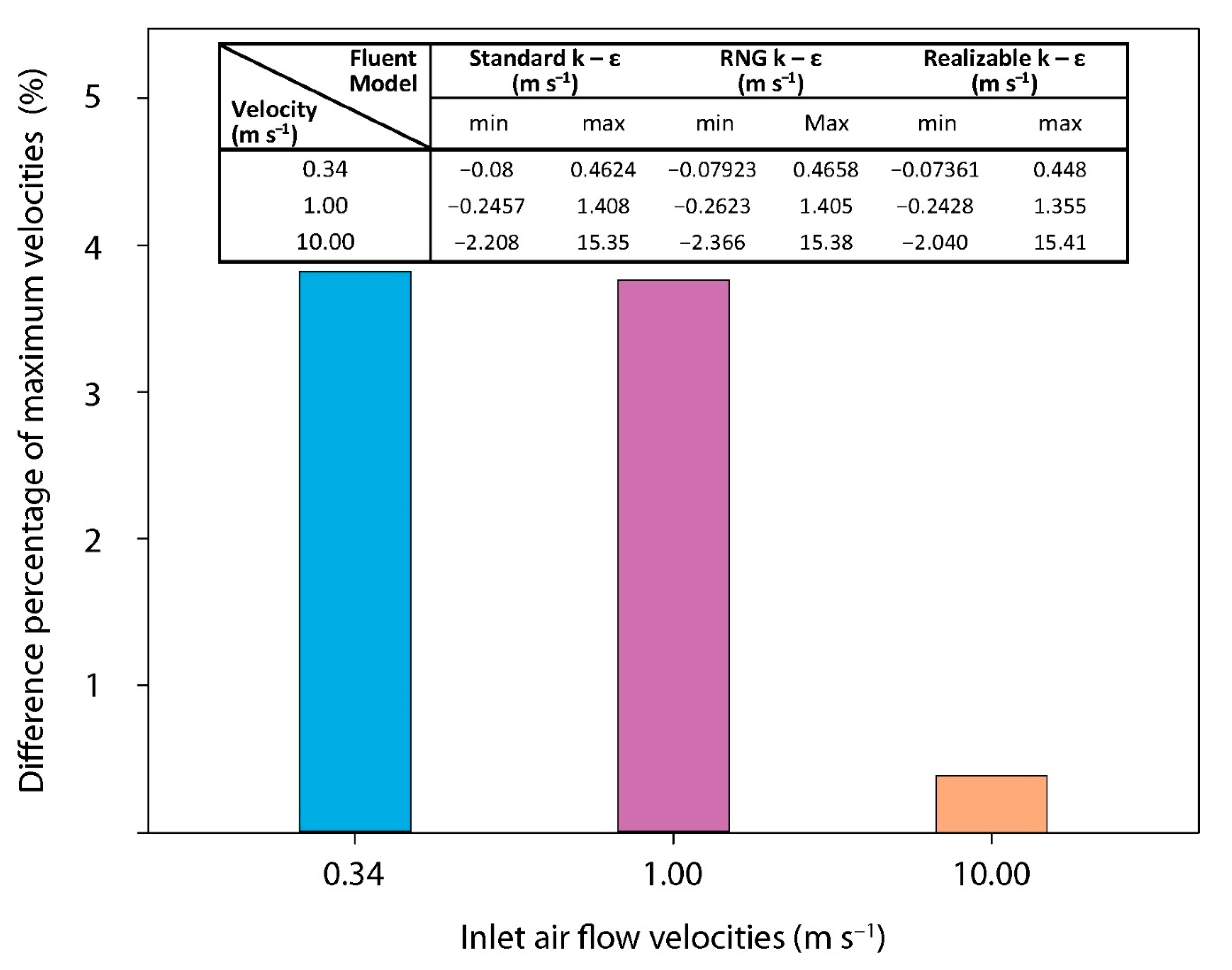
3.3. Horizontal Speed Distributions (u)

The velocities shown in Figure 8 and Figure 9 and analyzed in the previous section had a minimum value of zero. This could lead to the erroneous conclusion that there was no negative velocity on the obstacle, resulting in the absence of inverted flow. This was the main reason why the analysis proceeded further to investigate the speed distributions on the horizontal plane (u).

At this point, it should be clarified that the velocity analyzed in the previous section was the vector sum of the two perpendicular velocity components (u and v). The measure of this velocity (which is always positive) is given by the well-known Pythagorean theorem:

$$U=\sqrt{u^2+v^2}$$

(2)

Figure 11 shows the horizontal velocity distributions for all velocity cases and for all k–ε models. Inverted flow accounted for 20–26% of the inlet airflow velocity in the wind tunnel in all models. The area of maximum values using all models was above the obstacle, as found in other studies [4,23], but was limited as the air entry velocity into the wind tunnel increased. The recirculation length of the flow downstream of the obstacle, as shown by the horizontal velocity distribution, decreased as the flow increased. The numerical approximation of the recirculation length does not appear to be affected by the model used in cases of high velocity. The horizontal velocity distribution confirms that the convergence between the various k–ε models in terms of velocities increased when the inlet airflow velocity of the wind tunnel increased.

Figure 12 presents the maximum percentage differences in u_max among the k–ε models for the inlet airflow velocities of 0.34, 1.00 and 10.00 m s⁻¹ respectively; and the maximum and minimum of horizontal velocities (m s⁻¹) in the wind tunnel for all models. As can be seen in Figure 12, the smallest d between the Standard, RNG, and Realizable models (0.4%) occurred for the highest flow rate (10 m s⁻¹). The maximum and minimum values of wind velocity had significant effects on the structural characteristics of the flow, and the minimum values influenced the efficiency and the design of the natural ventilation of the greenhouses. Natural ventilation is one of the basic environmental control techniques for the proper growth of the plants in greenhouses. The design of a greenhouse requires meticulously study of natural ventilation (dimensions of roof and side openings, ventilation rate, etc.) and the climate of the area where it is going to be established.

Figure 13 shows the vector illustrations of the presence or absence of vortices in the area before the obstacle. The results refer to velocity and pressure profiles only of the Standard model k–ε for the three airflow entry velocities in the wind tunnel where each model was studied. This approach was chosen because the respective profiles from the RNG and Realizable models did not differ in terms of the quality of their results from the Standard k–ε model.

The existence of clockwise vortices for the airflow entry velocities of 0.34 and 1.00 m s⁻¹ into the wind tunnel is shown in Figure 14. Obvious vortices in the case of 10 m s⁻¹ are missing (Figure 14). In this case, it could be explained that as the flow velocity of the model increased, the vortex was pressed against the wall, thereby decreasing in size.

Figure 14 shows the inverted flow over the right end of the obstacle for the three airflow entry velocities studied. The results concern the vector analysis that resulted from the solution of the k–ε Standard model, for the same reason mentioned previously. The analysis of the figure indicates that there was reverse flow between the main flow and the right half of the obstacle roof for all flow velocities. To complete the downstream analysis of the obstacle area, the vector representations of the downstream flows around the greenhouse from the solutions of the Standard k–ε model for the three airflow entry velocities studied are presented in Figure 15. The development of an almost elliptical swirl is evident in the area directly after the obstacle, regardless of the air entry velocity into the wind tunnel.

4. Conclusions

In this study, an attempt was made to model the airflow over an obstacle of a greenhouse-like shape located inside an air tunnel, by using the commercial package ANSYS FLUENT. The extant possibilities of modeling through FLUENT allowed us to conduct an in-depth investigation of the airflow through analysis of velocity and pressure profiles. Several conclusions were drawn from the analysis of the results, and the most important can be mentioned as follows:

• The results of k–ε models for pressure and velocity converged when the velocity of the air was high enough to ensure that the flow was turbulent. The results showed that the three models converge significantly when the inlet air velocity reaches 10 m/s, and thus all three models are suitable for this air velocity value.
• The presence of turbulence in the flow can be diagnosed by analyzing the airflow velocity profiles. The horizontal velocity profile has a key role in this investigation.
• For a greenhouse with an arched roof, there are three areas in which vortices develop. These are upstream, above the roof and downstream.
• As the flow velocity increases, the magnitude of the vortex upstream of the obstacle decreases, resulting in its elimination at very high velocities.
• The vortex that appears on the roof of the obstacle is an extension of the vortex created downstream of the obstacle.

The evolution of computational technology allows the study of complex flows using remarkable commercial computing packages that solve turbulent models and offer the possibility for a more realistic approach to such flows by directly solving the Navier–Stokes equations with direct numerical simulations.

References

1. Bartzanas, T.; Kittas, C.; Sapounas, A.A.; Nikita-Martzopoulou, C. Analysis of airflow through experimental rural buildings: Sensitivity to turbulence models. Biosyst. Eng. 2007, 97, 229–239. [Google Scholar] [CrossRef]
2. Norton, T.; Grant, J.; Fallon, R.; Sun, D.W. Improving the representation of thermal boundary conditions of livestock during CFD modeling of the indoor environment. Comput. Electron. Agric. 2010, 73, 17–36. [Google Scholar] [CrossRef]
3. Shen, X.; Zhang, G.; Bjerg, B. Comparison of different methods for estimating ventilation rates through wind driven ventilated buildings. Energy Build. 2012, 23, 297–306. [Google Scholar] [CrossRef]
4. Vogiatzis, I.; Denizopoulou, A.C.; Ntinas, G.K.; Fragos, V.P. Simulation analysis of air flow and turbulence statistics in a rib grit roughened duct. Sci. World J. 2014, 2014, 791513. [Google Scholar] [CrossRef]
5. Ntinas, G.K.; Denizopoulou, A.C.; Kotsopoulos, T.A.; Fragos, V.P. Numerical Approximation of Airflow inside an Agricultural Structure. Sci. Technol. Built Environ. Sci. Technol. Built Environ. 2017, 23, 382–390. [Google Scholar] [CrossRef]
6. Ntinas, G.K.; Dados, N.J.; Shen, X.; Malamataris, N.; Fragos, V.P.; Zhang, G. Characteristics of unsteady flow around two successive rectangular ribs on floor of a wind tunnel. Eur. J. Mech. –B/Fluids 2017, 63, 450–458. [Google Scholar] [CrossRef]
7. Norton, T.; Sun, D.W.; Grant, J.; Fallon, R.; Dodd, V. Applications of computational fluid dynamics (CFD) in the modelling and design of ventilation systems in the agricultural industry: A review. Bioresour. Technol. 2007, 98, 2386–2414. [Google Scholar] [CrossRef]
8. Ntinas, G.K.; Shen, X.; Wang, Y.; Zhang, G. Evaluation of CFD turbulence models for simulating external airflow around varied building roof with wind tunnel experiment. Build. Simul. 2018, 11, 115–123. [Google Scholar] [CrossRef]
9. Kim, R.W.; Lee, I.B.; Kwon, K.S. Evaluation of wind pressure acting on multi-span greenhouses using CFD technique, Part 1: Development of the CFD model. Biosyst. Eng. 2017, 164, 235–256. [Google Scholar] [CrossRef]
10. Kuroyanagi, T. Investigating air leakage and wind pressure coefficients of single-span plastic greenhouses using computational fluid dynamics. Biosyst. Eng. 2017, 163, 15–27. [Google Scholar] [CrossRef]
11. Akrami, M.; Javadi, A.A.; Hassanein, M.J.; Farmani, R.; Dibaj, M.; Tabor, G.R.; Negm, A. Study of the effects of vent configuration on mono-span greenhouse ventilation using computational fluid dynamics. Sustainability 2020, 12, 986. [Google Scholar] [CrossRef] [Green Version]
12. Roache, P.J. Perspective: A method for uniform reporting of grid refinement studies. J. Fluids Eng. Trans. ASME 1994, 116, 405–413. [Google Scholar] [CrossRef]
13. Murakami, S. Comparison of various turbulence models applied to a bluff body. J. Wind Eng. Ind. Aerodyn. 1993, 46-47, 21–36. [Google Scholar] [CrossRef]
14. Murakami, S. Overview of turbulence models in CWE—1997. J. Wind Eng. Ind. Aerodyn. 1998, 74–76, 1–24. [Google Scholar] [CrossRef]
15. Molina-Aiz, F.D.; Valera, D.L.; Álvarez, A.J. Measurement and simulation of climate inside Almeria—Type greenhouses using computational fluid dynamics. Agric. For. Meteorol. 2004, 125, 33–51. [Google Scholar] [CrossRef]
16. Ould Khaoua, S.A.; Bournet, P.E.; Migeon, C.; Boulard, T.; Chasseriaux, G. Analysis of greenhouse ventilation efficiency based on computational fluid dynamics. Biosyst. Eng. 2006, 95, 83–89. [Google Scholar] [CrossRef]
17. Casey, M.; Wintergerste, T. Best Practice Guidelines ERCOFTAC Special Interest Group on Quality and Trust in Industrial CFD. ERCOFTAC 2000. Available online: https://www.ercoftac.org/downloads/watermarks/not_in_use/bpg_spf_version_1.pdf (accessed on 20 May 2021).
18. Tominaga, Y.; Mochida, A.; Yoshie, R.; Kataoka, H.; Nozu, T.; Yoshikawa, M.; Shirasawa, T. AIJ guidelines for practical applications of CFD to pedestrian wind environment around buildings. J. Wind Eng. Ind. Aerodyn. 2008, 96, 1749–1761. [Google Scholar] [CrossRef]
19. Blocken, B. 50 years of Computational Wind Engineering: Past, present and future. J. Wind Eng. Ind. Aerodyn. 2014, 129, 69–102. [Google Scholar] [CrossRef]
20. Gholami, A.; Bonakdari, H.; Zaji, A.H.; Akhtari, A.A. Simulation of open channel bend characteristics using computational fluid dynamics and artificial neural networks. Eng. Appl. Comput. Fluid Mech. 2015, 9, 355–369. [Google Scholar] [CrossRef]
21. Dai, X.; Liu, J.; Zhang, X. A review of studies applying machine learning models to predict occupancy and window-opening behaviours in smart buildings. Energy Build. 2020, 223, 110159. [Google Scholar] [CrossRef]
22. Moradzadeh, A.; Mohammadi-Ivatloo, B.; Abapour, M.; Anvari-Moghaddam, A.; Roy, S.S. Heating and Cooling Loads Forecasting for Residential Buildings Based on Hybrid Machine Learning Applications: A Comprehensive Review and Comparative Analysis. IEEE Access 2022, 10, 2196–2215. [Google Scholar] [CrossRef]
23. Ntinas, G.K.; Zhang, G.; Fragos, V.P.; Bochtis, D.D.; Nikita-Martzopoulou, C. Airflow patterns around obstacles with arched and pitched roofs: Wind tunnel measurements and direct simulation. Eur. J. Mech.-B/Fluids 2014, 43, 216–229. [Google Scholar] [CrossRef]
24. Yakhot, V.S.A.S.T.B.C.G.; Orszag, S.A.; Thangam, S.; Gatski, T.B.; Speziale, C. Development of turbulence models for shear flows by a double expansion technique. Phys. Fluids A Fluid Dyn. 1992, 4, 1510–1520. [Google Scholar] [CrossRef] [Green Version]
25. Launder, B.E.; Spalding, D.B. The numerical computation of turbulent flows. Comput. Methods Appl. Mech. Eng. 1974, 3, 269–289. [Google Scholar] [CrossRef]
26. Fragos, V.P.; Ntinas, G.K.; Kateris, D.L. Numerical estimation of external pressure coefficients of a pitched—Type roof greenhouse and comparison with Eurocode in different flow—Type circumstances. In Proceedings of the International Conference of Agricultural Engineering, Zurich, Switzerland, 6–10 July 2014; pp. 1–7. [Google Scholar]
27. Kateris, D.L.; Fragos, V.P.; Kotsopoulos, T.A.; Martzopoulou, A.G.; Moshou, D. Calculated external pressure coefficients on livestock buildings and comparison with Eurocode 1. Wind Struct. 2012, 15, 481–494. [Google Scholar] [CrossRef]
Figure 1. Wind tunnel scheme and basic dimensions.
Agriengineering 04 00016 g001
Figure 2. Position of the located main control area in the wind tunnel.
Agriengineering 04 00016 g002
Figure 3. Partitioning of the wind tunnel.
Agriengineering 04 00016 g003
Figure 4. Computational mesh of the wind tunnel.
Agriengineering 04 00016 g004
Figure 5. The computational mesh near the greenhouse-like obstacle.
Agriengineering 04 00016 g005
Figure 6. Pressure distributions for the wind tunnel flow velocities of 0.34, 1.00 and 10.00 m s−1 from Standard k–ε (a,d,g), RNG k–ε (b,e,h) and Realizable k–ε (c,f,i) models.
Agriengineering 04 00016 g006
Figure 7. The highest percentage differences in the pressure values in relation to the flow velocity and the maximum and minimum pressure values (Pa) in the wind tunnel for all models.
Agriengineering 04 00016 g007
Figure 8. The vector representations for the wind tunnel flow velocities of 0.34, 1.00 and 10.00 m s−1 using Standard k–ε (a,d,g), RNG k–ε (b,e,h) and Realizable k–ε (c,f,i) models.
Agriengineering 04 00016 g008
Figure 9. Air velocity distributions for the wind tunnel flow velocities of 0.34, 1.00 and 10.00 m s−1 using Standard k–ε (a,d,g), RNG k–ε (b,e,h) and Realizable k–ε (c,f,i) models.
Agriengineering 04 00016 g009
Figure 10. Maximum speed differences between models for the selected flow velocities (%) and the maximum air speeds (m s−1) in the wind tunnel from all the examined models.
Agriengineering 04 00016 g010
Figure 11. Air velocity (u) distribution for the wind tunnel flow velocities of 0.34, 1.00 and 10.00 m s−1 from Standard k–ε (a,d,g), RNG k–ε (b,e,h) and Realizable k–ε (c,f,i) models.
Agriengineering 04 00016 g011
Figure 12. The maximum percentage differences in umax among the k–ε models for the inlet airflow velocities of 0.34, 1.00 and 10.00 m s−1 respectively; and the maximum and minimum of horizontal velocities (m s−1) in the wind tunnel for all models.
Agriengineering 04 00016 g012
Figure 13. The vector illustrations of the upstream flow of the obstacle from the solution of the Standard k–ε model for 0.32, 1.00 and 10.00 m s−1 airflow entry into the wind tunnel velocities.
Agriengineering 04 00016 g013
Figure 14. The inversion of the flow at the end of the structure from the solutions of the Standard k–ε model for 0.32, 1.00 and 10.00 m s−1 airflow entry velocities into the wind tunnel.
Agriengineering 04 00016 g014
Figure 15. The vector illustrations of the downstream flow of the obstacle from the solutions of the Standard k–ε model for 0.32, 1.00 and 10.00 m s−1 airflow entry into the wind tunnel velocities.
Agriengineering 04 00016 g015