Abstract
UAV may be limited by its flight height and camera resolution when aerial photography of a tea garden is carried out. The images of the tea garden contain trees and weeds whose vegetation information is similar to tea tree, which will affect tea tree extraction for further agricultural analysis. In order to obtain a high-definition large field-of-view tea garden image that contains tea tree targets, this paper (1) searches for the suture line based on the graph cut method in the image stitching technology; (2) improves the energy function to realize the image stitching of the tea garden; and (3) builds a feature vector to accurately extract tea tree vegetation information and remove unnecessary variables, such as trees and weeds. By comparing this with the manual extraction, the algorithm in this paper can effectively distinguish and eliminate most of the interference information. The IOU in a single mosaic image was more than 80% and the omissions account was 10%. The extraction results in accuracies that range from 84.91% to 93.82% at the different height levels (30 m, 60 m and 100 m height) of single images. Tea tree extraction accuracy rates in the mosaic images are 84.96% at a height of 30 m, and 79.94% at a height of 60 m.
1. Introduction
UAV has been widely used in agricultural irrigation, farmland vegetation data monitoring, soil temperature monitoring, agricultural disaster monitoring or evaluation, and site exploration due to its advantages of high time-efficiency, low loss, high resolution, and low cost [1,2]. UAVs can carry different kinds of cameras to obtain aerial images at different altitudes according to the different requirements. They can also carry out relevant processing on the captured images [3,4] to obtain required parameters and information [5,6]. However, limited by altitude and camera resolution, it is difficult to obtain a wide range of high-definition images, especially in agriculture or forestry. A single image only contains local information if the target area and crop distribution are large, such as a tea garden.
Image mosaic technology has been widely studied in many fields to stitch the images together. It includes image registration and image fusion. The image registration results affect the image fusion. With the diversity of the actual scenes, it is difficult to design a registration algorithm suitable for all scenes. To date, image registration includes frequency-based image registration and space-based image registration. Frequency-based image registration uses the Fourier transform to transform the image to the frequency domain for related processing. The typical frequency-based image registration is the Fourier–Mellin transform [7], phase correlation method [8] and the extended phase correlation method [9]. According to the research, it is known that frequency-based image registration methods can overcome the brightness difference and anti-noise and it is fast and efficient. However, it requires a large overlap ratio between two images, which is mainly applied to the horizontal transformation [10,11]. Therefore, the use of this method in a tea garden is greatly limited. The space-based image registration method is based on gray level or images features. The former divides the overlapping areas of one image into multiple sub areas and calculates their similarity of pixel values using a certain similarity criterion to obtain the translation. The principle of this algorithm is simple. Meanwhile, the registration effect of rigid transformation is good. However, it is greatly affected by illumination and noise, resulting in a large number of calculations [12]. To date, image registration based on features is the most widely used [12,13]. The features generally include feature points, straight lines, edges, and contours. This kind of registration algorithm extracts and matches the corresponding feature points of two images. Then, it calculates the transformation model between the two images to complete the registration.
Vegetation research has great potential in crop management. To date, most vegetation research is based on the information collected from multispectral or hyperspectral data for related processing, and the relevant parameters are reverse-performed based on the information in the visible and near-infrared bands [14]. Summer et al. used hyperspectral remote sensing to retrieve the winter wheat leaf area index (LAI) to evaluate its growth and predict its yield. Spectral indexes are used to extract leaf chlorophyll content for analysis and evaluation [15,16]. For images in the visible light bands, common indexes include ultra-green index Exg [17] and the normalized green-red difference index NGRDI [18]. Torres et al. [19] and Rasmussen et al. [20] calculated the visible vegetation index to study crop coverage. Researchers [21,22] achieved the extraction of tree information through tree point cloud data generated by airborne LIDAR and contour fitting. However, there are relatively few studies on the differentiation of the varieties of green vegetation.
If the UAVs cannot obtain a wide range of high-definition images of agriculture and forestry simultaneously, the information of each single image is limited, particularly when the planting area is large, or the crop distribution is not regular, such as in large tea gardens in China. The subsequent analysis of the images becomes complex and results in limitations. By using image mosaic technology, we can obtain comprehensive information about the whole tea garden. Meanwhile, it is a more flexible method to capture images. After the mosaics of the images, it is more conducive for further vegetation analysis. It can also be combined with remote sensing technology to monitor the crop growth and perform disaster assessments in precision agriculture [23]. The complexity of tea gardens results in difficulties of the analysis of tea trees [24]; aerial images of tea gardens usually contain similar vegetation information of tea trees, such as weeds and other green crops [25]. In order to solve the target extraction problem caused by the limitation of the flight height in mosaic images of tea gardens, we (1) captured tea garden images at three different heights; (2) improved the energy function to search the suture line of mosaic tea garden images; and (3) built a feature vector to extract the tea trees from mosaiced images. This paper discusses the effects of the different heights on tea garden image mosaicking and tea tree extraction. The findings provide a robust method for image mosaicking, especially for tea gardens and tea tree target extraction.
2. Materials and Methods
2.1. Data Collection
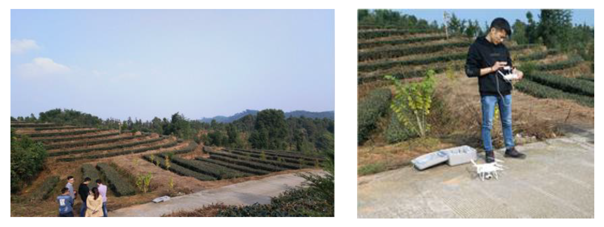
The tea garden images in this paper were all obtained from a tea garden experimental field (Figure 1) located in Yanshan, Yinbin, Sichuan, China (104°667′ W, 28°915′ N). The test area is about 9 mu, with an average altitude of about 530 m. The drone (Phantom 3SE, DJI, Shenzhen, China) was controlled by a trained drone operator from the Yibin Agricultural Machinery Institute. First, the operator used a remote controller to control the drone to fly to the desired area. Then, he adjusted the drone at the certain heights (30, 60, 100 m in the study). Finally, he stopped moving the drone and took the pictures in a relatively stationary state in the air. All the images were manually taken using a camera (1 inch CMOS, FOV: 77°, equivalent focal length: 28 mm, f/2.8–f/11, autofocus, electronic shutter: 8 to 1/8000 s) on the drone. The day we conducted the experiment was cloudy and the light was relatively stable.
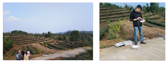
Figure 1.
Photograph of the tea garden and the drone operator.
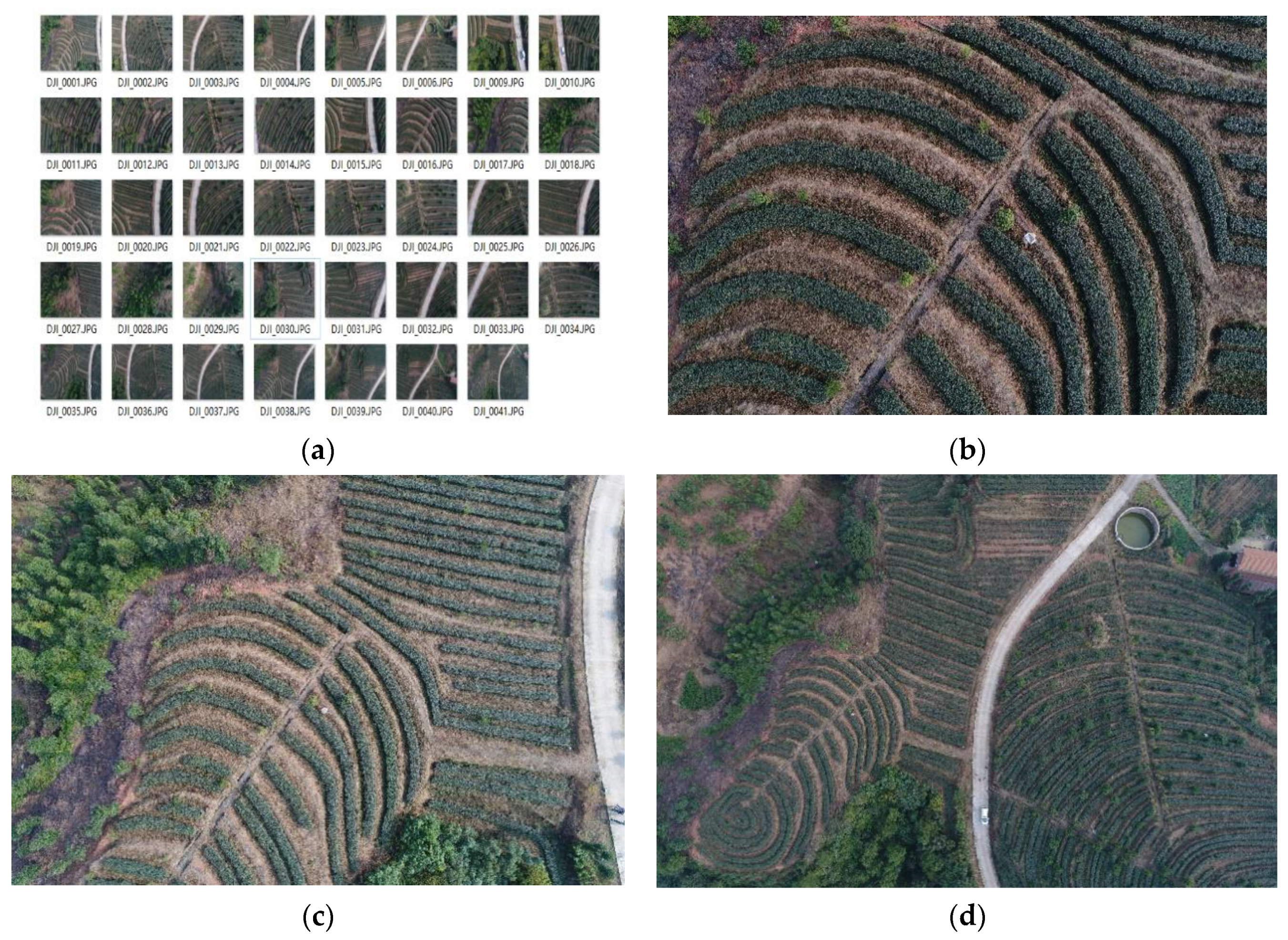
Raw image datasets of the tea garden are shown in Figure 2. The tea garden images contain three groups of RGB images of different heights. “Group 1”(Figure 2b) contains 34 images from 30 m high with a GSD (ground sample distance) of 0.53 cm; “Group 2” (Figure 2c) contains 6 images from 60 m high with a GSD of 1.07 cm; and “Group 3” (Figure 2d) contains 1 image from 100 m high with a GSD of 1.78 cm. The images of Group 1 and Group 2 were used for image mosaicking, of which the results will be compared with Group 3.

Figure 2.
Raw image datasets of the tea garden. (a) Images of the tea garden dataset; (b) one image from 30 m high (“Group 1”); (c) one image from 60 m high (“Group 2”); (d) the image from 100 m high (“Group 3”).
2.2. Image Preprocessing
2.2.1. Image Denoising
In the process of image collection, it is inevitably affected by the equipment, environment, and other factors that create image noises. These noises reduce the stitching quality. In this study, we used a Gauss filter to decrease the noises.
2.2.2. Distortion Correction
In general imaging, the deviation of lens manufacturing precision and assembly process leads to distortion, resulting in the final image registration. Geometric distortion also has a certain impact on image registration, causing the matched points to not match successfully in the end, so it is necessary to build a distortion model to transform the image to eliminate this impact.
2.3. Image Registration Based on Feature Point Extraction
2.3.1. Feature Point Extraction
The SIFT (scale invariant feature transform) algorithm [26] is a classical scale invariant algorithm with an invariability of scale and rotation and good robustness for illumination and angle transformation. In this space, the extreme values are found, feature points are located, direction is determined and descriptors are constructed concerning the selected neighborhood. The SIFT algorithm process is described below.
- (1)
- Construct a Gaussian difference pyramid.
Firstly, the original image was Gaussian filtered. The variance of continuous variation was used to obtain a group of images that were the same size as the original image. The whole process can be expressed in the following Formula (1):
where represents the raw image, and represent the coordinates of the image pixels, the Gaussian kernel is generally abbreviated as , , and represents the variance, also known as the scale.
After the above operations, a scale space was obtained for the image with the same resolution, and the blur degree of the image in the scale space increased gradually. In order to ensure the continuity of the scale space, the penultimate image of the previous layer is usually sampled twice and the image obtained is used as the initial image of the next step. Then, the steps above were repeated many times to obtain multiple scale spaces. The multilayer image from top to bottom, from small to large, were arranged in a shape similar to a pyramid, the so-called the Gauss pyramid. In this study, we used , indicates the number of layers required to obtain the Gaussian pyramid.
Then, N pairs of images in each layer were subtracted from the adjacent two pairs of images to obtain n − 1 pairs of difference images shown Formula (2):
- (2)
- Locating and screening key points.
In each layer of the pyramid, two boundary images were removed. Each one of them has two adjacent images. In the 3D space, each point has 26 neighborhood points. By comparing them, the maximum or minimum value was retained in order to find the most stable points, which are the discrete points in the space. In order to improve the stability of the key points, curve interpolation is needed for the scale space, and the Taylor expansion of the differential scale space is represented by Formula (3):
Taking the derivative of and setting the equation to zero produces the offset of the extreme point. Assume that is the offset shown in Formula (4):
If the value is greater than 0.5, the interpolation center has shifted to the adjacent point. Therefore, the location of the current key point must be changed and iterations must be repeated to convergence. In this paper, we set a threshold value of 0.03. When , directly eliminate the contrast at a low point. In this process, the exact position and scale ∂ of the extreme point are obtained in Formula (5):
- (3)
- Build feature descriptors.
The scale space is used to allow the feature points obtain a certain scale invariance. In order to ensure the rotation invariance and facilitate the registration of subsequent feature points, a unique descriptor is usually calculated for each feature point according to its neighborhood.
First, the main direction of the feature points should be determined. According to the second step, the gradient and direction distribution of all pixels in the 3σ neighborhood window on the Gaussian image closest to the feature point are determined, and the gradient histogram is constructed. In order to prevent interference in one direction, Gaussian smoothing is also needed. The gradient and the direction in the neighborhood of the feature point are calculated by the Formulas (6) and (7):
After the main directions of the key points are calculated, descriptors of the feature points are constructed according to the main directions. For it to obtain rotation invariance, its coordinates first need to be rotated in the main direction. Then, the direction in the neighborhood is calculated with the feature point as the center and the main direction as the reference coordinate. In the original text, the 16 × 16 pixels of the neighborhood were calculated, and a seed point was formed for every 4 × 4 pixels, and the size in 8 directions in each seed region was calculated.
Finally, feature descriptors with a total size of 128 dimensions of 4 × 4 × 8 were calculated for each feature point. In order to create a certain robustness to illumination for the feature points =, the descriptors are usually normalized. In this paper, 360 degrees will be divided into 36 shares, the original 10 degrees per column in the histogram; its size is the accumulation and within the scope of the 10 degrees is one of the highest accumulation peak directions, which represents the feature points of the gradient direction. In order to increase its robustness, the direction of the other peak also needs to be kept at greater than eighty percent of the principal direction, as the auxiliary direction of the feature points.
2.3.2. Feature Point Matching
After the feature points are extracted using the SIFT algorithm, it is necessary to pair the feature points extracted from the two images and calculate the corresponding geometric transformation model to transform the two images to the same coordinate. However, the feature point algorithm usually contains n-dimensional feature descriptors, and we usually describe the matching results by the difference between the descriptors, which is calculated by the Euclidean distance shown in Formula (8):
where and represent the feature points in the reference image and the target image, respectively, , represent their n-dimensional descriptors, respectively.
In theory, the closer the distance of the two feature points, the more similar and the higher the matching rate, but actually, this is not entirely correct; the overlapping area to detect the characteristic points can also match the most similar matching points, but in fact it is not a successful match, so not all of the feature points that match are found. Moreover, in the matching process, a feature point may be close to two or even more points at the same time. If the closest point is simply chosen as the matching point, it is not necessarily correct, which may lead to mismatching.
Usually, we calculate the Euclidean distance between each feature point and the other points to be specified, and obtain the nearest neighbor point and the next nearest neighbor point.
where is the nearest neighbor point of one current feature point; is the next nearest neighbor point of one current feature point; and are the Euclidean distance, respectively; is the ratio of and ; and is a set threshold value. If the relationship between these values satisfies Formula (2), then the feature points and are preliminarily identified as a set of correct matching point pairs. The threshold value is generally between 0.4 and 0.6.
Generally, in order to reduce the number of mismatches, we need rough matching to initially determine the feature point pairs, and then remove the mismatched point pairs through exact matching
The initial matching may contain many false matches. In order to remove these false matches, the filtering algorithm, random sample consensus (RANSAC), is used. RANSAC estimates the parameters of the mathematical model through the iteration from a group of data containing “outfield points”. Therefore, it is an uncertain algorithm, that is, it produces a reasonable result with a certain probability, which means that the results will be more accurate.
The steps for estimating the model and filtering outpoints through the RANSAC algorithm are as follows:
- (1)
- Four pairs of point pairs are randomly selected from the coarse matching feature point pairs. Any three pairs are not collinear. The parameters, namely the matrix of the transformation model, are calculated by the least square method.
- (2)
- Put all the matching point pairs into the model. Calculate the point after the transformation of the Euclidean distance in each group. Set a threshold value of the delta. If the current point to calculate the Euclidean distance is less than the threshold, the current point for the model is within a set of points. Then, their point number is recorded. If it is greater than the threshold, it is eliminated.
- (3)
- Repeat steps (1) and (2) to calculate the number of interior points of the model for comparison each time. Retain the model with the most interior points.
- (4)
- In the repeated iterative calculation, when the number of the interior points reaches a certain number, the model with the largest interior points is taken as the result, or when the number of iterations reaches a certain number, the current model with the largest interior points is also output as the result.
2.3.3. Model Estimation
The traditional Mosaic algorithm estimates the model through all the matching points and obtains a global transformation matrix to transform the whole target image. However, the alignment ability of a global transformation matrix in the face of a more demanding image is not enough. In this study, we used the AANAP algorithm for the model estimation.
The AANAP algorithm is processed using the following steps:
- (1)
- Local matrix calculation.
are the pixel coordinate points on the reference image, which are mapped onto the reference image by transformation matrix . The mapped coordinates are , . Write the matched point pair coordinates as homogeneous coordinates: , ,
Set , , , and (10) is transferred into (11):
According to the above formula, only the first two lines are linearly independent. Assume there are couple feature points, , , and matrix is estimated by Formula (12)
where , represent the first two lines of Formula (11). consists of vertically stacked on . In order to ensure 8 degrees of freedom of the matrix, we set . Then, by adding the weight coefficient, the local homography matrix is obtained by the framework, and the form is as follows (13):
where is generated by the offset Gaussian, and is the weight matrix’s size, .
The closer the pixels are to , the higher the weight coefficient, , while the pixels that are further apart have the same value. is a scalar, represents a diagonal matrix, and is an offset to prevent numerical problems.
- (2)
- Linearization of the homograph matrix.
When extrapolating non-overlapping regions, homomorphic transformations caused extreme unnatural and scaling effects, which can be minimized by linearization. The linearization of holography at any point, , in the neighborhood of anchor point can be understood by considering the Taylor series of the homomorphic transformation, , of the following form:
where is the Jacobian iteration of an isomorphic transformation of point , in which the first two terms of this formula provide the best linearization.
- (3)
- Global similarity transformation.
Using the RANSAC algorithm, we set different thresholds to calculate the transformation matrices of different planes. Assume that the initial threshold for directly eliminates the abnormal points (outliers), and then use the new threshold ; the search should contain the single-sex matrix and reserves; to remove this interior point, repeat the above steps to find multiple single-sex matrices, until the point number is less than . Then, the calculation according to the multiple single matrices should retain its rotation angle. The smallest rotation angle is taken as the final global similarity transformation matrix .
- (4)
- Integration of global similarity transformation.
The perspective distortion problem can be solved by global similarity transformation. In order to ensure the natural result of the whole mosaic, the following equation is used to integrate the local holography matrix and the global similarity transformation:
where represents the th local holography matrix, and is the local homograph matrix after integration. represents the target image, and represents the reference image. and are the weight coefficients of the local homograph matrix and global similarity transformation matrix, respectively.
and are between 0 to 1. Assume that and are the centers of the reference image and the transformed target image, respectively. is the projection point of the transformed target image in the direction of . and are the maximum and minimum values in , respectively. represents the th point on the final image.
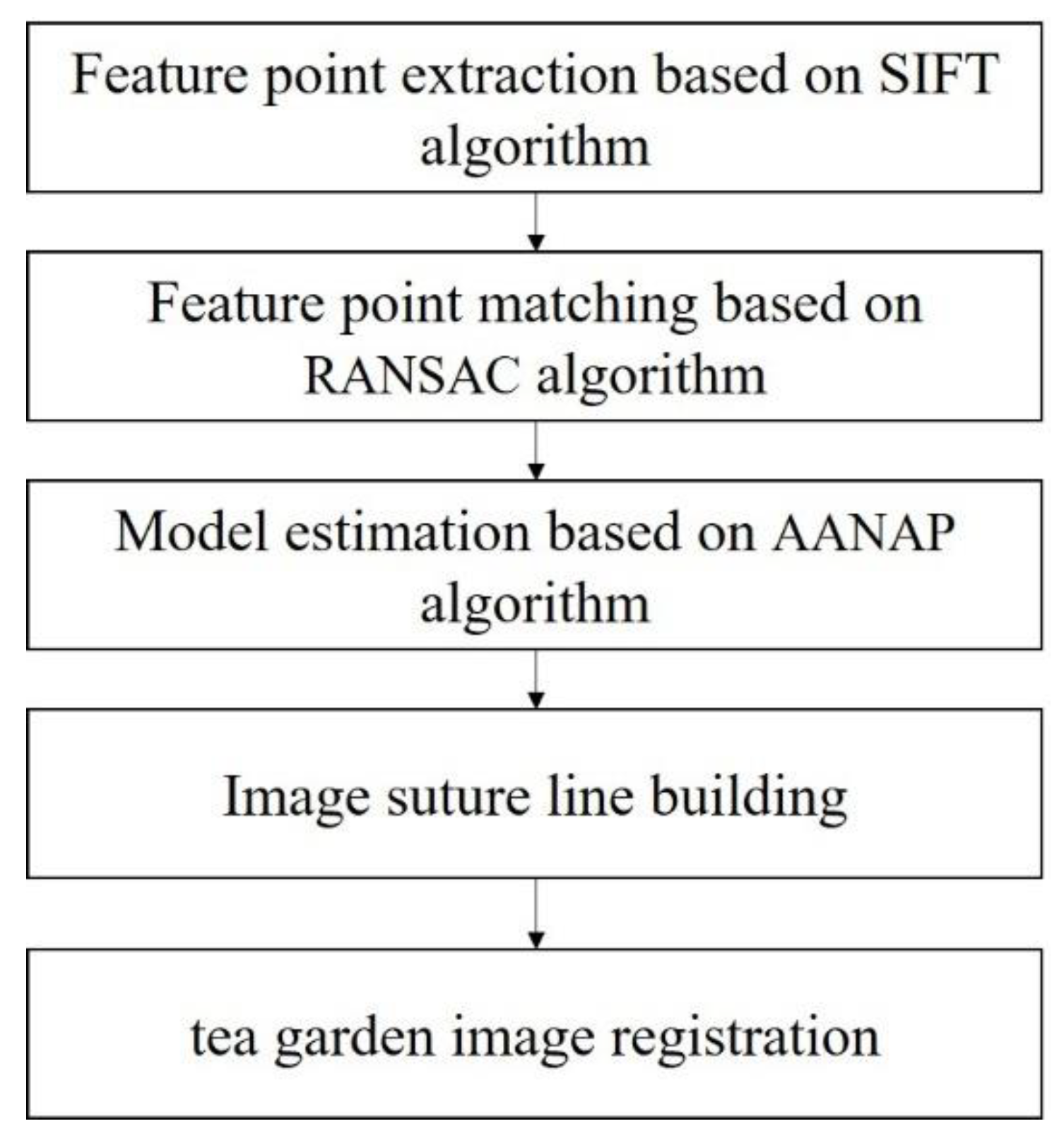
The flowchart of the image registration is shown in Figure 3.
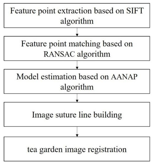
Figure 3.
Flowchart of the image registration.
2.4. Image Fusion Based on Improved Suture
The image suture line refers to the line of pixels that are most similar to each other in the overlapping area of the mosaic images. The two sides of the line are obtained from the content of two images, respectively. Then, the fusion strategy is carried out locally on both sides of the suture line. The suture strategy greatly reduces the overlap area, which in turn alleviates the problems of blurring and ghosting. The higher the quality of the suture found, the more natural the transition of the two images on both sides of the line will be.
In this paper, we adopted the optimal suture strategy based on the graph cutting method. Moreover, we improved the energy function to adapt to the tea garden image. This method ensures that the suture line is searched along the road as far as possible, which reduces the truncation and dislocation of the tea tree. By referring to the energy function based on the edge [27], the function is improved, as is shown in Formula (17):
where represents the final weight, represents the chromatic aberration term, represents the gradient difference, represents the texture difference term, and represents the penalty term.
For low-altitude tea garden images, due to the impact of different shooting angles and registration accuracy, tea trees on both sides of the suture line may not be aligned when stitching, resulting in truncation. In order to solve this problem, the improved suture method can position the dividing line as close to the strong edge of the image as possible, while searching the road in color, so that the dividing line is more difficult to detect and the stitching effect is more natural.
2.5. Tea Tree Extraction
2.5.1. Vegetation Index
By using vegetation indices, green plants in the images can be extracted. Not all the green plants need to be extracted; this is only necessary for tea trees.
In order to search for sutures along the road between the tea rows as far as possible, the image of the tea garden was observed, and it was found that there was a significant color difference between the road and the tea trees. The tea trees mainly presented a dark green color, while the road was mainly light yellow and red. Several vegetation indexes are compared in the Supplementary Materials (Supplementary Figures S1 and S2). Based on these results, the red–green ratio index (RGRI) was used in this paper to calculate the mask of tea trees.
where represent the
and
components in the RGB space, respectively. By using the ratio of pixels instead of each pixel, the image can represent the content of the green vegetation and other aspects; by setting a threshold range, we can obtain a good effect, as it can inhibit the images of hay, roads, and houses.
If we want to calculate and classify the neighborhood range of every pixel in the image, the workload for this exercise is undoubtedly great and unrealistic. In order to solve this problem, this paper obtains the points on the image at an average interval of a certain distance in both the horizontal and vertical directions, and then calculates the above features only for the neighborhood of these extracted points.
In the general images, there are many non-green features, such as roads, which can be directly eliminated by other vegetation indices after image preprocessing. The RGRI index, which has a better performance, was adopted to eliminate the content of non-green vegetation. Through the RGRI index of image processing, we set a threshold to retain most of the vegetation, with the likelihood of open operation, eliminating the legacy of the path points, and then expanding operations to tea trees in the middle of the hole to be filled, to obtain the final saturation mask image binarization. When extracting points in the image, the mask should be retained. Because the interference information extracted through the RGRI index mainly includes the target tea leaves and other trees and weeds with similar color characteristics, other contents that are directly removed are unnecessary and have no value of calculation, and the number of points can be further removed to reduce the calculation amount.
2.5.2. Image Features
In this paper, we extracted the color and texture features of tree images. By comparing several color models (HIS, LAB, and RGB), we observed that HSV had an intuitive expression of color tone, bright-colored degree, and degree of lights, which was convenient for color contrast. In its space, it is easier to track objects of a certain color, often used to divide objects of a specified color. The relationship between the RGB color model and HSV color model can be determined by the following Formula (19):
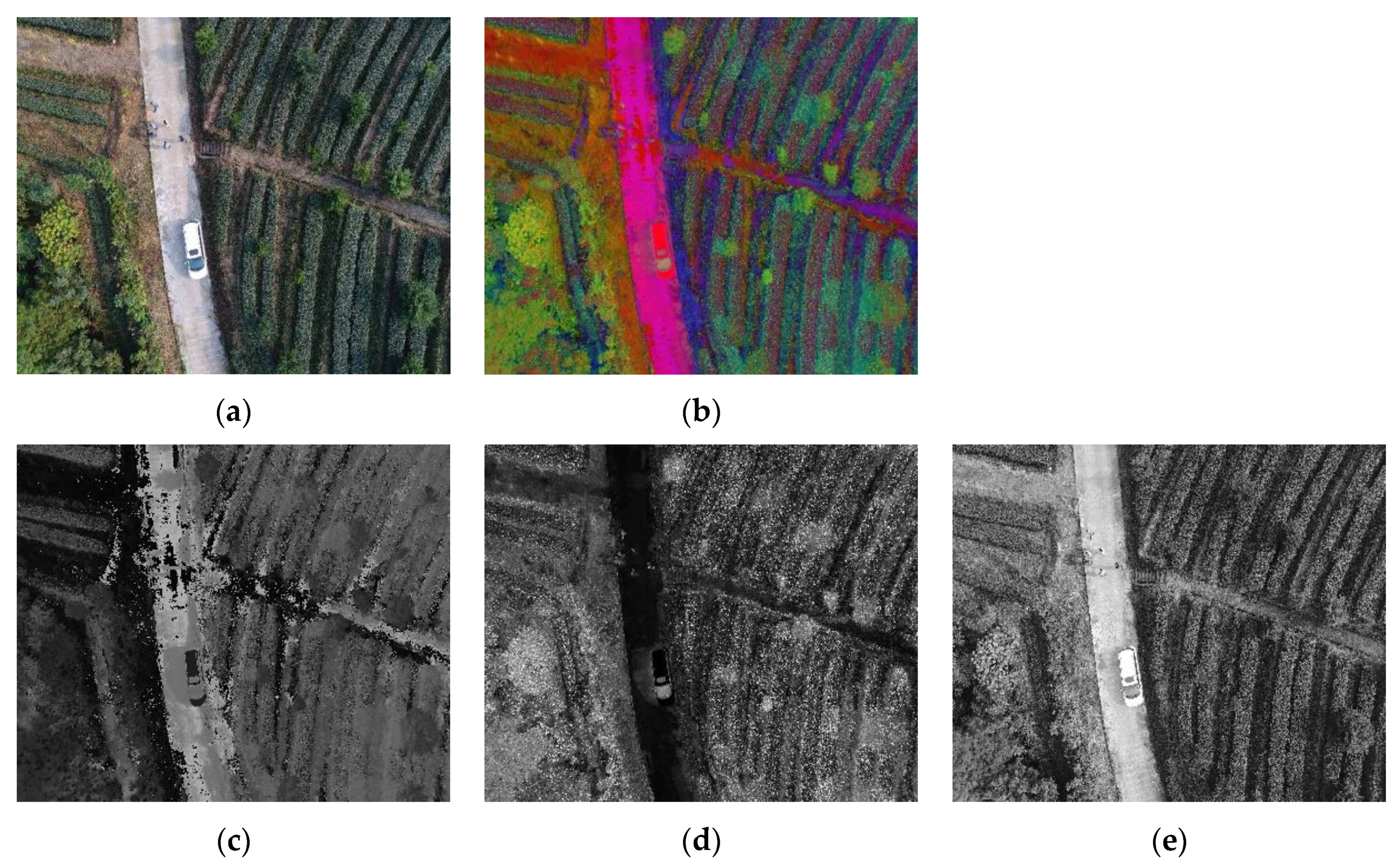
Figure 4 shows examples of the RGB model transferred to the HSV model and its H/S/V components.

Figure 4.
HSV model and components. (a) RGB model; (b) HSV model; (c) H component; (d) S component; and (e) V component.
2.5.3. Mean Shift Clustering
After the point set was extracted, as described in the previous section, the color and texture features were used for extraction. All the point sets obtained their own 18 characteristic values, and a range was set. When the difference between them was less than this range, the point was considered as belonging to the tea tree. However, concerning the method by which the threshold value is selected, the complexity and variability of each picture may lead to the fluctuation of the threshold value, resulting in the uncertainty of the final classification result. Moreover, if every point is calculated with the characteristic value of standard tea leaves, the number of calculations will be very large.
The image content mainly contains tea trees, trees, and other similar green vegetation. Therefore, each category has certain similarities between its point sets. According to this characteristic, we can first cluster the unclassified point sets, and then calculate an average value for each category of the clustering and compare it with the standard value. The comparison between the points is converted into the analysis between the classes, which greatly reduces the number of calculations. Because each image is different, the content of the information contained in the category is not consistent, so the clustering number set directly affects the subsequent clustering results; therefore, this paper adopted the adaptive mean shift clustering algorithm. This algorithm does not need to be artificially to set, but the algorithm itself is used to search the algorithm to determine the point gather class number.
Mean shift clustering is a mountain climbing algorithm, which seeks the region with the highest density in the data using the sliding the window technique and iterating a step-by-step method. The specific steps are as follows:
- (1)
- Randomly select a clustering point as the center, a sliding window with radius r, and calculate the highest point of data density in the current window as the new center.
- (2)
- Sliding the window to the new center and recalculating the cycle iteratively moves toward the direction of a higher density.
- (3)
- Convergence when there is no higher density in any direction.
- (4)
- The generated multiple clustering points are moved and converged in accordance with the above steps. When multiple centers converge and overlap, the points through which they pass are grouped into a class.
After clustering all the point sets by the means shift clustering algorithm, we need to analyze them to determine the target of the tea tree. The clustering situation and the standard eigenvalue of the tea tree are known, so we only need to use the standard value and the extracted point sets for comparative analysis. In order to avoid the influence of uneven characteristic values, we normalized the point sets and standard values and obtained their average values. Then, we calculated their Euclidean distance. The classes with minimum Euclidean distances were the markers for the tea tree.
2.5.4. Tea Tree Identification
In this paper, the k-nearest neighbor (KNN) algorithm was adopted, which is a simple and practical classical machine learning algorithm. The main idea was to compare a sample with a data set. The K data in the data set that are the most similar to the sample belong to that category, then, in that case, the sample belongs to that category.
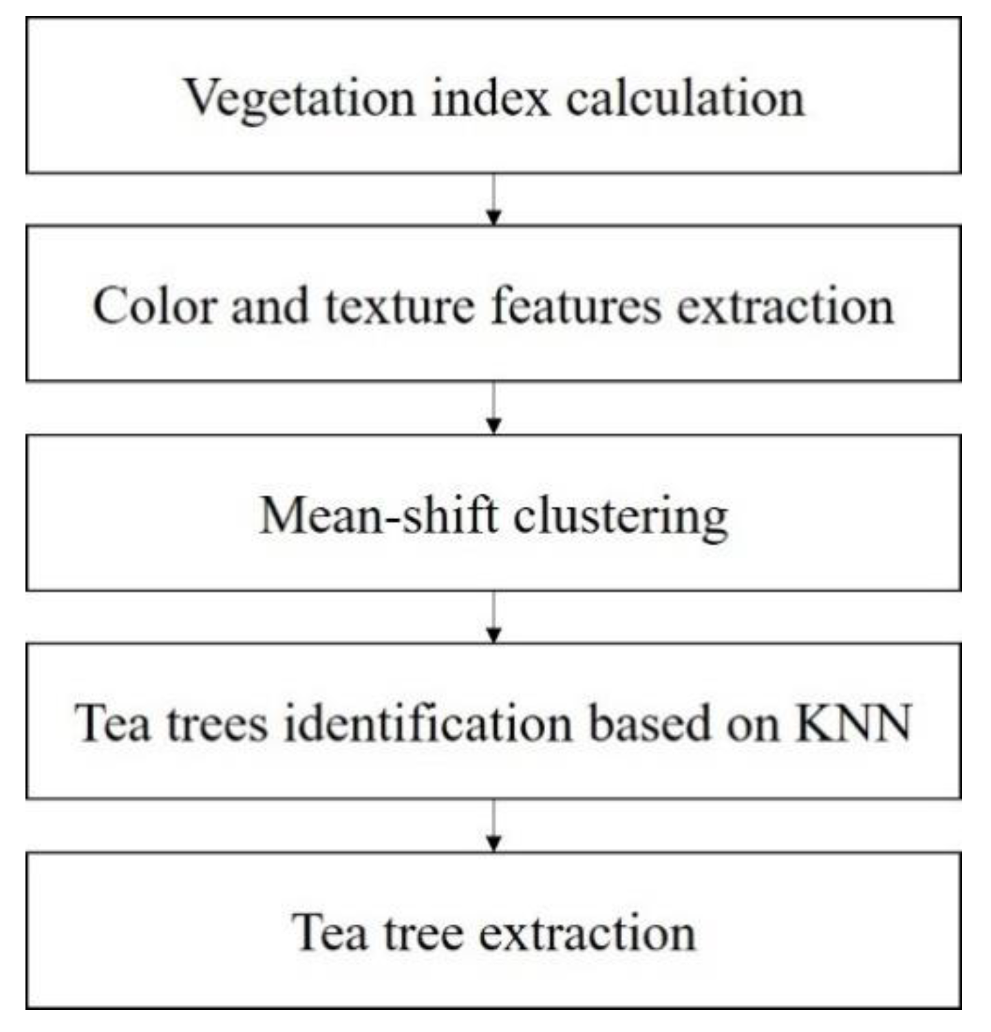
Through the KNN algorithm, the standard sample of tea leaves and the clustering point set are classified, and the standard sample is the most similar to the data of a certain class; this kind of point set is the target point set of the tea leaves for which we are searching. After the points are extracted separately, the scattered point sets are separated by a minimum outer polygon and a certain degree of morphological operation to remove miscellaneous points and expand the boundary. Finally, the tea tree targets distributed in multiple places are fitted. In the fitting stage, if the number of each independently connected point set is less than a certain number, it is immediately removed. For most of the cases, there are isolated clusters of very similar green vegetation. Figure 5 present the flowchart of the tea tree extraction.
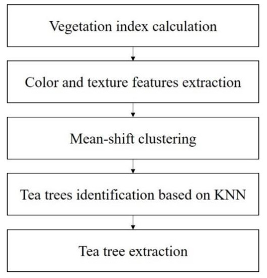
Figure 5.
Flowchart of tea tree extraction.
2.6. Results Evaluation
There are two aspects to evaluate the results of the study: visual comparison and 4 evaluation rates.
First, we used AutoStitch, a commercial software to evaluate the image mosaic results. We used the software and our method to stitch the same images. In traditional methods [28,29], if the edge between the images is not visible to human eyes, the mosaic image is regarded as “applicable”. Some of the literature states that if the result image is complete, clear, or there is no obvious distortion, the stitching algorithm is appropriate and practical [30]. Therefore, our method resulted in “no visible edges” in the manner of commercial software, or if the visual results are better, the mosaic image is regarded as “good”.
Then, we calculated the rates to evaluate the tea tree extraction results. The tea trees are shown in the images as pixels; therefore, we counted the pixels. The ground truth pixels were apprehended by the human eye by using Photoshop software, including tea tree pixels from both the raw images and mosaic images. The four rates used were the accuracy rate, error rate, omission rate and the union of the intersection ratio (IOU) calculated as Formulas (20)–(23):
3. Results and Discussion
3.1. Tea Garden Image Registration
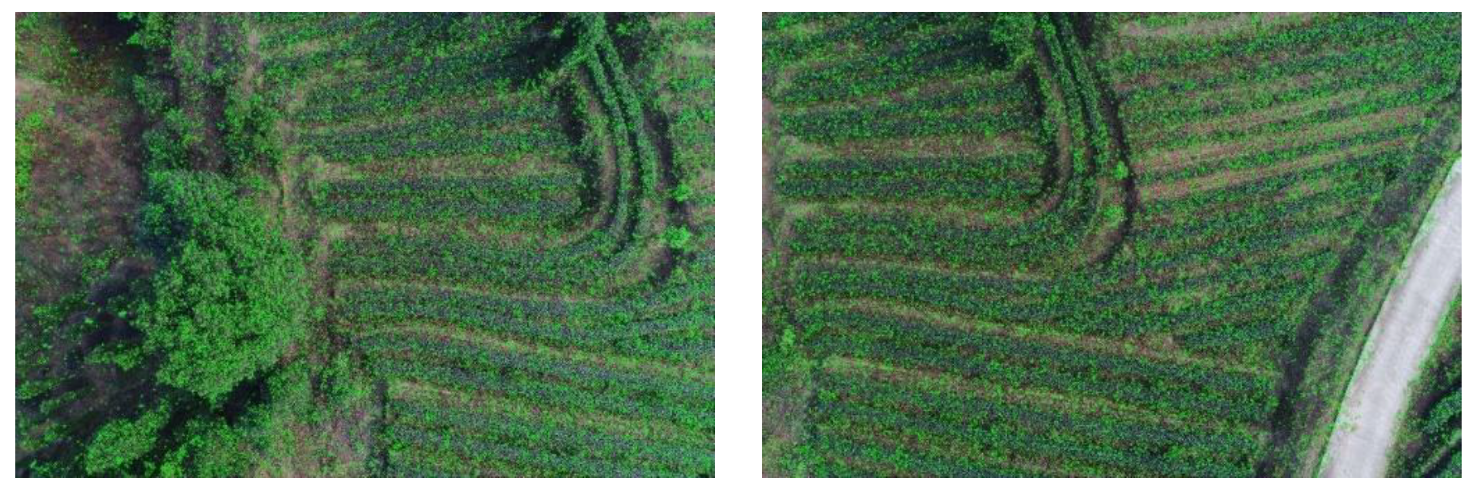
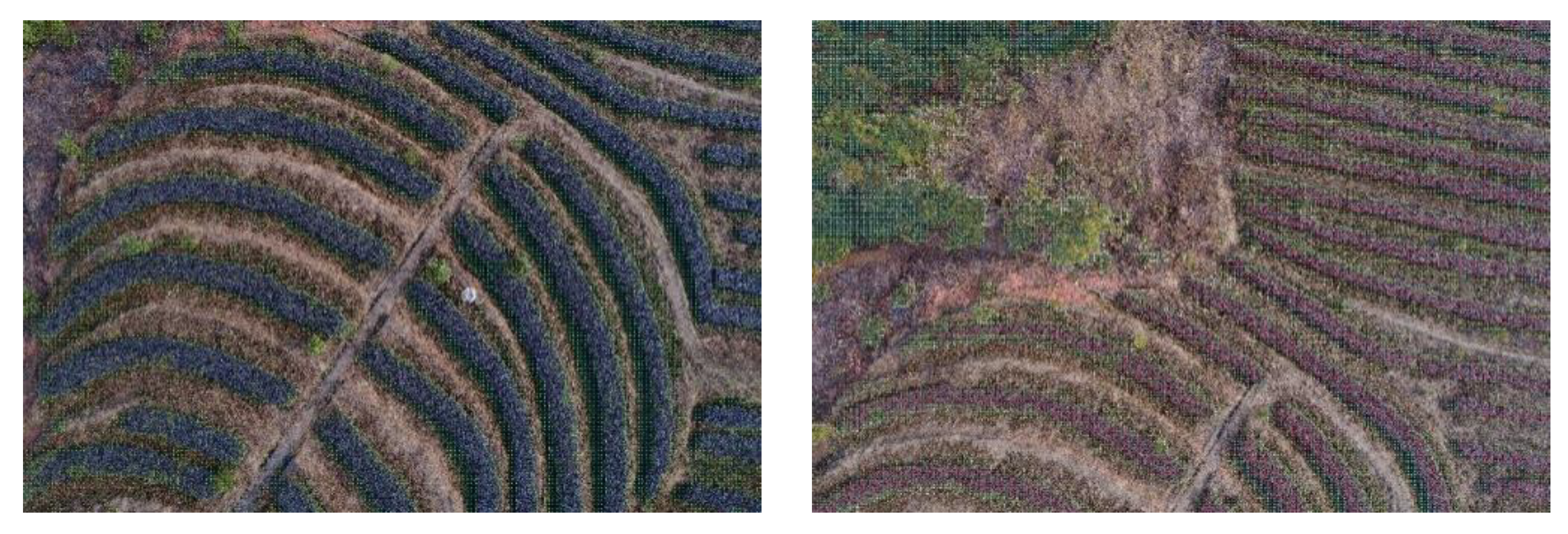
The feature points extraction effect of the SIFT algorithm is shown in Figure 6; the green points represent the extracted ones.
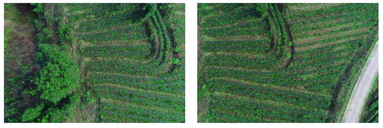
Figure 6.
SIFT feature points in the tea garden images.
In theory, the closer the distance of the two feature points, the higher the matching rate, which shows that they are more similar [27]. However, according to Figure 6, the actual situation is not entirely the same as the theory. The most similar matching points should appear in the overlapping areas, but they, in fact, do not match. Moreover, a feature point is close to two or even more points simultaneously. If the closest point is simply chosen as the matching point, it is not necessarily correct, which may lead to mismatching.
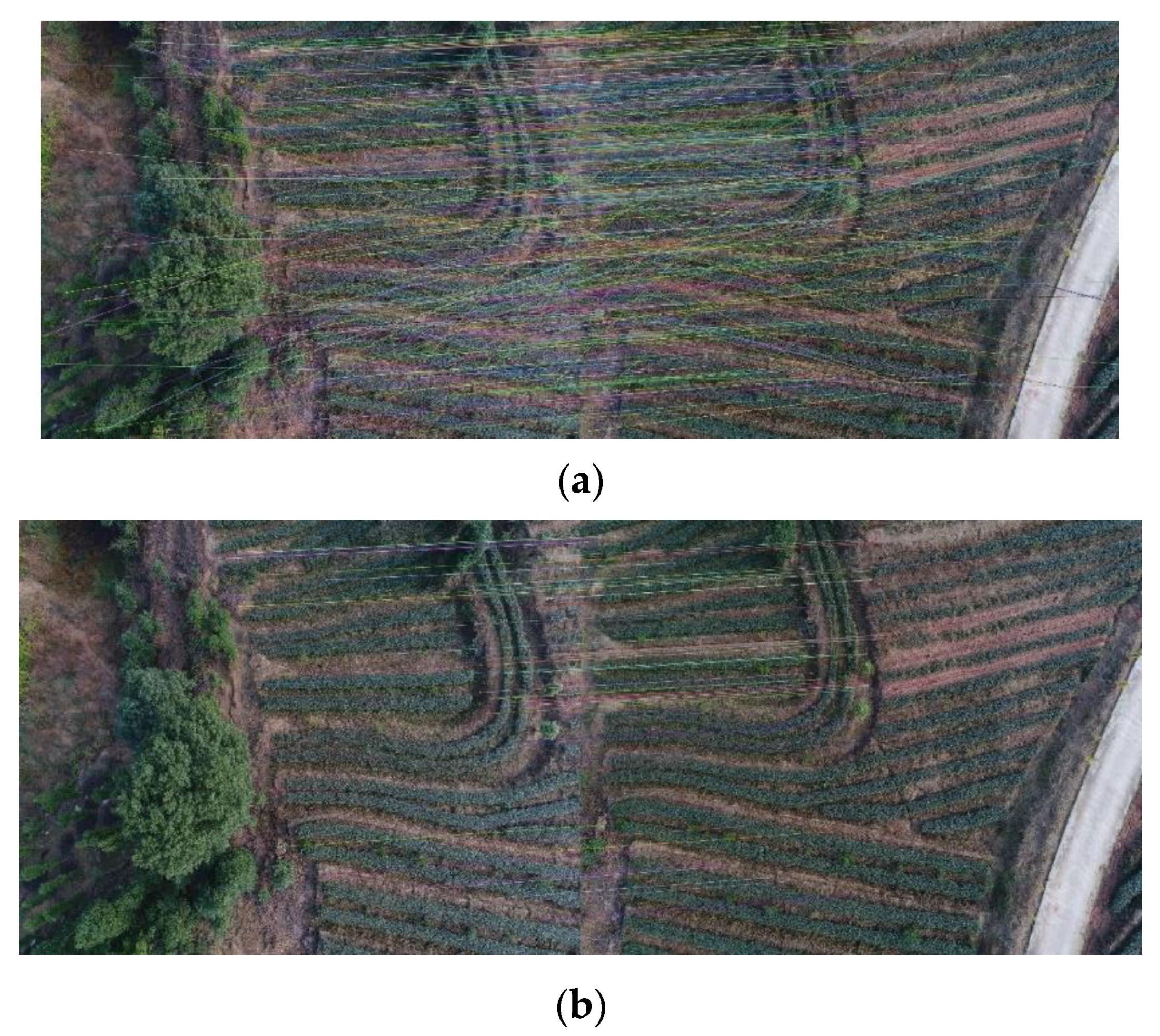
In order to reduce the number of false matchings, we need rough matching to determine the feature point pairs initially, and then remove the false matching point pairs through fine matching. The matching effect of feature points is presented in Figure 7.
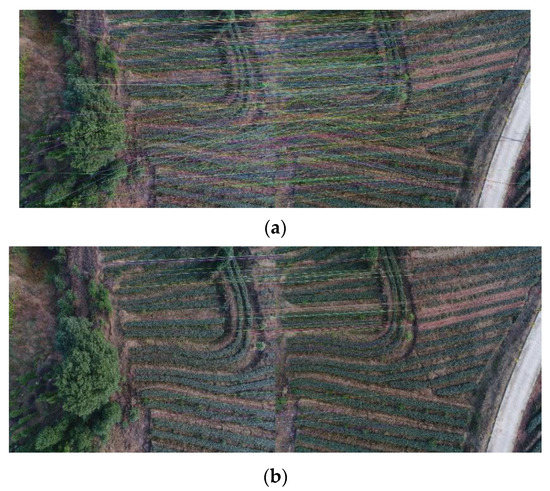
Figure 7.
Matching effects of the (a) rough match and (b) exact match.
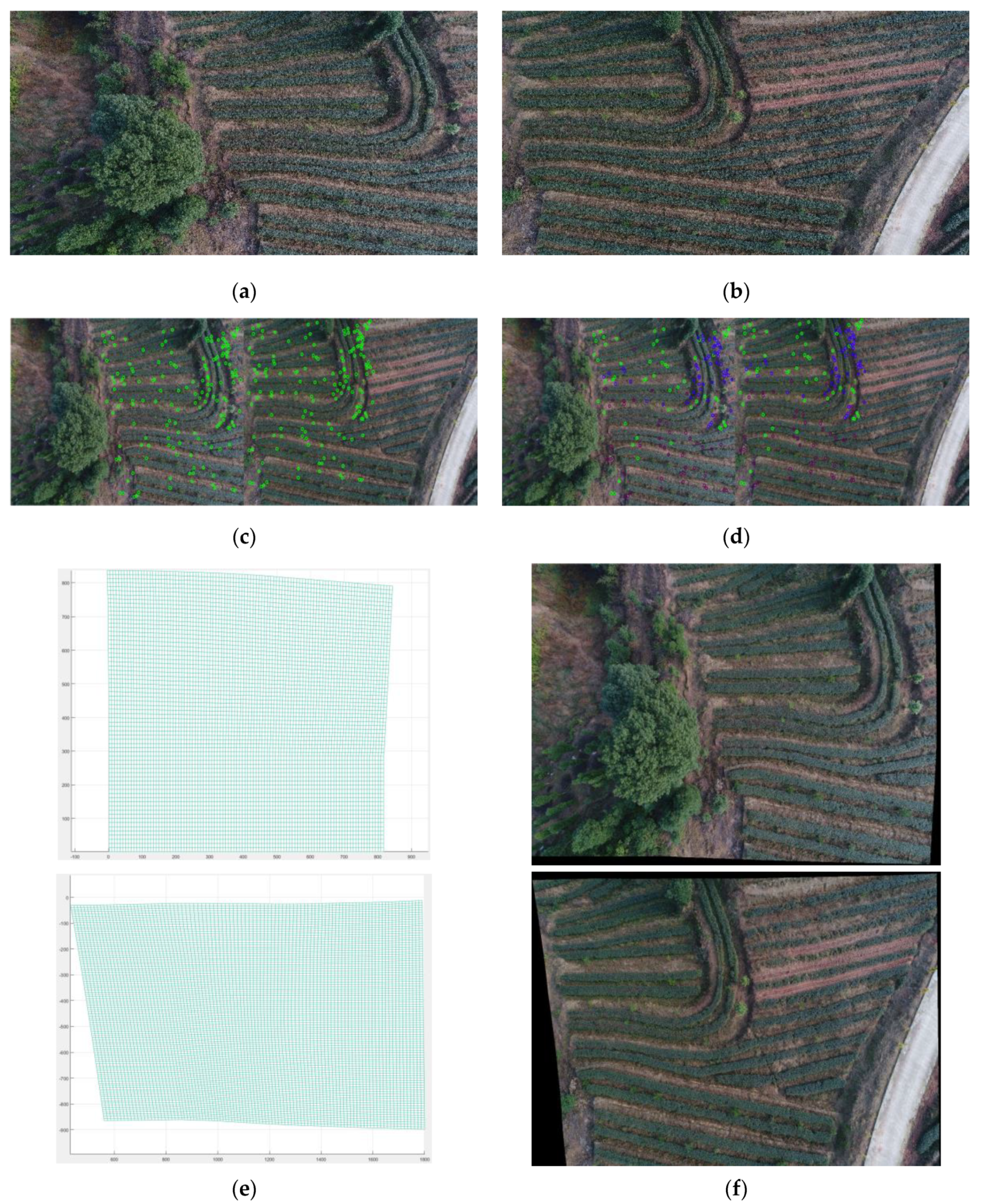
The process of grid partitioning and alignment are shown in Figure 8. SIFT was used to extract the feature point pairs retained after the fine matching of the feature points, and then different thresholds were set through RANSAC to obtain the global similarity transformation matrix with the minimum included angle. The MDLT efficient algorithm provided by the author was used to obtain the homograph matrix in the grid. Then, after integrating each grid, the final local single sex matrix and transformation are calculated, as shown in Figure 8e. In 2013, Zargoza and Chin et al. proposed an APAP algorithm based on grid partitioning [31]. By evenly dividing the image into multiple grid regions, each grid would calculate its own transformation matrix, which greatly improved the degree of image alignment. For the deformation problem in the non-overlapping area, the adaptive AANAP algorithm [28] proposed by Lin C et al. was improved, based on the APAP algorithm, by adding a linearized projection transformation, automatically estimating the global similarity transformation in the overlapping area, and making corresponding adjustments to the target image. At the same time, a variety of improved algorithms used to add constraints [32] were proposed successively, such as adding line-keeping constraints based on the APAP algorithm to reduce distortion [33]. In our study, the reference image and target image were overlayed. Through the mesh deformation (Figure 8e), for most of the area, the fuzzy linear and ghosting were slowed down. By using the linear fusion, the original border splicing trace can be observed clearly.
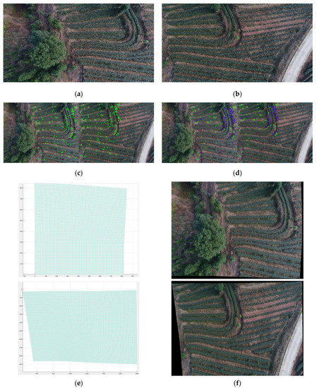
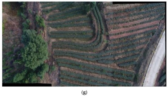
Figure 8.
Tea garden image registration by the AANAP algorithm. (a) Reference image; (b) target image; (c) image with extracted feature points by the SIFT algorithm; (d) image with selected feature points; (e) mesh division and deformation; (f) image transformation result; and (g) results by the AANAP algorithm.
3.2. Tea Garden Image Fusion
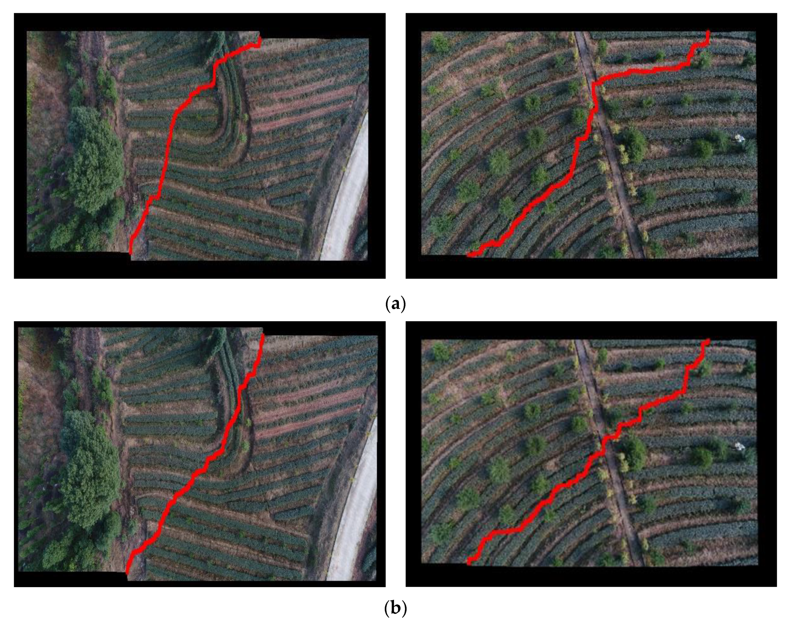
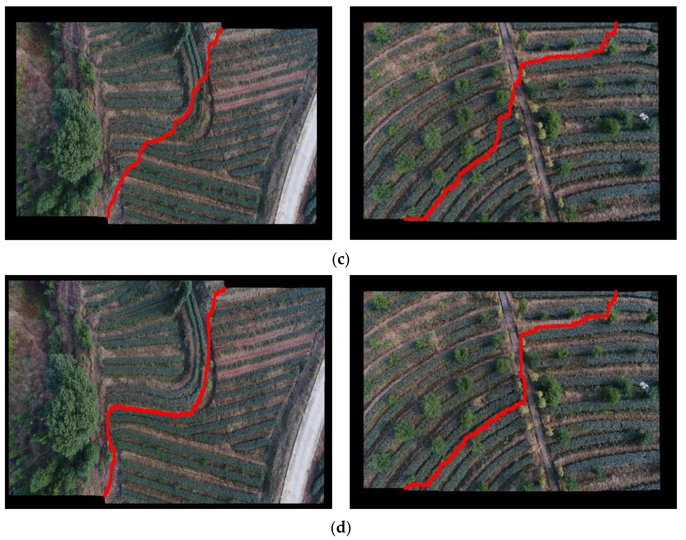
In this paper, the results of the “color” feature energy function, “gradient” feature, “color + gradient” and energy function proposed are shown in Figure 9. The red lines are the searched suture lines by different features.
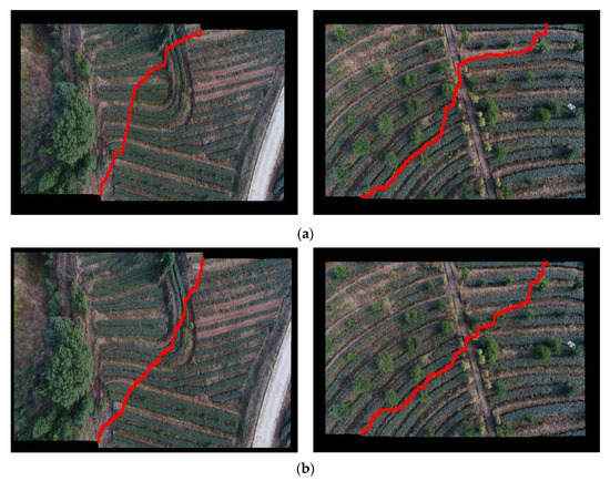
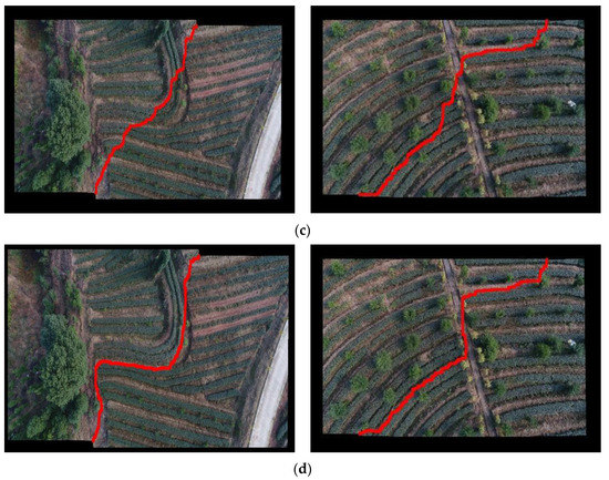
Figure 9.
Results of the suture lines with different energy functions (a) based on the “color” feature, (b) “gradient” feature, and (c) “color + gradient” feature (d) in this study.
As shown in the above figures, the bold, red, solid lines are used to display the sutures searched. The image suture line refers to the line of pixels that are most similar to each other in the overlapping area of mosaic images. The two sides of the line are taken from the content of two images, respectively. The suture strategy greatly reduces the overlap area, which in turn alleviates the problems of blurring and ghosting. The higher the quality of the obtained suture, the more natural the transition of the two images on both sides of the line. Most sutures searched based on the color, texture, or traditional energy function [34,35] combine color and texture and cross the walking spaces of the tea tree area. They increased the probability of misplaced truncation. The algorithm used in this study first searches along the road between the tea trees, reducing the number of tea trees passing through, ensuring the continuity and integrity of the tea trees as much as possible, which conforms to human visual perception and facilitates subsequent agricultural analysis.
In this paper, we also represented other algorithms for analysis, as shown in Figure 10.

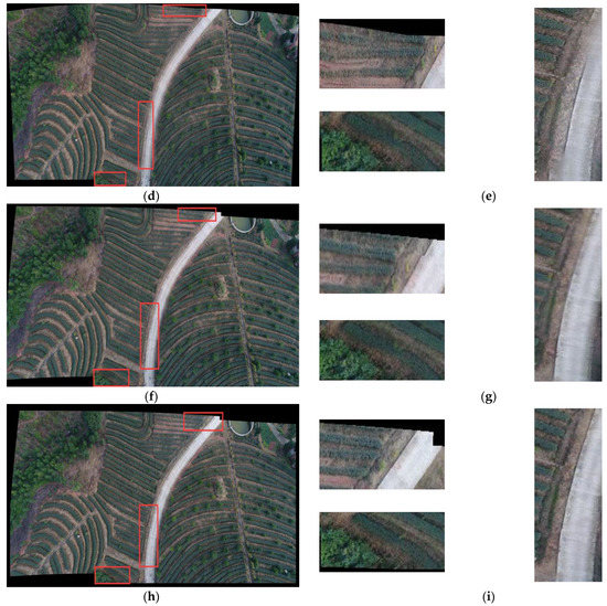
Figure 10.
Results of AutoStitch, AANAP and the algorithms used in this study. (a) Reference images; (b) target image; (c) suture line results of (a,b) in this study; (d) results in AutoStitch; (e) magnified images in red frames of (d); (f) results in AANAP; (g) magnified images in red frames of (f); (h) results in this study; and (i) magnified images in red frames of (h).
It can be observed in Figure 10 that if the overlapping area is small, there are errors in stitching traces at the boundary. The errors are not obvious in images of an original size (Figure 10d,f), which do not affect the application of the image. In this way, the stitching results of the AutoStitch software and AANAP algorithm have good effects. When the images were magnified, the results are different. When AutoStitch searches for the suture lines, there is a dislocation in the road, shown in Figure 10e, while the AANAP algorithm performs linear fusion on the whole overlapping area, so the image becomes fuzzy and some tea tree details are lost (Figure 10g). The algorithm in this paper solved the boundary stitching traces (Figure 10i), and achieved good stitching results by the best suture line along the boundary and by crossing the tea tree as little as possible, which verified the effectiveness of the algorithm in this paper.
3.3. Tea Tree Extraction
3.3.1. Vegetation Index
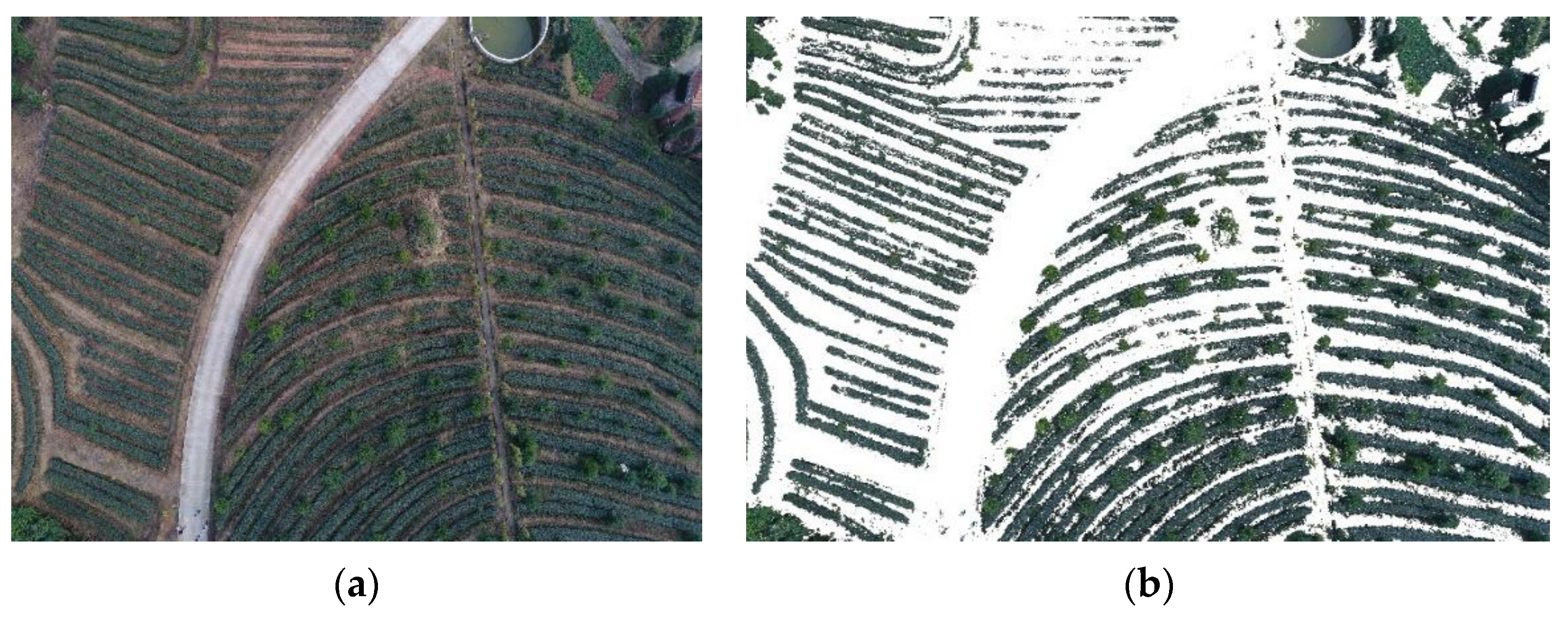
By replacing the pixel value of each pixel with the ratio, the image obtained can better distinguish green vegetation from other contents. By setting a threshold range, a good effect can be achieved, and most of the other withered grass, roads and houses can be better suppressed. The overall effect is shown in Figure 11.

Figure 11.
Original image (a) and the image with RGRI features (b).
In Figure 11b, the road and the walking spaces between the tea trees are inhibited, while the green features of the tea garden, including the green trees, pools, and other green crops, are retained. Most non-green features, such as the roads, can be directly eliminated by the RGRI index calculation with a set threshold. Then, an open operation was used to eliminate the legacy of the path points, and expanding operations were used to fill the hole of tea tree (r = 5). Finally, we obtained the binary mask image (Figure 12c). If the extracted point is in the image, it is retained; otherwise, is deleted. By using this method, we can reduce the calculation. The steps are shown in Figure 12.
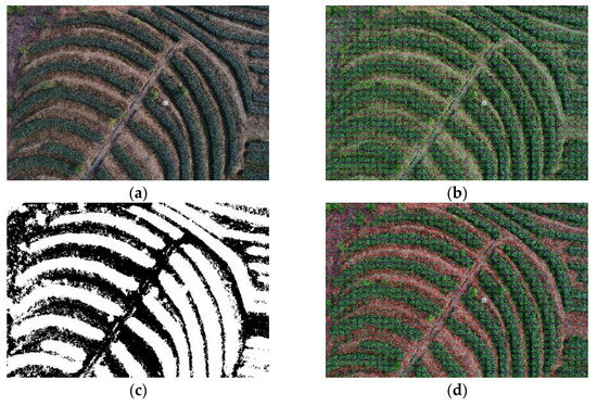
Figure 12.
Point set extraction and filtering. (a) Raw image; (b) image by point set extraction; (c) binary mask image calculated by RGRI indices; and (d) image after filtering.
As shown in the figures above, the size of the image is 5472 × 3648, with a total of 19,961,856 pixels. If every pixel of the image is calculated, the workload is large and impractical for application. Therefore, we applied points to the image at a certain distance between the horizontal and vertical directions. Assuming that the spacing is 20 pixels, 273 and 182 points can be selected in the horizontal direction and the vertical direction, respectively, with a total of 49,686 points, about two thousandths of the original picture, and then filtered by the binary template of RGRI. There are only 29,274 points remaining, and as the spacing is increased, the computation shrinks even further.
3.3.2. Tea Tree Identification
By mean shift clustering, the tea trees and other green plants were categorized as different point sets. According to their features, we can cluster the unclassified point sets. We calculated the mean value of each point set. Then, we compared them with the standard value. By using this method, we do not need to compare points by points, which greatly reduces the number of calculations. The results are shown in Figure 13.
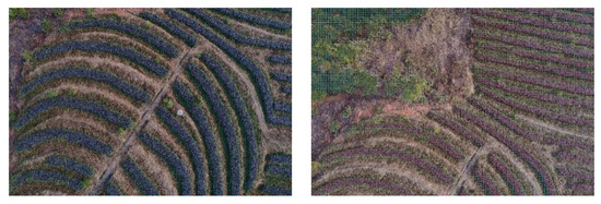
Figure 13.
Mean shift clustering results of different image examples.
Because each image obtains different clustering results and numbers of clusters, the colors are randomly generated, leading to the tea trees in different images being displayed in different colors. For example, in Figure 13, the clustering results of the left and right images are 16 and 22 categories, respectively. Most tea trees are grouped into one category, while the other green plants are displayed and distinguished by different color point sets. However, this method is not suitable for images with a complex content and large amounts of information.
The tea group and clustering point sets are classified by the KNN algorithm (n = 20). KNN classification and tea tree extraction is shown in Figure 14. If one clustering point set is close to the standard sample, it is the target one. the point set is marked green (Figure 14b). Then, smallest peripheral polygons are carried out for the scattered point of morphological operations (r = 5). By using this method, the miscellaneous points are removed and the boundaries are expanded (Figure 14c). Finally, the tea tree targets distributed in multiple places are fitted. If the number of one point set is less than 20, it is removed from the extraction results.
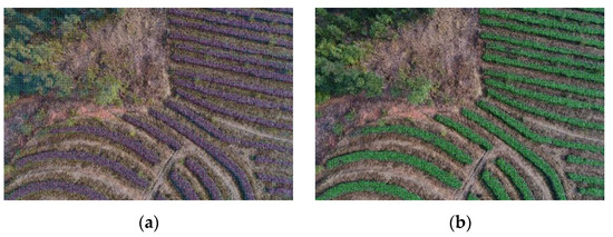
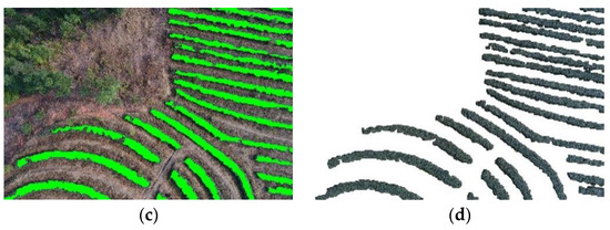
Figure 14.
KNN classification and tea tree extraction. (a) Mean shift clustering results; (b) KNN classification results; (c) contour fitting result; and (d) extraction results.
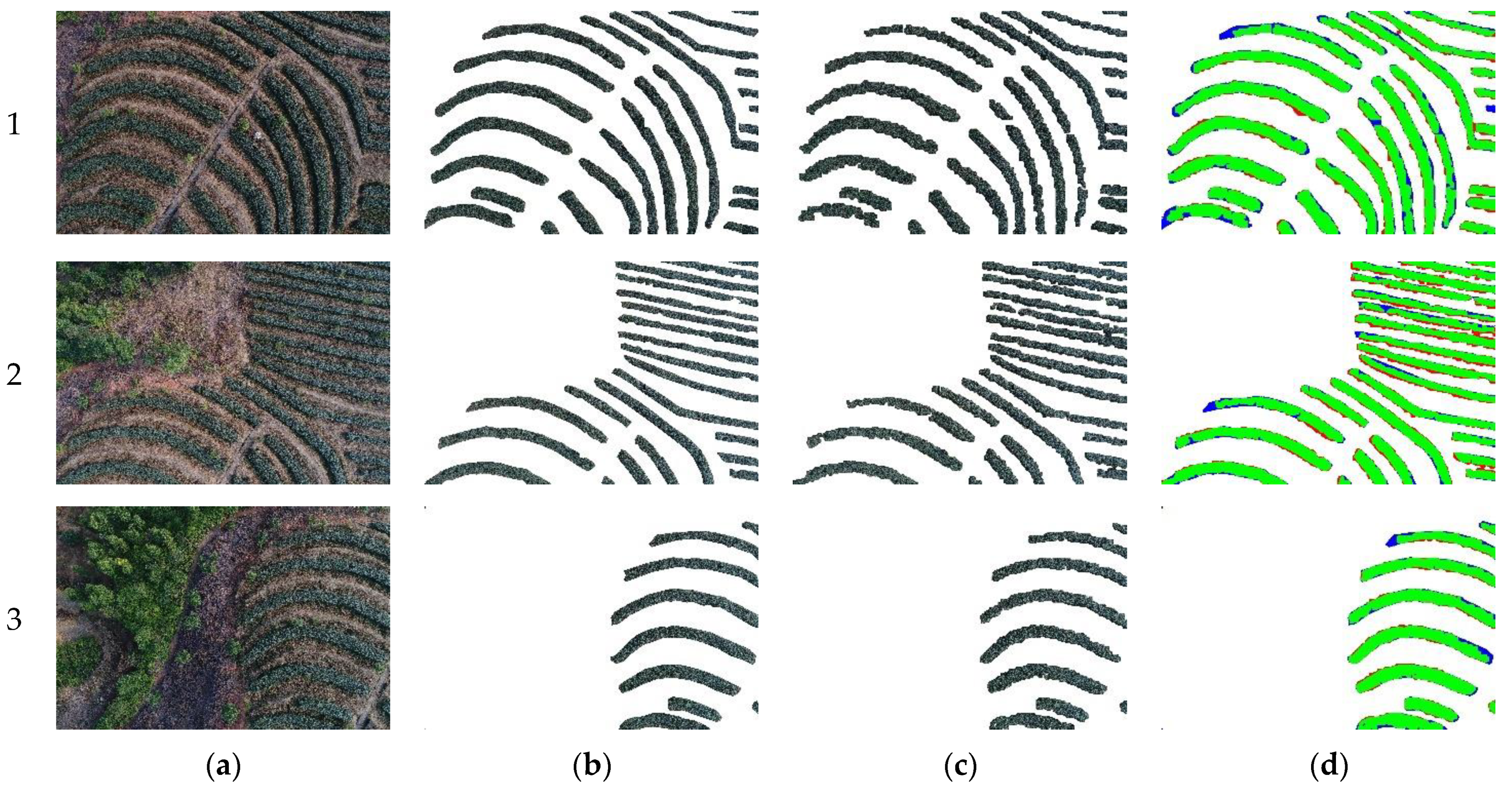
After extracting the tea trees from the images, we utilized Photoshop software to artificially extract the tea tree pixels from the tea garden image as the ground truth. The comparison between the ground truth and method performed in this study are shown in Figure 15. The green pixels represent the correctly extracted part when the extracted pixels matched the ground truth; the red pixels represent the incorrectly extracted part when the extracted pixels did not match the ground truth; and the blue pixels represent the missed extracted part of the tea tree.

Figure 15.
Comparison images of the ground truth and method in this study. (a) Raw image; (b) tea tree extracted by humans; (c) tea tree extracted in this study; and (d) result of the contrast between (b,c).
It can be observed in Figure 15c,d that the algorithm in this study eliminated the interference information of the roads, trees, weeds, and tea tree boundary well, and effectively extracted the tea tree target. However, the result was sensitive to light, which especially caused occlusion. Some clustering of the tea tree points was classified into another kind of point set. Additionally, as the complexity of the scene increased, some trees remained as tea trees.
Figure 15 presents the comparison images of single images. Figure 16 presents the results of the application of the algorithm to the tea garden mosaic images.
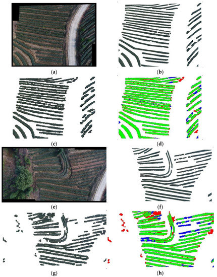
Figure 16.
Contrastive example of the tea tree extraction from the tea garden mosaic images. (a) mosaic image 1; (b) tea tree extracted as the ground truth of (a); (c) tea tree extracted in this study; (d) result of the contrast between (b) and (c); (e) mosaic image 2; (f) tea tree extracted as the ground truth of (e); (g) tea tree extracted in this study of (e); and (h) the result of the contrast between (f,g).
It can be observed in Figure 16 that the error or omission occurs on the tea tree border (the blue blocks in Figure 16d), if the scenario is simple, similar to Figure 16a. However, in more complex scenarios, including other plants (Figure 16e), most of the trees and weeds were removed, but some were still reserved (the red blocks in Figure 16h), especially in the sparse areas and the shadows (Figure 16g). As the mosaic image contains more interference information, the result decreases.
We analyzed the pixels in all the images, including the tea tree pixels extracted in this study, the ground truth pixels, and the missed extracted tea tree pixels to calculate the 4 rates. These are the accuracy rate, error rate, omission rate and IOU. In this paper, the accuracy and error rates are based on the proportion of the pixel area of the extracted tea trees. The omission rate is based on the proportion of the area of the tea trees extracted manually, and the IOU of manual extraction and extraction in this paper. The results of the three image groups and their mosaic images are shown in Table 1. During the calculation, the following data were used: the size of the raw image was 5472 × 3648, with a total of 19,961,856 pixels; the spacing of the clustering was set to 20 pixels; 273 and 182 points of each raw image were selected in the horizontal and vertical directions, respectively, with a total of 49,686 points, about two thousandths of the original picture, and then filtered by the binary template of RGRI. In this way, there are only 29,274 points of each image remaining; the threshold value of RGRI is 0 to 0.9; the r of the scattered point for morphological operations is set to 5; and the KNN algorithm, n of neighbors is set to 20.

Table 1.
Results of this method in the image mosaic and tea tree extraction.
According to the content presented in the table above, the algorithm in this paper can accurately extract more than 84% of the tea trees. With the decrease in the height of the image, the details of the tea trees increased alongside the interference information, the accuracy rate decreased from 93.28% to 84.91%, and the error rate increased from 6.72% to 15.09%. The omission rate and IOU also decreased, especially in the mosaic image (Mosaic 1 and Mosaic 2). The tea tree extraction accuracy rates in the mosaic images are 84.96% at 30 m high, and 79.94% t 60 m high. With the increase in the image content from 100 m high to 30 m high, the IOU of the mosaic images decreased in the single images. While the IOU in the mosaic images increased from 67.19% to 77.17%, the flight height decreased from 60 m to 30 m. This represents the advantage of our method.
The images collected in this paper are all visible light waves, which have limitations in the extraction of tea trees. The algorithm may be sensitive to light and sparsely situated tea trees. If the selection of the feature vectors is not reliable, which is not robust to illumination, it causes a situation in which the extracted standard tea tree features cannot meet the overly complex environment. The feature vectors constructed by color and texture are still deficient in distinguishing the complex content. This boundary problem is not considered in the calculation of the feature vectors, and the instability of the tea tree boundary can be clearly observed in the results. In the actual test, the color features were found to have a greater impact.
4. Conclusions
In the present study, we used a drone to take RGB images of a tea garden from three different heights. Then, we improved the energy function to realize the image mosaicking of the tea garden. The suture line searched using this method ensured the continuity and integrity of the tea trees as much as possible. After image mosaicking, we built a feature vector to extract the tea trees from the tea garden images. By comparing our method with the ground truth, the algorithm in this paper effectively distinguishes and eliminates most of the interference information from the images. The IOU in a single mosaic image was more than 80%, and the omission rate was 10%. The extraction results in accuracy ranging from 84.91% to 93.82% for the different height levels (30 m, 60 m and 100 m) of the single images. The tea tree extraction accuracy rates in the mosaic images are 84.96% at a height of 30 m and 79.94% at a height of 60 m. Facing the complicated and changeable environment, similar to the tea gardens, this paper proposes a strategy to distinguish the tea trees from the information concerning similar green vegetation. How to reduce the degree of deformation or dislocation truncation in tea garden image mosaicking is an important and difficult research area. Our future work aims to collect more information and facilitate the subsequent agricultural analysis, multispectral and hyperspectral.
Supplementary Materials
The following supporting information can be downloaded at: https://www.mdpi.com/article/10.3390/agriengineering4010017/s1, Figure S1. extraction examples by vegetation indexes; Figure S2 RGRI index extraction effect of different thresholds. References [36,37] are cited in the Supplementary Materials.
Author Contributions
Conceptualization, J.L. and Z.G.; methodology, Y.X.; software, Y.X.; validation, Y.X., J.L. and Z.G.; formal analysis, J.L.; writing—original draft preparation, J.L.; writing—review and editing, J.L. All authors have read and agreed to the published version of the manuscript.
Funding
This research was funded by the Sichuan Science and Technology Program grant number 2021YEN0020.
Institutional Review Board Statement
Not applicable.
Informed Consent Statement
Not applicable.
Data Availability Statement
Not applicable.
Acknowledgments
The authors thank Wang Wei from the Yibin Agricultural Machinery Institute for his support during the experiment in Yibin.
Conflicts of Interest
The authors declare no conflict of interest.
References
- Li, X.; Feng, R.; Guan, X.; Shen, H.; Zhang, L. Remote Sensing Image Mosaicking: Achievements and Challenges. IEEE Geosci. Remote Sens. Mag. 2019, 7, 8–22. [Google Scholar] [CrossRef]
- Zhang, H.; Wang, L.; Tian, T.; Yin, J. A Review of Unmanned Aerial Vehicle Low-Altitude Remote Sensing (UAV-LARS) Use in Agricultural Monitoring in China. Remote Sens. 2021, 13, 1221. [Google Scholar] [CrossRef]
- Murugan, D.; Garg, A.; Singh, D. Development of an Adaptive Approach for Precision Agriculture Monitoring with Drone and Satellite Data. IEEE J. Sel. Top. Appl. Earth Obs. Remote Sens. 2017, 10, 5322–5328. [Google Scholar] [CrossRef]
- Pandey, A.; Pati, U.C. Image mosaicing: A deeper insight. Image Vis. Comput. 2019, 89, 236–257. [Google Scholar] [CrossRef]
- Xie, R.; Tu, J.; Yao, J.; Xia, M.; Li, S. A robust projection plane selection strategy for UAV image stitching. Int. J. Remote Sens. 2019, 40, 3118–3138. [Google Scholar] [CrossRef]
- Wang, Z.; Yang, Z. Review on image-stitching techniques. Multimedia Syst. 2020, 26, 413–430. [Google Scholar] [CrossRef]
- Keller, Y.; Averbuch, A.; Israeli, M. Pseudo-Polar Based Estimation of Large Translations Rotations and Scalings in Images. IEEE Trans. Image Processing 2005, 2, 201–206. [Google Scholar] [CrossRef]
- Kuglin, C.D.; Hines, D.A. The phase correlation image alignment method. IEEE Int. Conf. Cybern. Soc. 1975, 163–165. [Google Scholar]
- De Castro, E.; Morandi, C. Registration of Translated and Rotated Images Using Finite Fourier Transforms. IEEE Trans. Pattern Anal. Mach. Intell. 1987, 9, 700–703. [Google Scholar] [CrossRef]
- Yang, L.; Jw, A.; Ky, A. Modified phase correlation algorithm for image registration based on pyramid. Alex. Eng. J. 2022, 61, 709–718. [Google Scholar]
- Zitová, B.; Flusser, J. Image registration methods: A survey. Image Vis. Comput. 2003, 21, 977–1000. [Google Scholar] [CrossRef] [Green Version]
- Zhang, L.; Wang, L.; Yang, B.; Niu, S.; Han, Y.; Oh, S.K. Rapid Construction of 4D High-Quality Microstructural Image for Cement Hydration Using Partial Information Registration. Pattern Recognit. 2022, 124, 108471. [Google Scholar] [CrossRef]
- Copik, M.; Grosser, T.; Hoefler, T.; Bientinesi, P.; Berkels, B. Work-Stealing Prefix Scan: Addressing Load Imbalance in Large-Scale Image Registration. IEEE Trans. Parallel Distrib. Syst. 2021, 33, 523–535. [Google Scholar] [CrossRef]
- Jing, R.; Deng, L.; Zhao, W.J.; Gong, Z.N. Object-oriented aquatic vegetation extracting approach based on visible vegetation indices. J. Appl. Ecol. 2016, 27, 1427–1436. [Google Scholar]
- Gitelson, A.A.; Viña, A.; Ciganda, V.; Rundquist, D.C.; Arkebauer, T.J. Remote estimation of canopy chlorophyll content in crops. Geophys. Res. Lett. 2005, 32, L08403. [Google Scholar] [CrossRef] [Green Version]
- Ciganda, V.S.; Gitelson, A.A.; Schepers, J. How deep does a remote sensor sense? Expression of chlorophyll content in a maize canopy. Remote Sens. Environ. 2012, 126, 240–247. [Google Scholar] [CrossRef]
- Torres-Sánchez, J.; Peña, J.M.; de Castro, A.I.; López-Granados, F. Multi-temporal mapping of the vegetation fraction in early-season wheat fields using images from UAV. Comput. Electron. Agric. 2014, 103, 104–113. [Google Scholar] [CrossRef]
- Meyer, G.E.; Neto, J.C. Verification of color vegetation indices for automated crop imaging applications. Comput. Electron. Agric. 2008, 63, 282–293. [Google Scholar] [CrossRef]
- Torres-Sánchez, J.; Lopez-Granados, F.; De Castro, A.I.; Peña-Barragan, J.M. Configuration and Specifications of an Unmanned Aerial Vehicle (UAV) for Early Site Specific Weed Management. PLoS ONE 2013, 8, e58210. [Google Scholar] [CrossRef] [Green Version]
- Rasmussen, J.; Nielsen, J.; Garciaruiz, F.; Christensen, S.; Streibig, J.C. Potential uses of small unmanned aircraft systems (UAS) in weed research. Weed Res. 2013, 53, 242–248. [Google Scholar] [CrossRef]
- An, L.; Guo, B.-L.; He, W.-P.; Hou, J. A Method of Point Cloud Classification Using Multi-scale Dimensionality Features and Transductive Learning. DEStech Transactions on Computer Science and Engineering. In Proceedings of the 2018 International Conference on Computational Modeling, Simulation and Mathematical Statistics (CMSMS2018), Xi’an, China, 24–25 June 2018. [Google Scholar]
- Huang, H.; Brenner, C.; Sester, M. A generative statistical approach to automatic 3D building roof reconstruction from laser scanning data. ISPRS J. Photogramm. Remote Sens. 2013, 79, 29–43. [Google Scholar] [CrossRef]
- Wang, L.; Liu, J.; Yang, L.; Chen, Z.; Wang, X.; Ouyang, B. Applications of unmanned aerial vehicle images on agricultural remote sensing monitoring. Trans. Chin. Soc. Agric. Eng. 2013, 29, 136–145. [Google Scholar]
- Luo, D.; Gao, Y.; Wang, Y.; Shi, Y.; Chen, S.; Ding, Z.; Fan, K. Using UAV image data to monitor the effects of different nitrogen application rates on tea quality. J. Sci. Food Agric. 2021, 102, 1540–1549. [Google Scholar] [CrossRef] [PubMed]
- Jamil, A.; Bayram, B. Tree Species Extraction and Land Use/Cover Classification from High-Resolution Digital Orthophoto Maps. IEEE J. Sel. Top. Appl. Earth Obs. Remote Sens. 2017, 11, 89–94. [Google Scholar] [CrossRef]
- Lowe, D.G. Distinctive Image Features from Scale-Invariant Keypoints. Int. J. Comput. Vis. 2004, 60, 91–110. [Google Scholar] [CrossRef]
- Yuan, Y.; Fang, F.; Zhang, G. Superpixel-Based Seamless Image Stitching for UAV Images. IEEE Trans. Geosci. Remote Sens. 2021, 59, 1565–1576. [Google Scholar] [CrossRef]
- Lin, C.-C.; Pankanti, S.U.; Ramamurthy, K.N.; Aravkin, A.Y. Adaptive as-natural-as-possible image stitching. In Proceedings of the IEEE Conference on Computer Vision and Pattern Recognition (CVPR), Boston, MA, USA, 7–10 June 2015; pp. 1155–1163. [Google Scholar] [CrossRef] [Green Version]
- Burt, P.J.; Adelson, E.H. A multiresolution spline with application to image mosaics. ACM Trans. Graph. 1983, 2, 217–236. [Google Scholar] [CrossRef]
- Li, J.; Du, J. Study on panoramic image stitching algorithm. Circuits Commun. Syst. 2010, 1, 417–420. [Google Scholar] [CrossRef]
- Zaragoza, J.; Chin, T.J.; Brown, M.S.; Suter, D. As-Projective-As-Possible Image Stitching with Moving DLT. In Proceedings of the IEEE Conference on Computer Vision and Pattern Recognition (CVPR), Portland, OR, USA, 23–29 June 2013; pp. 2339–2346. [Google Scholar]
- Li, L.; Yao, J.; Xie, R.; Xia, M.; Xiang, B. Superpixel-based optimal seamline detection via graph cuts for panoramic images. In Proceedings of the 2016 IEEE International Conference on Information and Automation (ICIA), Ningbo, China, 1–3 August 2016; pp. 1484–1489. [Google Scholar] [CrossRef]
- Joo, K.; Kim, N.; Oh, T.-H.; Kweon, I.S. Line meets as-projective-as-possible image stitching with moving DLT. In Proceedings of the 2015 IEEE International Conference on Image Processing (ICIP), Quebec City, QC, Canada, 27–30 September 2015; pp. 1175–1179. [Google Scholar] [CrossRef]
- Boykov, Y.; Veksler, O.; Zabih, R. Fast approximate energy minimization via graph cuts. IEEE Trans. Pattern Analysis Mach. Intell. 2001, 23, 1222–1239. [Google Scholar] [CrossRef] [Green Version]
- Yuan, T. Optimal Seam Based Image Stitching with Large Parallax; East China Normal University: Shanghai, China, 2020. [Google Scholar]
- Lu, J.; Zhou, M.; Gao, Y.; Jiang, H. Using hyperspectral imaging to discriminate yellow leaf curl disease in tomato leaves. Precis. Agric. 2018, 19, 379–394. [Google Scholar] [CrossRef]
- Wang, X.; Wang, M.; Wang, S.; Wu, Y. Extraction of vegetation information from visible unmanned aerial vehicle images. Trans. Chin. Soc. Agric. Eng. 2015, 31, 152–159. [Google Scholar]
Publisher’s Note: MDPI stays neutral with regard to jurisdictional claims in published maps and institutional affiliations. |
© 2022 by the authors. Licensee MDPI, Basel, Switzerland. This article is an open access article distributed under the terms and conditions of the Creative Commons Attribution (CC BY) license (https://creativecommons.org/licenses/by/4.0/).

