
Estimating Cotton Yield in the Brazilian Cerrado Using Linear Regression Models from MODIS Vegetation Index Time Series
 , , ,
, , ,
Abstract
:1. Introduction

| Reference | Country | Plot | Area | Model | RS Source | Regression | RMSE | R2 |
|---|---|---|---|---|---|---|---|---|
| ha | Aproach | Model | kg ha−1 | |||||
| [10] | China | 355 | - | CV/RS | Modis/Sentinel | LSTM, SVM, RF | 375 | 0.65 |
| [25] | EUA | 12 | 150 | CM/RS | Spectroradiometer | 468 | - | |
| [13] | USA | 3 | 188 | RS | Modis/Landsat | LR | 673 | 0.52 |
| [14] | USA | - | - | RS | Modis | LR | - | 0.16 |
| [11] | India | - | - | CV, RS | Modis | RF | 157 | 0.69 |
| [12] | Australia | 253 | - | CV, RS | Landsat | RF | 976 | - |
| [17] | USA | 1 | 5 | RS | UAV | MLR | 261 | 0.87 |
| [26] | USA | 805 | 0.65 | RS | UAV | ANN, RF | - | 0.72 |
| [27] | USA | 1 | 57 | RS | Modis/Landsat | 463 | 0.84 | |
| [28] | USA | - | - | EM/RS | Sentinel | - | - | |
| [18] | USA | 2550 | 6 | RS | UAV | LR | 550 | 0.92 |
| [29] | Brazil | 1 | 90 | RS | Optical sensor | decision trees | - | 0.81 |
| [30] | USA | - | 73 | RS | Landsat | ANN | 375–470 | 0.71 |
| [31] | USA | 2 | 120 | RS | Landsat | exponential | 481 | 0.81 |
| [19] | Australia | 90 | 7 | RS | UAV | LR and quadradic | - | 0.75 |
| [15] | USA | 949 | - | RS | Modis | LR | - | 0.48 |
| [16] | USA | 24 | 0.2 | RS | NASA data | LR | - | 0.85 |
| [21] | USA | 48 | 1.5 | RS | Airborne | LR | - | 0.47 |
| [22] | USA | 44 | 5.3 | RS | Spectroradiometer | LR | - | 0.89 |
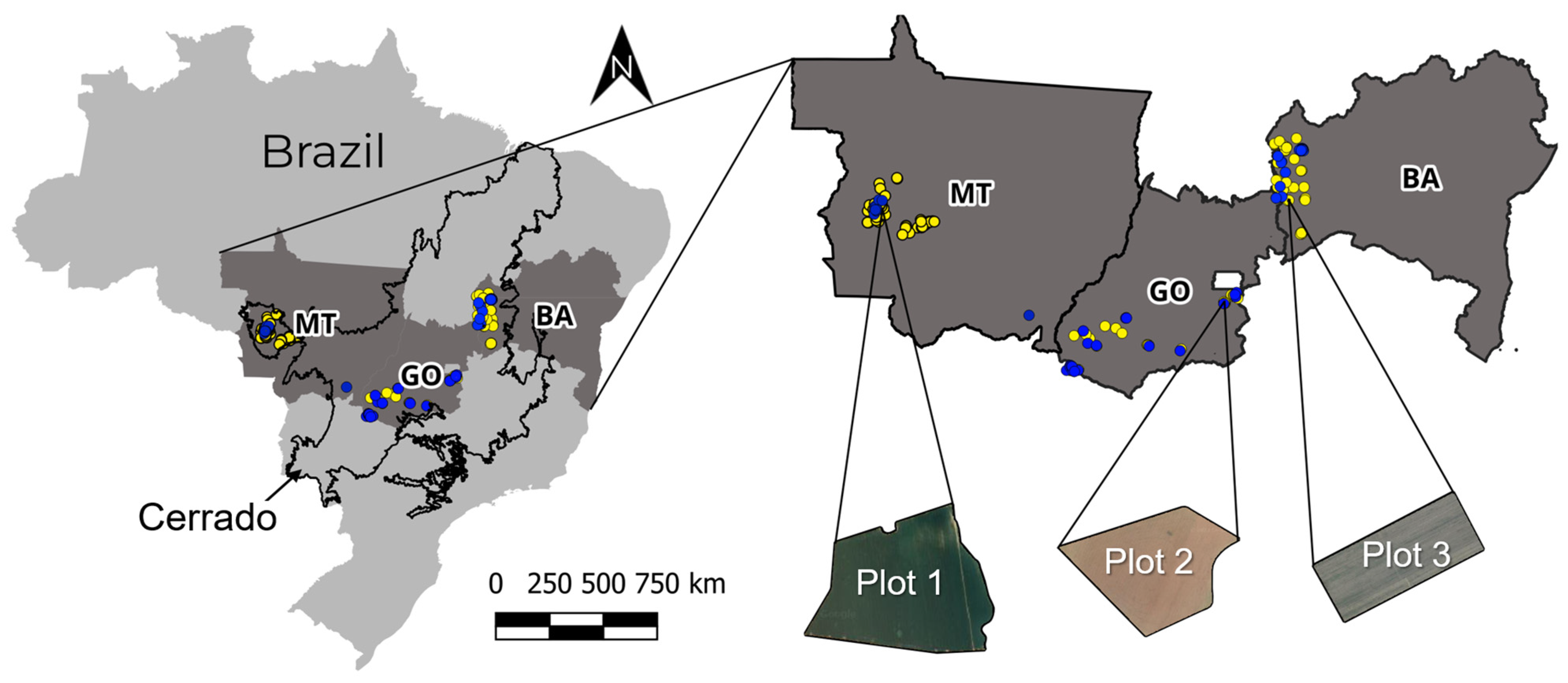
2. Materials and Methods
2.1. Experimental Areas and Dataset
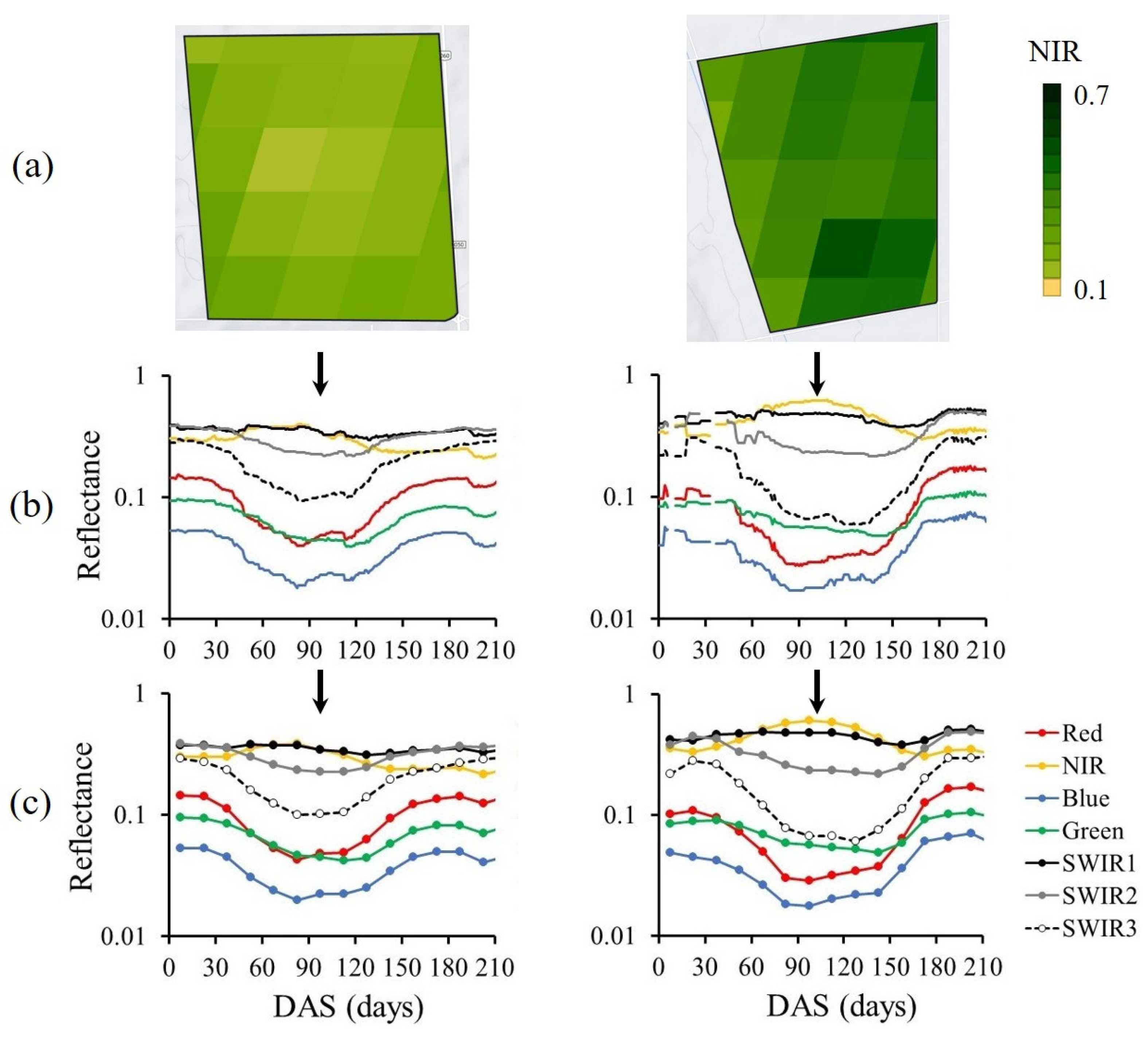
2.2. Satellite Data Acquisition and Preprocessing
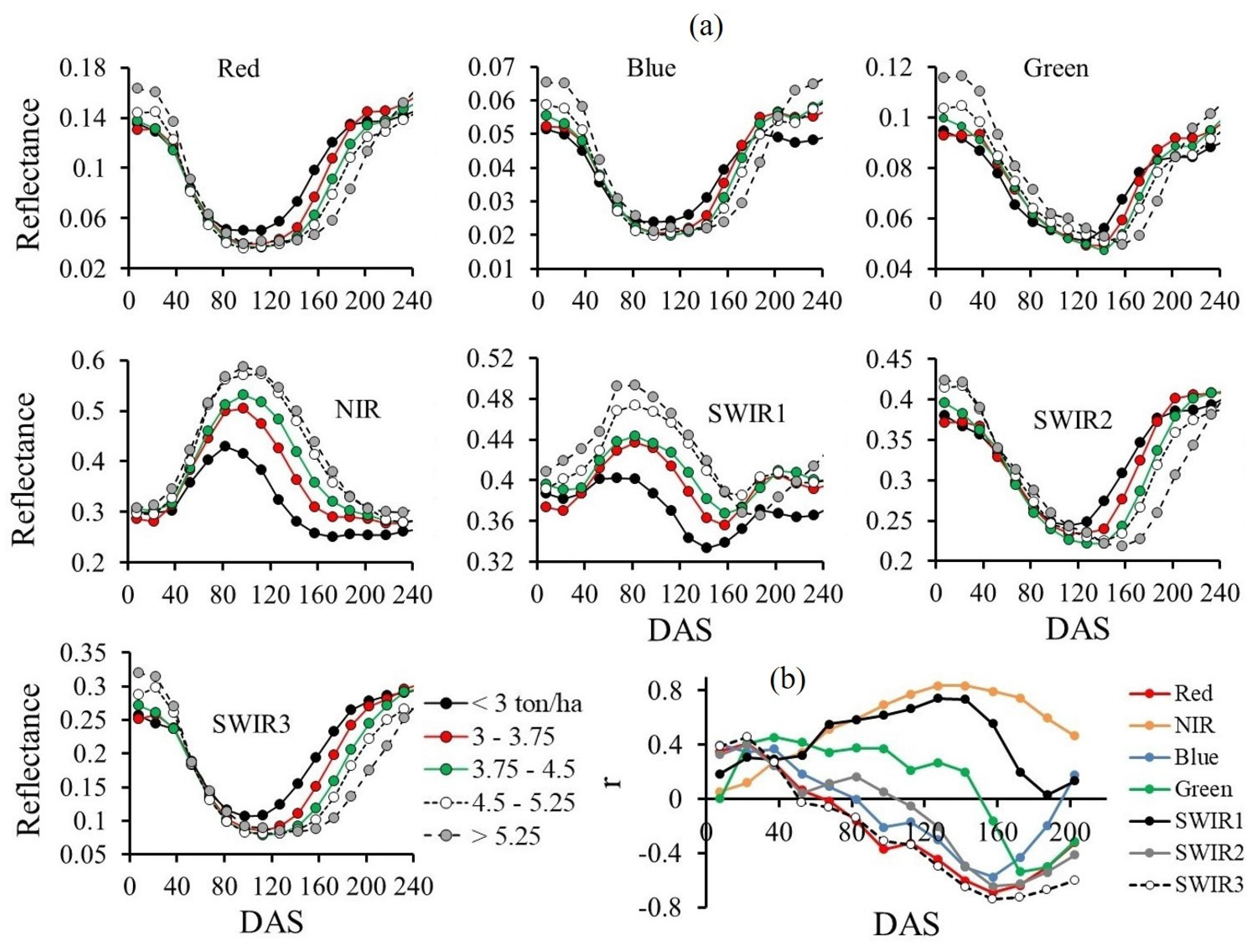
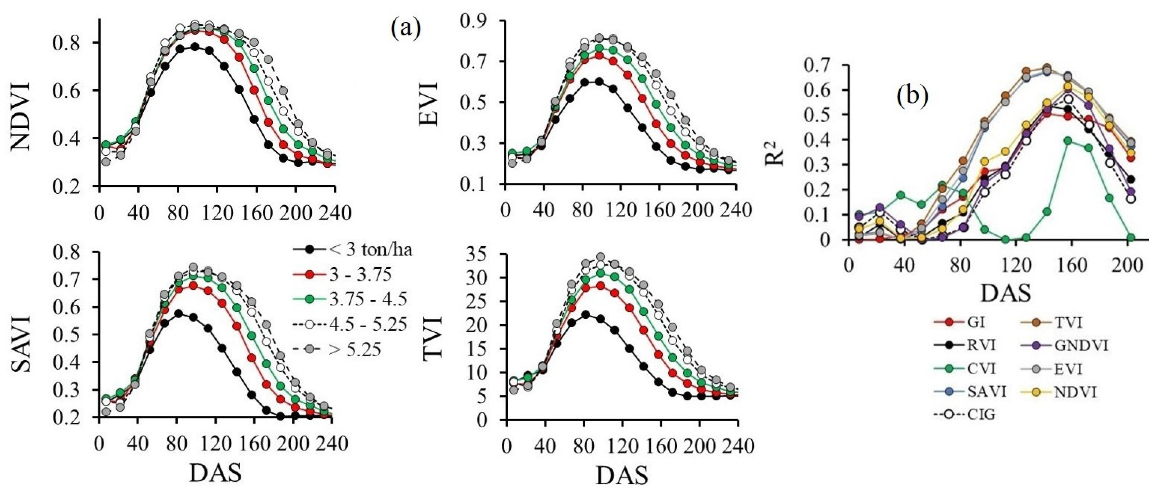
3. Results and Discussion
4. Conclusions
Author Contributions
Funding
Data Availability Statement
Conflicts of Interest
References
- ABRAPA. Safra Brasil. 2024. Available online: https://abrapa.com.br/dados/ (accessed on 16 February 2024).
- Eiten, G. Cerrado vegetation: Vegetation and climate in Brazil. In Cerrado: Characterization, Occupation and Perspectives, 2nd ed.; Pinto, M.N., Ed.; UNB: Brasília, Brazil, 1993; pp. 17–73. (In Portuguese) [Google Scholar]
- COTTON BRAZIL. Market Report, 19 January 2024. 2024. Available online: https://cottonbrazil.com/download/abrapa-cotton-brazil-report-january-2024/ (accessed on 16 February 2024).
- Echer, F.R.; Mello, P.R.; Rosolem, C.A. Management of plant growth regulators. In Best Management Practices for Cotton in Mato Grosso State, 4th ed.; Belot, J.L., Vilela, P.M.C.A., Eds.; IMAmt-AMPA: Cuiabá, Brazil, 2020; pp. 312–319. (In Portuguese) [Google Scholar]
- CONAB. Companhia Nacional de Abastecimento. 2024. Available online: https://www.conab.gov.br/info-agro/safras/serie-historica-das-safras/itemlist/category/898-algodao (accessed on 16 February 2024).
- Basso, B.; Liu, L. Seasonal crop yield forecast: Methods, applications, and accuracies. Adv. Agron. 2019, 154, 201–255. [Google Scholar]
- Li, F.; Miao, Y.; Chen, X.; Sun, Z.; Stueve, K.; Yuan, F. In-season prediction of corn grain yield through PlanetScope and Sentinel-2 images. Agronomy 2022, 12, 3176. [Google Scholar] [CrossRef]
- Khanal, S.; Kushal, K.C.; Fulton, J.P.; Shearer, S.; Ozkan, E. Remote sensing in agriculture—Accomplishments, limitations, and opportunities. Remote Sens. 2020, 12, 3783. [Google Scholar] [CrossRef]
- Taskiner, T.; Bilgen, B. Optimization models for harvest and production planning in agri-food supply chain: A systematic review. Logistics 2021, 5, 52. [Google Scholar] [CrossRef]
- Lang, P.; Zhang, L.; Huang, C.; Chen, J.; Kang, X.; Zhang, Z.; Tong, Q. Integrating environmental and satellite data to estimate county-level cotton yield in Xinjiang Province. Front. Plant Sci. 2023, 13, 1048479. [Google Scholar] [CrossRef] [PubMed]
- Prasad, N.R.; Patel, N.R.; Danodia, A. Crop yield prediction in cotton for regional level using Random Forest approach. Spat. Inf. Res. 2020, 29, 195–206. [Google Scholar] [CrossRef]
- Filippi, P.; Whelan, M.B.; Vervoort, R.W.; Bishop, T.F.A. Mid-season empirical cotton yield forecasts at fine resolutions using large yield mapping datasets and diverse spatial covariates. Agric. Syst. 2020, 184, 102894. [Google Scholar] [CrossRef]
- Meng, L.; Liu, H.; Ustin, S.L.; Zhang, X. Assessment of FSDAF accuracy on cotton yield estimation using different Modis products and Landsat based on the mixed degree index with different surroundings. Sensors 2021, 21, 5184. [Google Scholar] [CrossRef] [PubMed]
- Johnson, D.M.; Rosales, A.; Mueller, R.; Reynolds, C.; Frantz, R.; Anyamba, A.; Pak, E.; Tucker, C. USA crop yield estimation with MODIS NDVI: Are remotely sensed models better than simple trend analyses? Remote Sens. 2021, 13, 4227. [Google Scholar] [CrossRef]
- Johnson, D.M. A comprehensive assessment of the correlations between field crop yields and commonly used MODIS products. Int. J. Appl. Earth Obs. Geoinf. 2016, 52, 65–81. [Google Scholar] [CrossRef]
- Iqbal, J.; Read, J.; Whisler, D. Using remote sensing and soil physical properties for predicting the spatial distribution of cotton lint yield. Turk. J. Field Crops 2013, 18, 158–165. [Google Scholar]
- Feng, A.; Zhou, J.; Vories, E.D.; Sudduth, K.A.; Zhang, M. Yield estimation in cotton using UAV-based multi-sensor imagery. Biosyst. Eng. 2020, 193, 101–114. [Google Scholar] [CrossRef]
- Feng, A.; Zhang, M.; Sudduth, K.A.; Vories, E.D.; Zhou, J. Cotton yield estimation from UAV-based plant height. Trans. ASABE 2019, 62, 393–403. [Google Scholar] [CrossRef]
- Ballester, C.; Hornbuckle, J.; Brinkhoff, J.; Smith, J.; Quayle, W. Assessment of in-season cotton nitrogen status and lint yield prediction from Unmanned Aerial System imagery. Remote Sens. 2017, 9, 1149. [Google Scholar] [CrossRef]
- Huang, Y.; Brand, H.J.; Sui, R.; Thomson, S.J.; Furukawa, T.; Ebelhar, M.W. Cotton yield estimation using very high-resolution digital images acquired with a low-cost Small Unmanned Aerial Vehicle. Trans. ASABE 2016, 59, 1563–1574. [Google Scholar]
- Huang, Y.; Sui, R.; Thomson, J.S.; Fisher, D.K. Estimation of cotton yield with varied irrigation and nitrogen treatments using aerial multispectral imagery. Int. J. Agric. Biol. Eng. 2013, 6, 37–41. [Google Scholar]
- Zhao, D.; Reddy, K.R.; Kakani, V.G.; Read, J.J.; Koti, S. Canopy reflectance in cotton for growth assessment and lint yield prediction. Eur. J. Agron. 2007, 26, 335–344. [Google Scholar] [CrossRef]
- He, Y.; Qiu, B.; Cheng, F.; Chen, C.; Sun, Y.; Zhang, D.; Lin, L.; Xu, A. National scale maize yield Estimation by integrating multiple spectral indexes and temporal aggregation. Remote Sens. 2023, 15, 414. [Google Scholar] [CrossRef]
- Fu, Y.; Huang, J.; Shen, Y.; Liu, S.; Huang, Y.; Dong, J.; Han, W.; Ye, T.; Zhao, W.; Yuan, W. A satellite-based method for national winter wheat yield estimating in China. Remote Sens. 2021, 13, 4680. [Google Scholar] [CrossRef]
- Jeong, S.; Shin, T.; Ban, J.; Ko, K.J. Simulation of spatiotemporal variations in cotton lint yield in the Texas high plains. Remote Sens. 2022, 14, 1421. [Google Scholar] [CrossRef]
- Ashapure, A.; Jung, J.; Chang, A.; Oh, S.; Yeom, J.; Maeda, M.; Maeda, A.; Dube, N.; Landivar, J.; Hague, S.; et al. Developing a machine learning based cotton yield estimation framework using multi-temporal UAS data. ISPRS J. Photogramm. Remote Sens. 2020, 169, 180–194. [Google Scholar] [CrossRef]
- Meng, L.; Liu, H.; Zhang, X.; Ren, C.; Ustin, S.; Qiu, Z.; Xu, M.; Guo, D. Assessment of the effectiveness of spatiotemporal fusion of multi-source satellite images for cotton yield estimation. Comput. Electron. Agric. 2019, 162, 44–52. [Google Scholar] [CrossRef]
- He, L.; Mostovoy, G. Cotton yield estimate using Sentinel-2 data and an ecosystem model over the southern US. Remote Sens. 2019, 11, 2000. [Google Scholar] [CrossRef]
- Baio, F.H.R.; da Silva, E.E.; Martins, P.H.A.; da Silva-Júnior, C.A.; Teodoro, P.E. In situ remote sensing as a strategy to predict cotton seed yield. J. Biosci. 2019, 35, 1847–1854. [Google Scholar] [CrossRef]
- Haghverdi, A.; Washington-Allen, R.A.; Leib, B.G. Prediction of cotton lint yield from phenology of crop indices using artificial neural networks. Comput. Electron. Agric. 2018, 152, 186–197. [Google Scholar] [CrossRef]
- Meng, L.; Zhang, X.; Huanjun, L.; Guo, D.; Yan, Y.; Qin, L.; Pan, Y. Estimation of cotton yield using the reconstructed time-series vegetation index of Landsat data. Can. J. Remote Sens. 2017, 43, 244–255. [Google Scholar] [CrossRef]
- Galbieri, R.; Vaz, C.M.P.; Pessatto-Filho, D.; Crestana, S.; Chitarra, L.G.; Lobo-Junior, M.; Lanças, F.M.; Silva, J.F.V.; Faleiro, V.O.; Sarques, B. Cotton Production in Goiás: White Mold, Fusarium Wilt, Cultivation System and Soil Physical Attributes; Circular Técnica; AGOPA: Goiânia, Brazil, 2018; 20p. (In Portuguese) [Google Scholar]
- Galbieri, R.; Vaz, C.M.P.; Silva, J.F.V.; Amus, G.L.A.; Crestana, S.; Matos, E.S.; Magalhaes, C.A.S. Influence of soil parameters on the occurrence of phytonematodes. In Phytoparasitic Nematodes of Cotton in Brazilian Cerrados: Biology and Control Measures, 1st ed.; Galbieri, R., Belot, J.L., Eds.; IMAmt: Cuiabá, Brazil, 2016; pp. 37–90. (In Portuguese) [Google Scholar]
- Perina, F.J.; Bogiani, J.C.; Ribeiro, G.C.; Breda, C.E.; Fabris, A.; dos Santos, I.A.; Seibel, D.P. Survey and Management of Phytonematodes in Cotton in Western Bahia, Results for Season 2016/17; Circular Técnica; Fundação: Bahia, Brazil, 2017; 8p. [Google Scholar]
- INMET—Instituto Nacional de Meteorologia. Boletim de Monitoramento Agrícola—Culturas de Verão 21/22, 11(5):1-19. 2022. Available online: https://portal.inmet.gov.br/ (accessed on 16 February 2024).
- AGRITEMPO. Agrometeorological Monitoring System. 2024. Available online: http://www.agritempo.gov.br/agritempo/sobre.jsp?lang=en (accessed on 16 February 2024).
- QGIS Development Team. QGIS Geographic Information System. Open Source Geospatial Foundation Project. 2022. Available online: http://qgis.osgeo.org (accessed on 16 February 2024).
- MODIS. Moderate Resolution Imaging Spectroradiometer. 2024. Available online: https://modis.gsfc.nasa.gov/ (accessed on 21 March 2024).
- GEE—Google Earth Engine. 2024. Available online: https://earthengine.google.com/platform/ (accessed on 21 March 2024).
- Gitelson, A.A.; Gritz, Y.; Merzlyak, M.N. Relationships between leaf chlorophyll content and spectral reflectance and algorithms for non-destructive chlorophyll assessment in higher plant leaves. J. Plant Physiol. 2003, 160, 271–282. [Google Scholar] [CrossRef] [PubMed]
- Jordan, C.F. Derivation of leaf-area index from quality of light on the forest floor. Ecology 1969, 50, 663–666. [Google Scholar] [CrossRef]
- Vincini, M.; Frazzi, E.; D’Alessio, P. A broad-band leaf chlorophyll vegetation index at the canopy scale. Precis. Agric. 2008, 9, 303–319. [Google Scholar] [CrossRef]
- Huete, A.R. A soil-adjusted vegetation index (SAVI). Remote Sens. Environ. 1988, 25, 295–309. [Google Scholar] [CrossRef]
- Broge, N.H.; Leblanc, E. Comparing prediction power and stability of broadband and hyperspectral vegetation indices for estimation of green leaf area index and canopy chlorophyll density. Remote Sens. Environ. 2001, 76, 156–172. [Google Scholar] [CrossRef]
- Kaufman, Y.J.; Merzlyak, M.N. Use of a green channel in remote sensing of global vegetation from EOS-MODIS. Remote Sens. Environ. 1996, 58, 289–298. [Google Scholar]
- Huete, A.; Didan, K.; Miura, T.; Rodriguez, E.P.; Gao, X.; Ferreira, L.G. Overview of the radiometric and biophysical performance of the MODIS vegetation indices. Remote Sens. Environ. 2002, 83, 195–213. [Google Scholar] [CrossRef]
- Rouse, J.W. Monitoring vegetation systems in the great plains with ERTS. In Proceedings of the Third Earth Resources Technology Satellite-1 Symposium—Volume I: Technical Presentations; Goddard Space Flight Center NASA SP-351; NASA: Washington, DC, USA, 1974; Paper A-20; pp. 309–317. [Google Scholar]
- Chattopadhyay, N.; Shukla, K.K.; Birah, A.; Khokhar, M.K.; Kanojia, A.K.; Nigam, R.; Roy, A.; Bhattacharya, B.K. Identification of spectral bands to discriminate wheat Spot Blotch using in situ hyperspectral data. J. Indian Soc. Remote Sens. 2023, 51, 917–934. [Google Scholar] [CrossRef]
- Knipling, E.B. Physical and physiological basis for the reflectance of visible and near-infrared radiation from vegetation. Remote Sens. Environ. 1970, 1, 155–159. [Google Scholar] [CrossRef]
- Thenkabail, P.S.; Smith, R.B.; De Pauw, E. Hyperspectral vegetation indices and their relationships with agricultural crop characteristics. Remote Sens. Environ. 2000, 71, 158–182. [Google Scholar] [CrossRef]
- Tesfaye, A.A.; Awoke, B.G. Evaluation of the saturation property of vegetation indices derived from sentinel-2 in mixed crop-forest ecosystem. Spat. Inf. Res. 2020, 1, 109–121. [Google Scholar]
- Xing, N.; Huang, W.; Xie, Q.; Shi, Y.; Ye, H.; Dong, Y.; Wu, M.; Sun, G.; Jiao, Q. A transformed triangular vegetation index for estimating winter wheat leaf area index. Remote Sens. 2020, 12, 16. [Google Scholar] [CrossRef]
- Shammi, S.A.; Meng, Q. Use time series NDVI and EVI to develop dynamic crop growth metrics for yield modeling. Ecol. Indic. 2021, 121, 107124. [Google Scholar] [CrossRef]
- Carvalho, M.C.S.; Ferreira, G.B. Cotton Liming and Fertilization in the Cerrado; Circular Técnica 92; Embrapa: Campina Grande, Brazil, 2006; 16p. (In Portuguese) [Google Scholar]


| Vegetation Indices | Formulation | Reference |
|---|---|---|
| Green Index (GI) | GI = G/R | [40] |
| Ratio Vegetation Index (RVI) | RVI = NIR/R | [41] |
| Chlorophyll Vegetation Index (CVI) | CVI = (NIR × R)/G2 | [42] |
| Soil-Adjusted Vegetation Index (SAVI) | SAVI = 1.5 × (NIR − R)/(0.5 × NIR + R) | [43] |
| Chlorophyll index—green (CIG) | CIG = (NIR/G) − 1 | [40] |
| Triangular Chlorophyll Absorption Ratio Index (TVI) | TVI = 60 × NIR − G − 100 × (R – G) | [44] |
| Green NDVI (GNDVI) | GNDVI = (NIR − G)/(NIR + G) | [45] |
| Enhanced Vegetation Index (EVI) | EVI = 2.5 × (NIR − R)/(1 + NIR + 6 × R − 7.5 × B) | [46] |
| Normalized Differential Vegetation Index (NDVI) | NDVI = (NIR − R)/(NIR + R) | [47] |
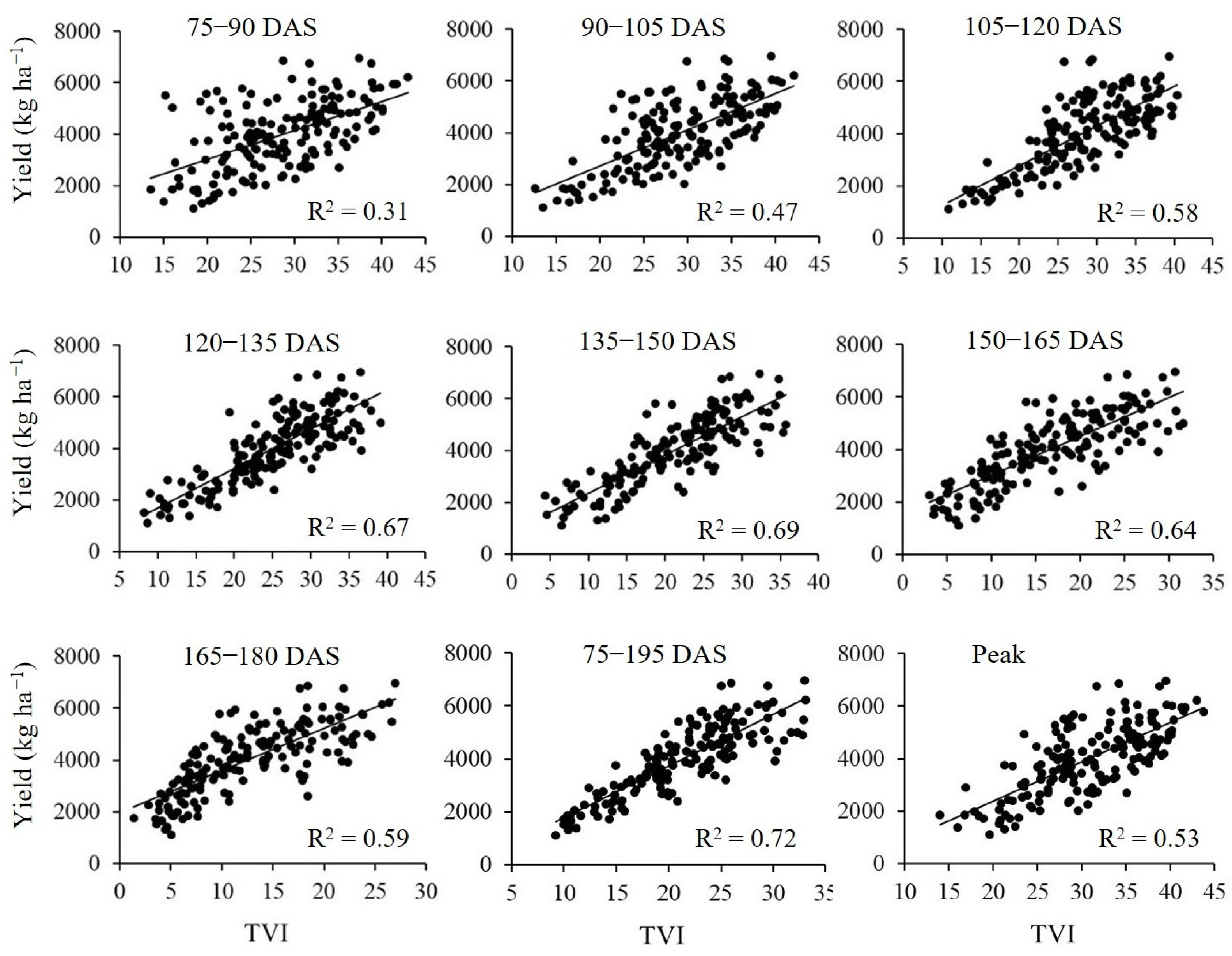
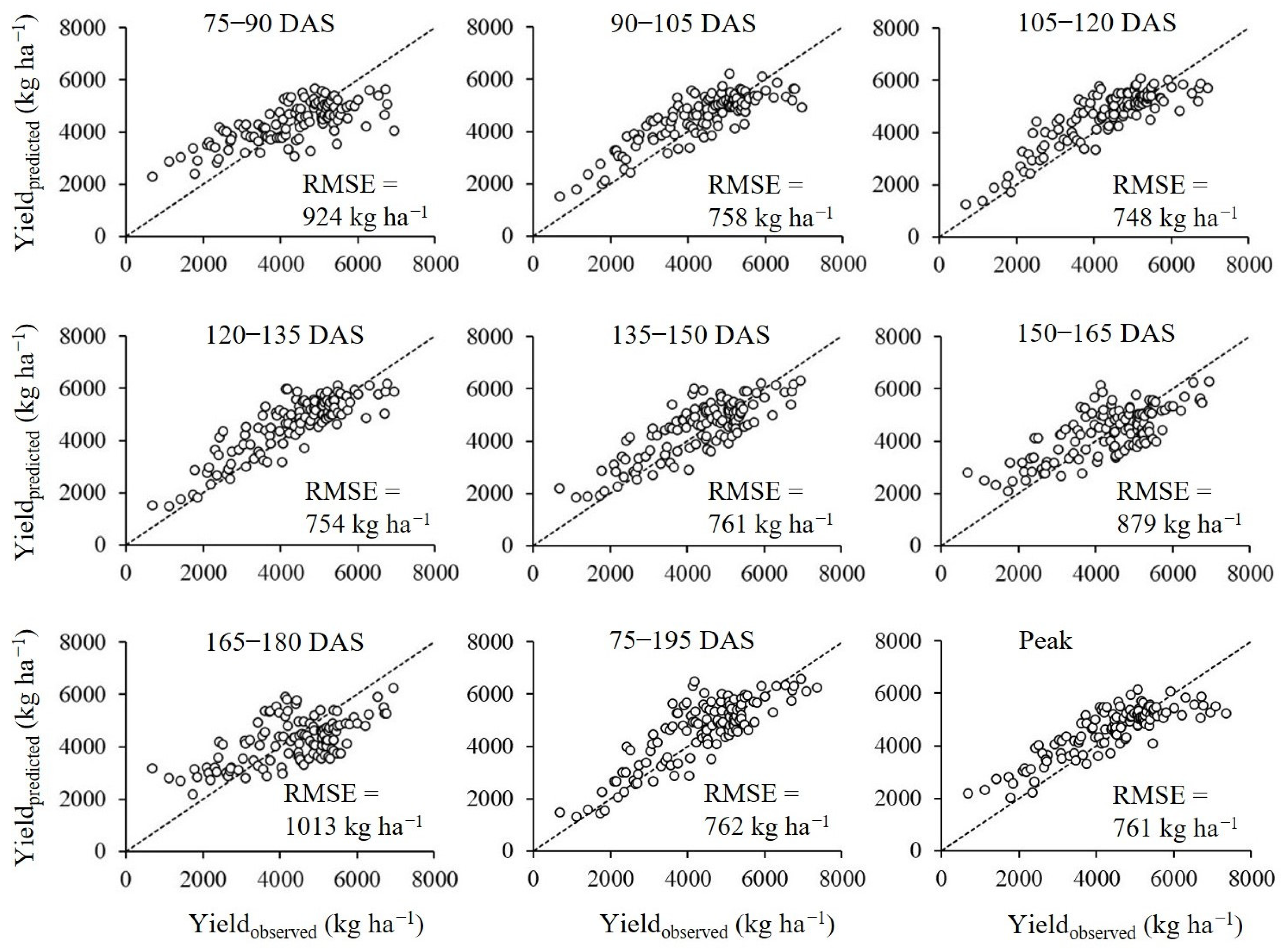
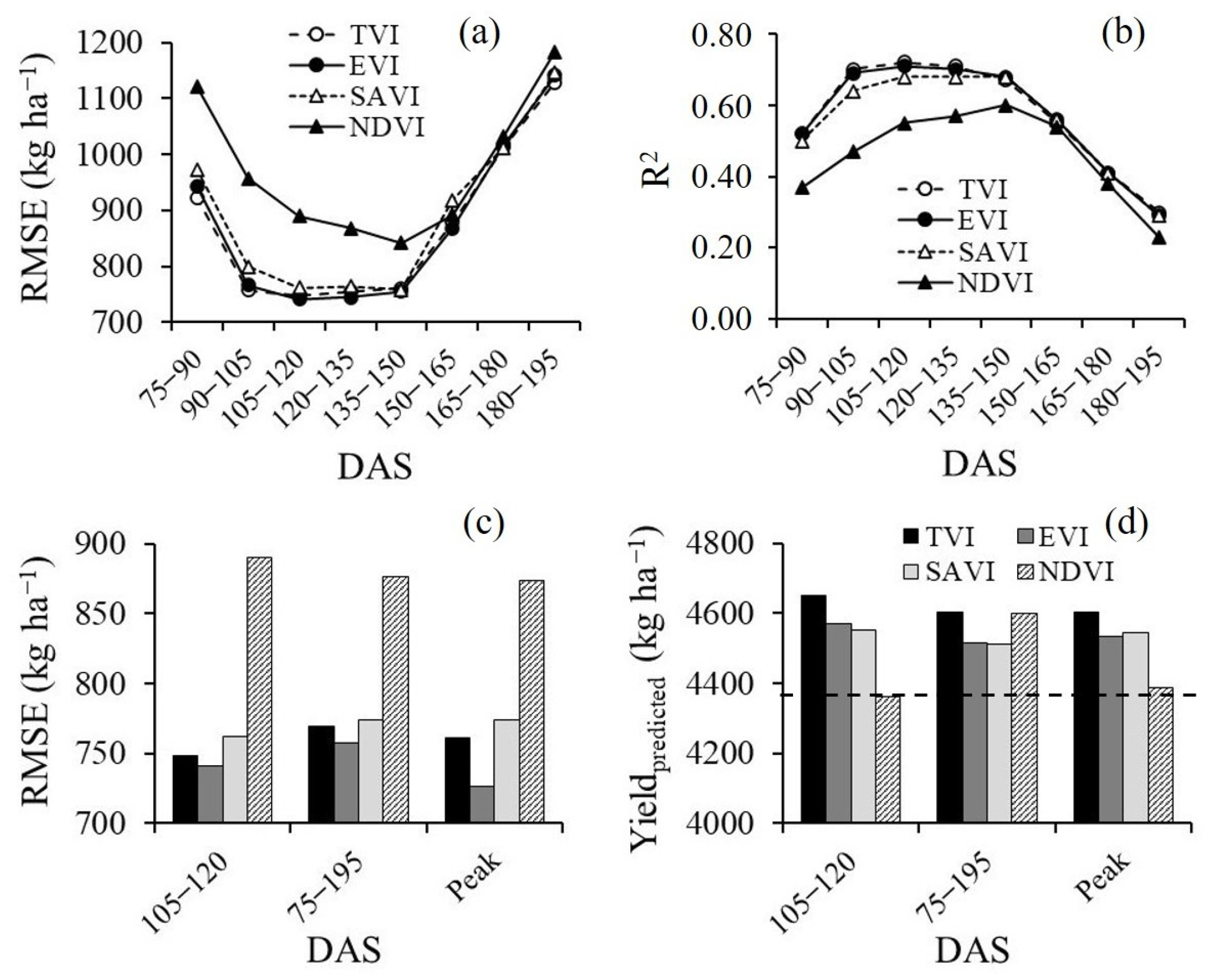
| DAS | Linear Model (TVI) | R2 | RMSE | p-Value | DAS | Linear Model (EVI) | R2 | RMSE | p-Value |
|---|---|---|---|---|---|---|---|---|---|
| kg ha−1 | (α = 0.05) | kg ha−1 | (α = 0.05) | ||||||
| 75–90 | Y = 111.96 TVI + 794.22 | 0.31 | 1088 | 3.3 × 10⁻¹⁵ | 75–90 | Y = 5133.1 EVI + 315.9 | 0.28 | 1119 | 4.1 × 10⁻¹³ |
| 90–105 | Y = 139.78 TVI − 90.918 | 0.47 | 953 | 9.5 × 10⁻²⁵ | 90–105 | Y = 6863.1 EVI − 1066.8 | 0.46 | 966 | 9.0 × 10⁻²⁴ |
| 105–120 | Y = 152.11 TVI − 269.52 | 0.58 | 856 | 1.7 × 10⁻³² | 105–120 | Y = 7316.1 EVI − 1249.5 | 0.55 | 879 | 1.4 × 10⁻³⁰ |
| 120–135 | Y = 152.87TVI + 166.22 | 0.67 | 752 | 7.6 × 10−42 | 120–135 | Y = 7013.0 EVI − 608.5 | 0.65 | 778 | 2.3 × 10−39 |
| 135–150 | Y = 148.0 TVI + 878.89 | 0.69 | 735 | 1.8 × 10−43 | 135–150 | Y = 6484.9 EVI + 292.1 | 0.68 | 778 | 2.7 × 10−42 |
| 150–165 | Y = 147.88 TVI + 1553.7 | 0.64 | 783 | 6.5 × 10−39 | 150–165 | Y = 6170.2 EVI + 1127.9 | 0.65 | 776 | 1.5 × 10−39 |
| 165–180 | Y = 162.65 TVI + 1957.8 | 0.59 | 843 | 1.4 × 10⁻³³ | 165–180 | Y = 6456.5 EVI + 1636.5 | 0.59 | 842 | 1.1 × 10⁻³³ |
| 180–195 | Y = 195.06 TVI + 2130.5 | 0.49 | 941 | 1.1 × 10⁻²⁵ | 180–195 | Y = 7602.2 EVI + 1801.6 | 0.48 | 947 | 3.2 × 10⁻²⁵ |
| 75–195 | Y = 196.28 TVI − 189.77 | 0.72 | 690 | 5.9 × 10−48 | 75–195 | Y = 8891.9 EVI − 1026.2 | 0.73 | 688 | 3.9 × 10−48 |
| Peak | Y = 150.52 TVI − 634.87 | 0.53 | 900 | 7.4 × 10⁻²⁹ | Peak | Y = 7813.9 EVI − 1996.1 | 0.53 | 901 | 8.4 × 10⁻²⁹ |
| DAS | Linear Model (SAVI) | R2 | RMSE | p-value | DAS | Linear Model (NDVI) | R2 | RMSE | p-value |
| kg ha−1 | (α = 0.05) | kg ha−1 | (α = 0.05) | ||||||
| 75–90 | Y = 6804.1 SAVI − 543.3 | 0.25 | 1140 | 8.2 × 10⁻¹² | 75–90 | Y = 6111.6 NDVI − 1057.4 | 0.12 | 1232 | 4.5 × 10⁻⁶ |
| 90–105 | Y = 9495.4 SAVI − 2479.4 | 0.45 | 977 | 5.8 × 10⁻²³ | 90–105 | Y = 11,059 NDVI − 5334.6 | 0.31 | 1089 | 4.3 × 10⁻¹⁵ |
| 105–120 | Y = 10,008 SAVI − 2696 | 0.55 | 1132 | 6.1 × 10⁻³⁰ | 105–120 | Y = 11,093 NDVI − 5287.1 | 0.35 | 1058 | 3.3 × 10⁻¹⁷ |
| 120–135 | Y = 9164.3 SAVI − 1712.5 | 0.64 | 784 | 8.2 × 10−39 | 120–135 | Y = 9500.8 NDVI − 3674.2 | 0.46 | 966 | 8.7 × 10⁻²⁴ |
| 135–150 | Y = 7937.6 SAVI − 415.88 | 0.67 | 753 | 9.7 × 10−42 | 135–150 | Y = 7473.6 NDVI − 1618 | 0.55 | 884 | 3.6 × 10⁻³⁰ |
| 150–165 | Y = 7729.7 SAVI + 624.53 | 0.66 | 809 | 5.6 × 10−40 | 150–165 | Y = 6243.6 NDVI − 80.36 | 0.61 | 816 | 6.0 × 10−36 |
| 165–180 | Y = 7244.4 SAVI + 1251.7 | 0.59 | 840 | 7.9 × 10⁻³⁴ | 165–180 | Y = 5550.8 NDVI + 1002 | 0.57 | 861 | 4.8 × 10⁻³² |
| 180–195 | Y = 8316.9 SAVI + 1422.3 | 0.47 | 952 | 7.5 × 10⁻²⁵ | 180–195 | Y = 5922.8 NDVI + 1386.4 | 0.46 | 970 | 1.6 × 10⁻²³ |
| 75–195 | Y = 11,152 SAVI − 2066.5 | 0.73 | 688 | 1.9 × 10−48 | 75–195 | Y = 11,230 NDVI + 4003.9 | 0.67 | 752 | 8.1 × 10−42 |
| Peak | Y = 11,044.7 SAVI − 3770 | 0.51 | 919 | 2.3 × 10⁻²⁷ | Peak | Y = 15,470 NDVI − 9131.6 | 0.39 | 1029 | 3.2 × 10⁻¹⁹ |
| Reference | RS | DAS | Reference | RS | DAS |
|---|---|---|---|---|---|
| [19] | UAV | 150–170 | [27] | Satellite | 100 |
| [30] | Satellite | 90–160 | [26] | UAV | 90–100 |
| [10] | Satellite | 90–150 | [12] | Satellite | 90 * |
| [15] | Satellite | 120 | [31] | Satellite | 80–90 |
| [21] | Airborne | 115 * | [18] | UAV | 80 * |
| [17] | UAV | 90–120 | [29] | Active Sensor | 60–100 |
| [16] | Satellite | 105 | [22] | Spectroradiometer | 75 |
Disclaimer/Publisher’s Note: The statements, opinions and data contained in all publications are solely those of the individual author(s) and contributor(s) and not of MDPI and/or the editor(s). MDPI and/or the editor(s) disclaim responsibility for any injury to people or property resulting from any ideas, methods, instructions or products referred to in the content. |
© 2024 by the authors. Licensee MDPI, Basel, Switzerland. This article is an open access article distributed under the terms and conditions of the Creative Commons Attribution (CC BY) license (https://creativecommons.org/licenses/by/4.0/).
Share and Cite
de Siqueira, D.A.B.; Vaz, C.M.P.; da Silva, F.S.; Ferreira, E.J.; Speranza, E.A.; Franchini, J.C.; Galbieri, R.; Belot, J.L.; de Souza, M.; Perina, F.J.; et al. Estimating Cotton Yield in the Brazilian Cerrado Using Linear Regression Models from MODIS Vegetation Index Time Series. AgriEngineering 2024, 6, 947-961. https://doi.org/10.3390/agriengineering6020054
de Siqueira DAB, Vaz CMP, da Silva FS, Ferreira EJ, Speranza EA, Franchini JC, Galbieri R, Belot JL, de Souza M, Perina FJ, et al. Estimating Cotton Yield in the Brazilian Cerrado Using Linear Regression Models from MODIS Vegetation Index Time Series. AgriEngineering. 2024; 6(2):947-961. https://doi.org/10.3390/agriengineering6020054
Chicago/Turabian Stylede Siqueira, Daniel A. B., Carlos M. P. Vaz, Flávio S. da Silva, Ednaldo J. Ferreira, Eduardo A. Speranza, Júlio C. Franchini, Rafael Galbieri, Jean L. Belot, Márcio de Souza, Fabiano J. Perina, and et al. 2024. "Estimating Cotton Yield in the Brazilian Cerrado Using Linear Regression Models from MODIS Vegetation Index Time Series" AgriEngineering 6, no. 2: 947-961. https://doi.org/10.3390/agriengineering6020054