Some Geospatial Insights on Orange Grove Site Selection in a Portion of the Northern Citrus Belt of Mexico

Abstract

This study aimed to delineate the most suitable areas for sustainable citrus production by integrating multi-criteria decision analysis, time-series remote sensing, and principal component analysis in a portion of the northern citrus belt of Mexico, particularly in the Rioverde Valley. Fourteen specific factors were grouped into four main factors, i.e., topography, soil, climate, and proximity to water sources, to carry out a multi-criteria decision analysis for classifying production areas according to suitability levels. To explore the effect of precipitation on land suitability for citrus production, we analyzed the historical record of annual precipitation estimated by processing 20-year NDVI daily data. The multi-criteria model was run for every precipitation year. The final map of land suitability was obtained by using the first component after principal component analysis on annual land suitability maps. The results indicate that approximately 30% of the study area is suitable for growing orange groves, with specific areas designated as suitable based on both mean annual precipitation (MAP) and principal component analysis (PCA) criteria, resulting in 84,415.7 ha and 95,485.5 ha of suitable land, respectively. The study highlighted the importance of remotely sensed data-based time-series precipitation in predicting potential land suitability for growing orange groves in semiarid lands. Our results may support decision-making processes for the effective land management of orange groves in the Mexico’s Rioverde region.

1. Introduction

Mexico is the fifth most important orange producing country in the world, after Brazil, the United States, China and India. Mexican orange production is mainly distributed across four states, including Veracruz, Tamaulipas, San Luis Potosí, and Nuevo León. Particularly in the state of San Luis Potosí, the Rioverde region produces quality oranges, which gives it a high value in the market [1]. During 2020 and 2021, San Luis Potosí exhibited a production of approximately 376,613 t of oranges (Citrus sinensis); and in particular, the Rioverde region (including the municipality of Rioverde and Ciudad Fernández) produced 120,000 t on a sown area of 5650 ha, that is, approximately 30% of orange production for the whole state, positioning the Rioverde region as an important place regarding citrus production in the state of San Luis Potosí [2].

Mexico’s orange production has faced several constraints over the past decade, including water scarcity, diseases, and land use change. Orange production relies heavily on groundwater from wells, which are recharged by precipitation. A recent drought, however, resulting in decreased rainfall, has posed a threat to orange production in the study area [3,4]. The rainfall normally ranged between 375 and 604 mm annually [5] but now is currently showing an entirely different pattern. According to information provided by CONAGUA’s National Meteorological System (SMN), the average rainfall has been between 300 and 400 mm per year in the study area in recent years [6]. Therefore, water scarcity, mainly due to precipitation anomalies [7,8,9], has led to pest and disease problems [10]. Additionally, other causes exist for the diminishing orange grove area, including land use change mainly driven by urban growth. Urban growth engulfs orange groves for a number of reasons: (1) a lack of profitability in orange production caused by crop diseases, leading to decisions to sell the land to urban developers; (2) orange groves are inherited by heirs, but they do not want to be farmers; therefore, they themselves also decide to sell their land property; and (3) the same family decides to build inside the grove [11].

Citrus trees are adaptable to various soils, but their shallow root system and limited root hairs make nutrient absorption challenging. Soil characteristics are vital for cultivation. Citrus trees thrive in light soils like sandy loam, loam, or clay loam, with good drainage and aeration. Heavy or clayey soils with poor drainage are unsuitable and can lead to growth issues and root diseases. Citrus trees can tolerate a pH range of 4 to 9, but the optimal pH is 5.5 to 6. They can handle up to 30% acidity saturation, but aluminum saturation should not exceed 20%. Citrus trees can still grow in soils with a pH above 7, as long as salt or sodium accumulation is not a problem. In such conditions, monitoring micronutrient deficiencies is mandatory, as they can significantly impact yield [12].

Geographic information systems have been used to assess the suitability of land for crop production. Selecting potential locations for establishing new fruit orchards is an important issue for planning future land use toward sustainable agriculture [13]. A widely used method for mapping land suitability is the so-called multi-criteria decision analysis (MCDA). This method has been used to solve complex problems combining numerous variables at different levels of interaction [14,15]. Some agricultural applications of MCDA in agriculture can be found in recent the literature, i.e., land suitability for tea crops [16], Eragrostis tef for flour production in bread-making [17], land suitability for wheat [18], land suitability for barley production [19], rice production [20], land suitability for wheat and maize [21], land suitability for maize [22], and land suitability for Moringa oleifera [23].

In particular, for citrus crops, Elsheikh et al. [24] developed a tool for assessing the suitability of agricultural land for planning tropical and subtropical crops, including citrus in Malaysia. Zabihi et al. [25] mapped land suitability for sustainable citrus planning in a northern region of Iran using the analytical network process (ANP) within a GIS environment. Mokarram and Mirsoleimani [26] mapped land suitability for citrus crops in the province of Fars, Iran, using multi-criteria decision analysis. Tercan and Dereli [27] developed a land suitability model for citrus cultivation in the Mediterranean region of Turkey. Orhan [28] determined land suitability for citrus cultivation using MCDA in Mersin, Turkey. Although the studies mentioned above have made significant contributions to the use of MCDA in the context of citrus crops, our motivation was to assess biophysical factors, e.g., interannual rainfall estimated with remotely sensed data, possibly related to land suitability for citrus cultivation.

Principal component analysis (PCA) is a multivariate technique for data dimension reduction used in multiple fields of study [29]. In the context of spatial science, PCA may be used spatially and temporally. When used spatially, this technique can be applied to highlight spectral features on remotely sensed data, e.g., in a single-date satellite scene, PCA can fuse spectral bands into new principal components that capture biophysical features such as chlorophyll (greenness) and moisture (wetness) [30]. Researchers have created RGB-composite imagery with the three first principal components to emphasize the spectral characteristics of natural cover [31]; others have used PCA as a noise-detection technique [32], and moreover, others have used it as a denoising technique [33]. When used temporally, this technique can be employed in time-series data for analyzing temporal patterns of a single variable, e.g., NDVI. In this case, the first principal component assimilates all the whole radiometric behavior that is common throughout the time series. The second principal component incorporates characteristics not included in the first principal component and is interpreted as a component for change analysis [34,35].

Time-series analysis of remotely sensed data has been conducted using both desktop mapping and cloud computing analysis, such as Google Earth Engine. In the case of Mexico, there have been limited studies on the use of time-series remotely sensed data to monitor environmental biophysical variables using vegetation indexes as proxies. Noteworthy works by Colditz et al. have focused on studying phenology [36], land use changes [37], and NDVI trends [38] in Mexico based on time-series remotely sensed data. However, for the state of San Luis Potosí, research on the analysis of the Normalized Difference Vegetation Index (NDVI) was carried out until 2012 [35]. In this study, MODIS time series data from 2000 to 2010 were employed, with a spatial resolution of 500 m, revealing dry conditions from 2000 to 2005 and wet conditions from 2006 to 2010. Additionally, these researchers developed a nonlinear model to predict annual precipitation based on NDVI maxima. All these methodological advantages of remote sensing research in the study area have amalgamated a number of conditions to the use of use of remotely sensed data to predict annual precipitation using remotely sensed data for a long-time data series of NDVI trend, in order to have a spatiotemporal estimation of precipitation.

Otherwise, precision agriculture in semiarid lands is challenging [39]. Farmers are required to tackle water scarcity when producing specialty crops to supply local and external demand for food products [40]. Remote sensing plays a key role when monitoring environmental variables, i.e., precipitation, for agricultural production in semiarid lands [41]. Particularly, spectral indices built by using remotely sensed time-series data may be used as a proxy for precipitation monitoring [35,42]. As an authentic concern on the continuity of growing orange groves in the Rioverde region, this research was designed to investigate the status of land suitability for orange grove cultivation under a spatiotemporal perspective using 20-year remotely sensed time-series data as a proxy for precipitation in the context of the MCDA approach by combining different criteria, including topography, soil, climate, and proximity factors, in the Mexico’s Rioverde region. Therefore, we hypothesize that spatiotemporal shifts in land suitability can be elucidated through the examination of precipitation variations, inferred from remotely sensed data. Consequently, this study seeks to evaluate how these inferred precipitation variations have influenced the overall suitability of land for orange grove cultivation, emphasizing their role alongside multiple criteria such as topography, soil properties, climate conditions, and proximity to water sources.

2. Materials and Methods

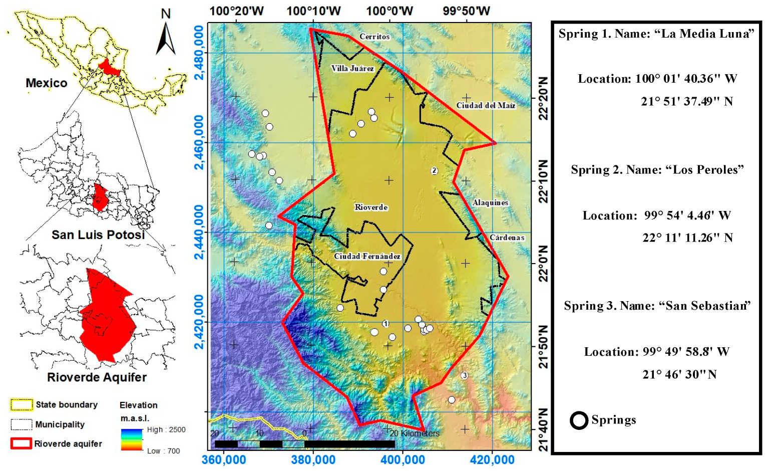
2.1. Study Area

This study was conducted in a portion of Mexico’s citrus production belt, particularly in the Rioverde region in the middle zone of the state of San Luis Potosí. The study area was located within the political–administrative boundaries of the Rioverde aquifer, which is delimited between the meridians 100°15′36.19″ W and 99°44′52″ W and the parallels 22°29′35″ and 21°38′12″ N (Figure 1), covering an area of 2782.66 km². This aquifer is granular, and its dynamics highly depend on the abundance of annual rainfall [43]. More than 80% of orange production in the Rioverde region depends on groundwater obtained from wells. In 2015 and 2020, the Rioverde aquifer exhibited annual water availability of 78,842,614 m³ and 29,582,580 m³, respectively [44,45], as evidence of groundwater depletion.

The study area is mostly plain with average elevations of approximately 1000 m above sea level; in the southwest direction, however, some mountains emerge with elevations ranging from 900 to 2170 m above sea level [46]. The climate is dry steppe in the northern lowlands; toward the southwest, environmental moisture increases gradually, becoming rainy temperate. The average annual temperature is 21.5 °C. Rainfall normally occurs in the summer, with an average annual rainfall of 484 mm. The temperature can reach up to 40 °C in the spring and summer, and the winter is usually cool [47].

The Rioverde valley is covered by approximately 18 springs [48], which supply water for human activities, including agriculture and urban consumption. Some of them are the origin of small water bodies that are visited by tourists, e.g., the spring known as “La Media Luna” located at 100°01′40.36″ W, 21°51′37.49″ N, the spring known as “Los Peroles” located at 99°54′3.6″ W, 22°11′13.2″ N, and the spring known as “San Sebastian” located at 99°49′58.8″ W, 21°46′30″ N, among others. Groundwater in the northern part of the Rioverde aquifer is typically characterized by high levels of calcium sulfate and calcium bicarbonate, which can result in lower quality water that may not be suitable for drinking or other purposes. However, in the southern region of the aquifer, the water quality is generally higher, and the groundwater is often considered potable or safe for human consumption [5].

2.2. Data

The spatial datasets used for carrying out the land suitability analysis for growing orange groves in the Rioverde region are presented in Figure 2. We built four main criteria using 14 subcriteria. The main criteria were as follows: topography, soil, climate, and proximity to water sources. The topography criterion comprised three subcriteria, including elevation, slope and aspect. The soil criterion consisted of the subcriteria pH, soil depth, electrical conductivity, and soil texture. The climate criteria were built with relative humidity, precipitation, mean minimum temperature, and mean maximum temperature. The proximity to water sources criterion collected the spatial variability in the distance to rivers and streams, distance to springs and distance to wells.

The topography criterion was considered by using a digital elevation model at 15 m spatial resolution obtained from the National Institute of Statistics and Geography of Mexico [46]. Slope and aspect were obtained by processing the digital elevation model using a geographic information system.

The soil criterion was built using the national soil map. The soil maps used were San Luis Potosí (F14-4), Ciudad Mante (F14-5), Guanajuato (F14-7), and Ciudad Valles (F14-8) [49,50,51,52], and for quantitative soil variables, we used the national database of soil profiles, which includes nearly 4418 data points on soil characteristics [53]. The dataset provides comprehensive environmental data, encompassing site features like vegetation, geology, temperature, precipitation, altitude, and physical and chemical analyses. We extracted 42-data points from the database, which corresponded to the spatial extent of our study area. Subsequently, we utilized these data points to construct spatial datasets for soil depth, pH, and electrical conductivity. This construction was achieved through the application of the inverse distance weighting algorithm, employing the 12 nearest neighbors and utilizing a 15 m spatial resolution as our digital elevation model [54]. All variables used for interpolation were previously averaged across all layers in the soil profile.

With regard to the climate criterion, the relative humidity was built with data gathered within a period from 1961 to 1990 by the Climatic Research Unit of the University of East Anglia [55]. The mean minimum and maximum temperatures were derived from climate normal data spanning the period from 1991 to 2020. These data were collected from 33 meteorological stations operated by the National Meteorological Service [6]. Such climate stations include data collected during a period longer than 50 years. Relative humidity and mean minimum and mean maximum temperature point data were interpolated using the inverse distance weighting algorithm specifying 12 nearest neighbors and 15 m spatial resolution [56]. Precipitation was obtained by using remotely sensed time-series data. To do this, daily MCD43A4 MODIS product data were downloaded from the Earth Data Search platform (https://search.earthdata.nasa.gov/) (accessed on 15 July 2021) for the period of 24 February 2000 to 31 December 2019, totaling 20 years of remote sensing daily observations. MCD43A4 stands for Modis Combined Dataset version 6 and consists of a Nadir Bidirectional Reflectance Distribution Function (BRDF)-Adjusted Reflectance (NBAR) dataset. The term “Nadir Bidirectional Reflectance Distribution Function (BRDF)-Adjusted Reflectance (NBAR) dataset” refers to a collection of remote sensing data that has been processed to account for variations in surface reflectance caused by factors such as sun angle, viewing angle, and atmospheric conditions. This adjustment helps provide more accurate and consistent measurements of surface reflectance, making it a valuable resource for various applications in Earth observation and environmental monitoring. “Nadir” indicates that the data are collected directly below the satellite, and “BRDF” refers to the mathematical model used to describe how light is reflected from surfaces at different angles [57]. Such data came in sinusoidal map projection (EPSG:9001, method: Sinusoidal), and they were first reprojected to Platé-Carrée (EPSG:4326) and then to Universal Transverse Mercator (EPSG:32614). Red and infrared bands were used to compute the Normalized Difference Vegetation Index (NDVI) on a daily basis [58,59] by using the following formula:

$$NDVI=\frac{NIR-RED}{NIR+RED}$$

(1)

where NIR is the near-infrared spectral band (Band 2) and RED is the red spectral band (Band 1).

The annual maximum NDVI was computed using the maximum value composite algorithm [60,61]. After obtaining the maximum NDVI for every year, we used the equation proposed by Miranda-Aragón et al. [35] to estimate annual precipitation.

The water availability criterion drawn by the distance to rivers was created using vector data from topographic maps at a 50,000 scale [62]. The maps used were Cerritos (F14A76), Peotillos (F14A75), La Angostura (F14A86), San Francisco (F14A87), Rio Verde (F14C17), La Libertad (F14A77), Tierra Nueva (F14C25), San Ciro (F14C27), Mineral El Realito (F14C26), Santa Catarina (F14A85), El Refugio (F14C16), and La Salitrera (F14C15). The distance to springs was created using 18 georeferenced data points gathered by the authors from field campaigns during June 2017. The distance to wells was created using 520 data points gathered by the National Water Commission of Mexico [38]. Once vector data were prepared, the Euclidean distance algorithm was executed to obtain raster datasets of distance to rivers and streams, distance to springs, and distance to wells. All geospatial processing tasks were performed using QGIS software version 3.16 [63].

2.3. Criteria Standardization

The criteria involved in land suitability determination for growing orange groves interact in different ways. To make them more appropriate for accounting for land suitability for orange groves, the criteria were standardized using a scale from 1 to 4, giving a greater score for higher values of orange land suitability and vice versa, and using the technical literature about the biological limits of orange growth [64]. The criteria involved in land suitability determination for growing orange groves are quantitatively described in

Table 1. Standardization values for subcriteria.

Subcriteria	Value Ranges	Land Suitability	Standardized Value	Area (%)
Elevation	700–900	High	4	67.26
(m.a.s.l.)	900–1100	Moderate	3	0.28
	1100–1500	Low	2	28.28
	>1500	Exclusion	1	4.19
Slope	0–10	High	4	70.11
(%)	0–20	Moderate	3	8.45
	20–25	Low	2	3.55
	>25	Exclusion	1	17.89
Aspect	Flat, south	High	4	43.59
	Southeast,	Moderate	3	16.89
	southwest
(categorical nominal)	East, west	Low	2	17.31
	North, northeast, northwest	Exclusion	1	22.21
pH	6.0–7.0	High	4	11.88
(dimensionless)	7.0–7.5	Moderate	3	27.21
	7.5–8	Low	2	36.41
	>8	Exclusion	1	24.51
Soil depth	0–50	Exclusion	1	8.10
(cm)	50–80	Low	2	32.34
	80–100	Moderate	3	34.66
	>100	High	4	24.91
Electrical conductivity	0–1.7	High	4	66.36
	1.7–2.3	Moderate	3	16.72
dS/m	2.3–3.3	Low	2	10.78
	>3.3	Exclusion	1	6.14
Soil texture	Fine	High	4	77.87
(categorical ordinal)	Medium	Low	3	21.76
	Coarse	Exclusion	1	0.37
Relative humidity	59–63	Exclusion	1	0.50
(%)	63–65	Low	2	4.22
	65–68	Moderate	3	33.10
	>68	High	4	62.17
Mean minimum temperature	11.2–12.5	Low	2	15.73
(°C)	12.5–13	Moderate	3	20.95
	>13	High	4	63.32
Mean maximum temperature	>29	Moderate	3	21.62
(°C)	29–29.5	High	4	55.81
	>29.5	Low	2	22.56
Precipitation	0–500	Low	2	54.91
(mm)	500–600	Moderate	3	24.51
	>600	High	4	20.58
Distance to rivers and streams	0–1	High	4	26.58
(km)	1.0–2.0	Moderate	3	41.90
	3.0–5.0	Low	2	22.87
	>5	Exclusion	1	8.65
Distance to wells	0–0.5	High	4	10.75
(km)	0.5–1.0	Moderate	3	9.61
	1.0–2.0	Low	2	9.26
	>2.0	Exclusion	1	70.38
Distance to springs	0–2	High	4	5.90
(km)	2.0–4.0	Moderate	3	10.80
	4.0–6.0	Low	2	13.84
	>6	Exclusion	1	69.46

.

Topography influences the productivity of orange groves. The recommendation for elevation for orange growing is between 500 and 1800 m.a.s.l. in the tropics [65]. The elevation ranges from 700 to 2170 m.a.s.l. in the study area. It was classified into four land suitability classes based on the rationale that lower elevation fosters higher productivity in the study area. Lowlands in the study area are reserved for the valley and are expected to be more suitable for orange growing. Elevations higher than 1500 m.a.s.l. were excluded from the analysis due to the high risk of frost. Slope is not generally advised as a limiting factor for orange growth. However, gentle slopes favor harvest. The upper limit for slope was set to 25% following recommendations by Zabihi et al. [21], giving a greater suitability score to flat places. Aspect is directly related to sunlight radiation and then to photosynthetic activity. Although the orange crop is a neutral day plant, a better orange yield is expected in places with greater sunlight radiation. Given that south-oriented crop fields are supposed to have greater sunlight radiation, an aspect-based land suitability score was set by assigning greater values to flat and south orientations [27]. The remaining orientations were symmetrically assigned lower suitability scores.

Soil characteristics are essential for quality crops. Orange crops grow acceptably in soils with pH values ranging from 4 to 9, with an optimum between 5.5 and 6.8. The pH is distributed from southeast to northwest in the study area, exhibiting values ranging from 6 to greater than 8. High land suitability levels were assigned to weakly acidic and neutral pH locations (6 and 7), while lower suitability levels were assigned to greater pH values. pH > 8 was considered unsuitable for orange grove growth [12]. Soil depth is extremely linked to landform and erosion processes; therefore, a valley is a soil catchment area. In the study area, soil depth is inversely distributed in a gradient from northeast to southwest. The effective depth of soil stands for the maximum depth at which plant roots penetrate without encountering obstacles and then reach normal growth. Orange tree roots grow in the first 1-m depth, with 70% of the root system in the first 50 cm and the remaining 30% in the second 50 cm [64]. For orange growing, deeper soils are preferred; therefore, soil-depth-based higher land suitability is reserved for deep soils. Electrical conductivity is related to the salt content in soil. Orange crops tolerate low salt levels in soil. When the electrical conductivity is lower than 1.7 dS/m, no yield losses in orange production are observed. However, when the electrical conductivity is between 1.7 and 2.3 dS/m, 10% losses are expected; between 2.3 and 3.3 dS/m, 25% losses are expected; and between 3.3 and 4.8 dS/m, 50% losses are expected [65]. Therefore, lower electrical conductivity is preferable for growing orange groves. Soil texture is strongly related to the available water capacity in soil. However, when poor drainage exists, orange crops are susceptible to fungal diseases [12]. High and low land suitability were assigned to silt and clay soils, respectively.

Climate strongly influences orange growth through temperature and precipitation. Most favorable production conditions occur in regions with tropical and subtropical climates between latitudes 23.5 and 40° north and south. A greater relative humidity rate (RH > 50%) influences orange growth because it fosters thinner shells in fruit and improves juice production in quality and quantity [66]. The study area exhibits relative humidity between 59% and 70, with an increasing pattern from west to east. This subcriterion was divided into four symmetrical classes following Tercan and Dereli’s [27] work and increasingly ascending according to higher land suitability, giving a higher score to greater relative humidity conditions. Temperature is critical for orange growth because it is related to phenological stages of the plant, e.g., flowering, fructification and ripening. Extreme minimum and maximum temperatures may be limiting factors for orange production because they may trigger flower dropping. Therefore, extreme limits of temperature in the study area were assigned to moderate and low land suitability for orange growth, and the temperate portion of the study area, distributed in the center of the aquifer, was assigned to higher land suitability scores. In the study area, the mean minimum temperature varies from 11.2 °C to 14.7 °C, and the mean maximum temperature fluctuates from 25.9 °C to 30 °C; therefore, such values are within the optimal range for orange production, which is between 24 °C and 32 °C [25]. Orange groves in the study area depend on both rainfall and groundwater. Annual variability in precipitation strongly influences water availability throughout the year. In summer, orange groves are naturally irrigated by rainfall, but when water shortage is exacerbated, groundwater obtained from wells is used to supply water needed for trees. The mean annual precipitation in the study area oscillates from 293 to 683 mm, and it is spatially distributed following a gradient from northeast to southwest. This subcriterion was divided into three symmetrical classes, giving a higher score to greater precipitation conditions.

Orange production in the Rioverde region largely depends on irrigation [5]. The proximity to water sources is a proxy for accessibility to water. If an orange grove is grown nearest to a river, spring, or well, fruit production may be assured [65,67]. Therefore, to account for proximity to water sources, we computed three subcriteria: distance to rivers, distance to springs, and distance to wells. The rationale employed to assign land suitability scores to the subcriteria regarding proximity to water sources was the system used for water extraction and distribution. For rivers and wells, water is extracted and distributed by using pumping systems that require electricity, becoming costly as distance increases [68]. For springs, water is simply funneled through channels built with concrete; therefore, the liquid can travel longer distances with no additional costs. For this reason, distance ranges assigned to higher land suitability scores are shorter in the case of the subcriteria distance to rivers and wells, since electricity is required to run the pumping system.

2.4. Analytical Hierarchy Process

The analytical hierarchy process (AHP) is a widely used approach designed to find an integrative score that qualifies a feature based on certain criteria/subcriteria (factor/subfactor), e.g., for the spatial case, it may be used for determining land suitability. It consists of obtaining weights for each criterion or factor on the basis of the computation of the eigenvector of the pairwise comparison matrix that uses the 9-point scale of Saaty [69]. To gather expert judgment on citrus cultivation, a survey was conducted among five experts from Mexico’s Instituto Nacional de Investigaciones Agrícolas Forestales y Pecuarias. This survey was conducted to obtain the opinions of experts regarding their point of view on the importance of factors involved in orange production. The questions posed were designed to assess the relative importance of each of these factors in the experts’ view and to obtain a paired comparison judgment using the methodology of Thomas Saaty. The paired comparison scores (experts’ responses) were averaged using the mode operator to provide a comprehensive and integrated perspective from the various surveys conducted, enabling us to tap into their collective knowledge regarding the optimal conditions for orange cultivation. The weights were calculated using the Weight Module in IDRISI [70]. The survey aimed to prioritize factors and subfactors for calculating weightings to standardize original scores for environmental variables.

In this research, two types of pairwise comparison matrices were used: (1) a within-criteria comparison matrix and (2) a between-criteria comparison matrix. In the within-criteria comparison matrix, four matrices were built (Appendix A,

Table A1. Within-criteria pairwise comparison matrices.

Criterion: Topography
	Elevation	Slope	Aspect
Elevation	1
Slope	1/3	1
Aspect	1	5	1
C.R. = 0.03
Criterion: Soil
	pH	Soil depth	Soil texture	Electrical conductivity
pH	1
Soil depth	3	1
Soil texture	3	1	1
Electrical conductivity	3	1/3	1	1
C.R. = 0.06
Criterion: Climate
	Relative humidity	Mean minimum temperature	Mean maximum temperature	Precipitation
Relative humidity	1
Mean minimum temperature	3	1
Mean maximum temperature	5	3	1
Precipitation	5	3	3	1
C.R. = 0.07
Criterion: Proximity to water sources
	Distance to rivers	Distance to wells	Distance to springs
Distance to rivers	1
Distance to springs	1/3	1
Distance to wells	3	5	1
C.R. = 0.03

). In the between-criteria comparison matrix, only one matrix was created (Appendix A,

Table A2. Between-criteria pairwise comparison matrices.

All four criteria
	Topography	Soil	Proximity to water sources	Climate
Topography	1
Soil	3	1
Proximity to water sources	5	3	1
Climate	5	3	3	1
C.R. = 0.01

). As a measure of the degree of consistency for each pairwise comparison matrix, a consistency ratio (CR) lower than 0.1 was used.

Table 2. Criteria and subcriteria weights.

Main Criteria	Weight	Subcriteria	Weight
Topography	0.1201	Elevation	0.4054
		Slope	0.1140
		Aspect	0.4806
Soil	0.4131	pH	0.2876
		Soil depth	0.3943
		Soil texture	0.0956
		Electrical conductivity	0.2243
Climate	0.3603	Relative humidity	0.0645
		Mean minimum temperature	0.1431
		Mean maximum temperature	0.2876
		Precipitation	0.5048
Proximity to water sources	0.1064	Distance to rivers	0.2583
		Distance to wells	0.6370
		Distance to springs	0.1047
		Total	-

shows the weights calculated for each pairwise comparison matrix. The sum of weights for each subcriterion is equal to 1, and the same applies for the weights of each criterion [27,68,71].

2.5. Weighted Linear Combination

To combine the individual subcriteria into a consolidated score, we used the weighted linear combination (WLC) approach. This method consists of applying a weight to each subcriterion/criterion and then summing partial scores to obtain integrated metrics [71,72]. The general formula of WLC is as follows:

$$LS=\sum w_i{x}_i$$

(2)

where LS is land suitability for growing orange groves, $w_i$ is the weight of criterion/subcriterion $i$, and $x_i$ is the standardized score of criterion/subcriterion $i$.

Table 3. Equations used for determining land suitability by subcriterion for growing orange groves in Rioverde, Mexico.

Criterion	Subcriterion 1		Subcriterion 2		Subcriterion 3		Subcriterion 4
LS.topo =	Elevation × 0.4054	+	Slope × 0.1140	+	Aspect × 0.4806
LS.soil =	pH × 0.2876	+	Soil depth × 0.3943	+	Soil texture × 0.0956	+	Electrical conductivity × 0.2243
LS.climate =	Relative humidity × 0.0645	+	Mean minimum temperature × 0.1431	+	Mean maximum temperature × 0.2876	+	Precipitation × 0.5048
LS.proximity =	Distance to rivers × 0.2583	+	Distance to wells × 0.6370	+	Distance to springs × 0.1047

LS.topo: land suitability for the criterion topography; LS.soil: land suitability for the criterion soil; LS.climate: land suitability for the criterion climate; and LS.proximity: land suitability for the criterion proximity.

shows the equations used for determining land suitability by each criterion, namely, topography, soil, climate, and proximity to water sources.

Table 4. Equation used for determining final land suitability for growing oranges in Rioverde, Mexico.

Land Suitability	Criterion 1		Criterion 2		Criterion 3		Criterion 4
LS.orangegrove =	LS.topo × 0.1201	+	LS.soil × 0.4131	+	LS.climate × 0.3603	+	LS.proximity × 0.1064

LS.orangegrove: land suitability for growing orange groves in the study area.

presents the equation used for determining overall land suitability considering all criteria. LS values were grouped into four classes, i.e., exclusion (0–1), low (1–2), moderate (2–3), and high (3–4).

2.6. Principal Component Analysis for Assembling Multiyear Land Suitability

Principal component analysis builds a new set of uncorrelated variables called “principal components” (PCs), which are linear combinations of the original variables that sequentially grasp the maximum variability in the initial dataset, leading to minimal information loss. Since PCs are orthogonal to each other and uncorrelated, they do not contain redundant information and may be analyzed independently [34,35]. These powerful characteristics make them an ideal tool for decomposing a complex problem into a simple one.

To extract the PCs from the dataset, first, the covariance matrix $\left(\mathit{S}\right)$ is computed with the following equation [73]:

$$\mathit{S}=\frac{1}{n}{\mathrm{X}}^{\prime }\left({\mathit{I}}_n-\frac{1}{n}{\mathbf{11}}^{\prime }\right)\mathrm{X}$$

(3)

where $\mathrm{X}=\{{LS}_1,{LS}_2,{LS}_3,\dots ,{LS}_{20}\}$, and ${LS}_1$ are the land suitability of the first year corresponding to 2000, and ${LS}_2$ corresponds to the land suitability of the second year corresponding to 2001. ${LS}_{20}$ corresponds to the land suitability of year 20, i.e., 2019. ${\mathit{I}}_n=$ n × n identity matrix, $\mathbf{1}$ = n × 1 vector of all-ones, $\mathbf{1}\prime$ corresponds to the transpose of $\mathbf{1}$, and $n$ corresponds to the total number of observations (pixels).

The eigenvalues $\left({\lambda }_1,{\lambda }_2,{\lambda }_3,\dots ,{\lambda }_{20}\right)$ represent the variability in each principal component. They were obtained by diagonalizing the variance–covariance matrix $\left(\mathit{S}\right)$ of the form $\mathsf{\Gamma }\mathsf{\Lambda }\mathsf{\Gamma }\prime$. The $n\times n$ matrix $\mathsf{\Lambda }$ contains ${\lambda }_1,{\lambda }_2,{\lambda }_3,\dots ,{\lambda }_{20}$ at the diagonal. The $n\times n$ matrix $\mathsf{\Gamma }$ contains the eigenvectors $u_1,u_2,u_3,\dots ,u_{20}$ in the columns, i.e., $u_1^{\prime }=(u_{\mathrm{1,1}},u_{\mathrm{2,1}},u_{\mathrm{3,1}},\dots u_{\mathrm{20,1}})$. These are the coefficients used for the linear combination to compute each PC. Such eigenvectors represent a new set of uncorrelated sources of variation.

Because the first PC captures the largest possible variability in the original dataset, it was used to fuse the 20 land suitability maps (${LS}_1,{LS}_2,{LS}_3,\dots ,{LS}_{20}$) into an integrated land suitability map (${PC}_1$), including the spatial variability caused by annual variation in precipitation. Therefore, the first principal component (${PC}_1$) was obtained as follows, hereafter mentioned as the PCA-based land suitability map:

$${PC}_1=\sum _{i=1}^{20}{LS}_i\cdot u_{i,1}$$

(4)

The correlation between the i-th original variable ${LS}_i$ and the j-th principal component ${PC}_j$ can be calculated as follows:

$$Corr\left({LS}_i,{PC}_j\right)={Var\left({LS}_i\right)}^{-\frac{1}{2}}·{{\lambda }_j}^{-\frac{1}{2}}·\sum _{k=1}^{20}{Cov(LS}_i,{LS}_k)·u_{k,j}$$

(5)

2.7. Estimated Land Suitability vs. Current Spatial Distribution of Orange Groves

To obtain metrics for validation purposes of land suitability maps, we compared them against the current spatial distribution of orange groves. The spatial database of orange groves was obtained from CESAVESLP [74] in polygon vector format, specifically using the shapefile data format. The dataset comprises 2234 groves within the study area, serving as the ground truth reference. Descriptive statistics for orange grove areas in the study area are as follows: the smallest grove spans 0.1 ha, the average grove covers 13.37 ha, and the largest grove extends over 37.24 ha, with a cumulative grove area totaling 2995.34 ha. The orange grove boundary was intersected against previously vectorized MAP- and PCA-based land suitability maps. MAP stands for mean annual precipitation. Moderate and high land suitability from both maps were considered valid estimates of land suitability. In order to have an indication of the model’s ability to distinguish between the presence and absence of orange groves, the area under the ROC curve (AUC) analysis was carried out. A higher AUC value suggests better model performance [75]. Figure 3 shows the flowchart of the integrated methodology to obtain the MAP- and PCA-based land suitability maps.

3. Results

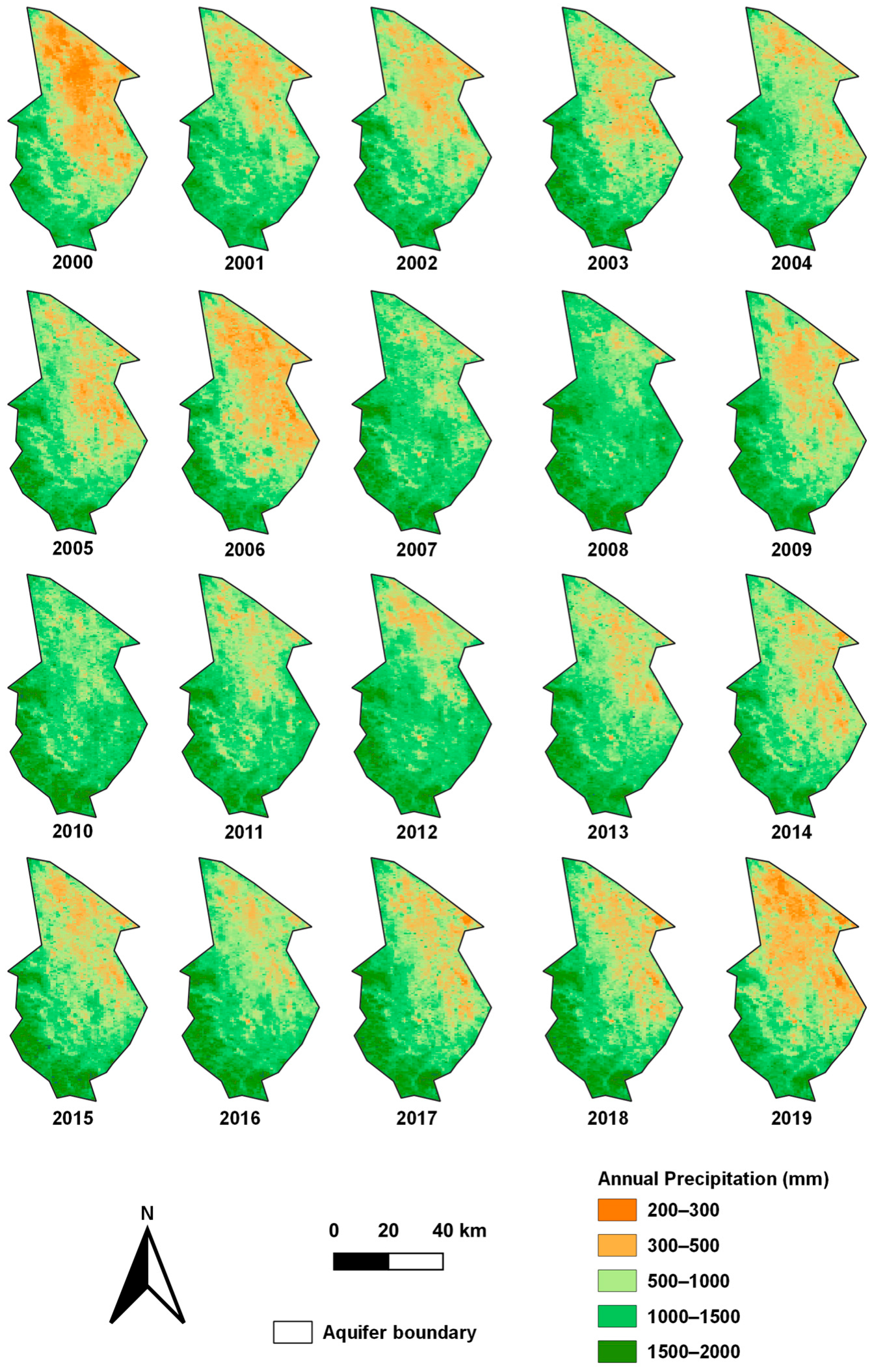
3.1. Spatiotemporal Variation in Precipitation

Figure 4 shows the estimated precipitation pattern in the study area, bounded by the limit of the aquifer, for the years 2000–2019 computed by using the temporal composite of maximum annual NDVI, built with daily remotely sensed data. When analyzing Figure 4, two temporal patterns can be seen. The first pattern can be considered from 2000 to 2006, while the second pattern can be seen from 2011 to 2019. The years 2007, 2008 and 2010 were wetter years, although 2009 was a drier year. In general, mostly the northern and middle regions of the study area, with a spatial pattern from northwest to east-central, have been mostly affected by water shortages, experiencing precipitation lower than 500 mm.

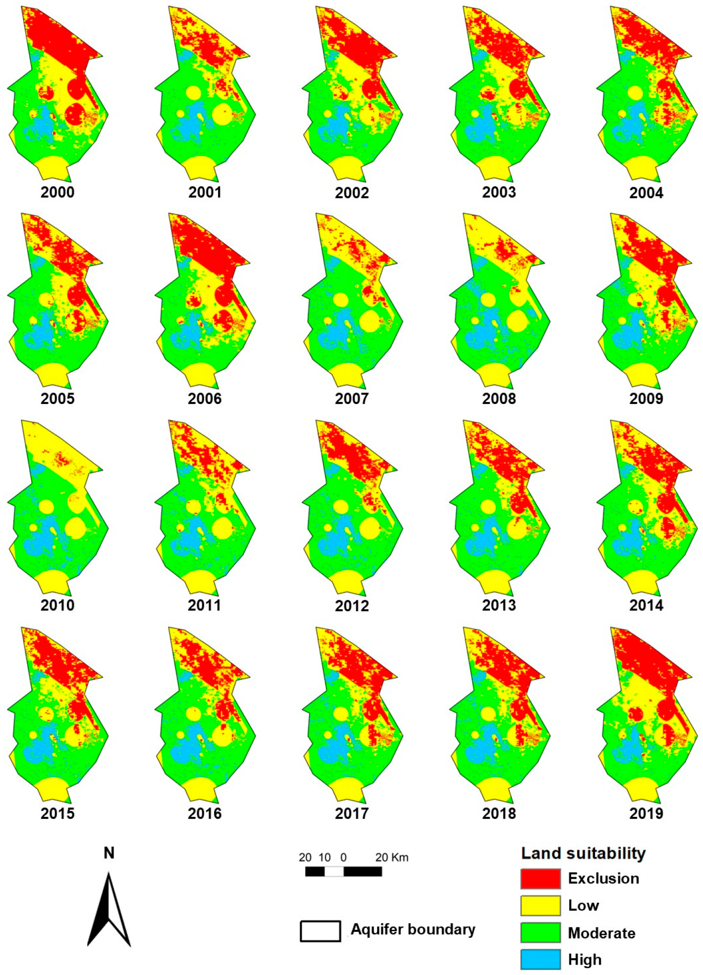
3.2. Spatial Pattern of Annual Land Suitability for Growing Orange Groves

Figure 5 reveals the spatiotemporal pattern of land suitability for growing orange groves in the Rioverde region for every year, with an emphasis on the annual variability in precipitation. This spatial pattern of land suitability is strongly influenced by annual rainfall. Two areas of high land suitability for growing orange groves can be identified. The first land portion is at the center-south portion of the study area and can be distinguished as the greatest area of high land suitability (in blue), while a small portion of land is also exhibited in the northwest part of the study area.

3.3. Principal Component Analysis

Table A3. Matrix of eigenvalues, eigenvectors, and variance explained obtained from the principal component analysis executed to integrate annual land suitability values into a homogenous PCA-based land suitability map, i.e., PC1 map.

PC’s	PC1	PC2	PC3	PC4	PC5	PC6	PC7	PC8	PC9	PC10	PC11	PC12	PC13	PC14	PC15	PC16	PC17	PC18	PC19	PC20
% Variance explained	99.62	0.09	0.04	0.03	0.03	0.02	0.02	0.02	0.02	0.02	0.01	0.01	0.01	0.01	0.01	0.01	0.01	0.01	0.00	0.00
Eigenvalue	19.92	0.02	0.01	0.01	0.01	0.00	0.00	0.00	0.00	0.00	0.00	0.00	0.00	0.00	0.00	0.00	0.00	0.00	0.00	0.00
Eigenvector 1 (Year 2000)	0.22	−0.21	−0.36	0.22	−0.59	0.56	−0.18	0.04	−0.03	0.13	−0.05	0.00	0.01	0.02	−0.01	−0.10	0.00	−0.03	−0.01	0.00
Eigenvector 2 (Year 2001)	0.22	0.15	0.11	−0.15	0.09	0.07	−0.07	0.12	−0.20	0.06	−0.17	0.01	−0.07	−0.20	0.52	−0.46	−0.47	0.18	0.01	0.00
Eigenvector 3 (Year 2002)	0.22	−0.17	−0.07	−0.29	0.06	0.11	0.33	0.26	−0.29	−0.11	−0.05	0.53	0.04	−0.43	−0.19	0.13	0.16	0.00	0.00	0.00
Eigenvector 4 (Year 2003)	0.22	−0.05	−0.04	−0.41	−0.09	0.00	0.04	0.56	0.08	−0.27	0.19	−0.35	−0.28	0.32	−0.10	0.11	−0.13	−0.02	0.00	0.00
Eigenvector 5 (Year 2004)	0.22	−0.12	0.05	−0.10	0.12	−0.12	−0.53	−0.16	−0.47	0.10	0.46	0.22	0.00	0.27	−0.11	−0.04	0.04	0.10	−0.02	0.00
Eigenvector 6 (Year 2005)	0.22	−0.05	−0.11	−0.31	−0.19	−0.29	−0.12	−0.12	0.66	0.17	0.27	0.16	0.08	−0.25	−0.02	−0.22	0.04	0.07	−0.01	0.00
Eigenvector 7 (Year 2006)	0.22	−0.30	−0.28	0.16	0.11	−0.25	−0.27	−0.23	0.00	−0.63	−0.23	−0.14	−0.12	−0.24	0.07	0.05	−0.01	−0.02	0.00	0.00
Eigenvector 8 (Year 2007)	0.22	0.30	−0.02	0.02	0.00	−0.11	−0.05	−0.04	−0.06	0.12	−0.05	0.07	−0.27	−0.04	−0.01	−0.06	0.00	−0.86	0.04	0.00
Eigenvector 9 (Year 2008)	0.22	0.42	−0.12	0.14	−0.06	−0.10	0.05	−0.05	0.00	0.03	−0.07	0.07	−0.25	0.02	−0.07	0.17	0.03	0.27	−0.74	0.00
Eigenvector 10 (Year 2009)	0.22	−0.17	0.06	−0.27	−0.11	−0.07	0.17	−0.29	0.09	0.00	−0.46	0.31	0.09	0.59	0.14	0.12	−0.08	−0.02	0.02	0.00
Eigenvector 11 (Year 2010)	0.22	0.41	−0.15	0.18	−0.08	−0.11	0.09	−0.07	−0.02	0.04	−0.02	0.08	−0.29	0.02	−0.12	0.14	0.01	0.35	0.67	0.00
Eigenvector 12 (Year 2011)	0.22	0.35	−0.12	0.07	0.05	0.09	0.23	−0.08	−0.03	−0.38	0.15	−0.05	0.57	0.18	−0.23	−0.39	−0.01	−0.06	−0.01	0.00
Eigenvector 13 (Year 2012)	0.22	0.23	−0.04	0.00	0.12	0.09	−0.26	0.19	0.10	0.05	0.02	−0.04	0.49	−0.08	0.38	0.60	0.03	−0.06	0.06	0.00
Eigenvector 14 (Year 2013)	0.22	−0.04	0.20	−0.07	0.19	0.08	−0.24	0.00	0.05	0.26	−0.39	−0.24	0.14	−0.15	−0.63	0.04	−0.29	0.05	0.01	0.00
Eigenvector 15 (Year 2014)	0.22	−0.11	0.06	−0.18	−0.27	−0.17	0.37	−0.38	−0.33	0.20	0.15	−0.51	0.10	−0.19	0.10	0.15	0.04	0.00	−0.01	0.00
Eigenvector 16 (Year 2015)	0.22	−0.08	0.20	0.02	0.39	0.58	0.16	−0.36	0.26	−0.10	0.30	0.00	−0.27	−0.02	0.06	0.12	−0.08	−0.01	−0.01	0.00
Eigenvector 17 (Year 2016)	0.22	0.05	0.21	−0.09	0.13	0.11	−0.12	0.08	0.02	0.06	−0.25	−0.20	−0.06	0.03	0.12	−0.27	0.79	0.09	0.03	0.00
Eigenvector 18 (Year 2017)	0.22	−0.15	0.43	0.37	−0.16	−0.15	0.08	0.17	0.06	−0.06	0.07	0.08	0.03	0.00	0.02	0.00	−0.04	−0.01	0.00	−0.71
Eigenvector 19 (Year 2018)	0.22	−0.15	0.43	0.37	−0.16	−0.15	0.08	0.17	0.06	−0.06	0.07	0.08	0.03	0.00	0.02	0.00	−0.04	−0.01	−0.01	0.71
Eigenvector 20 (Year 2019)	0.22	−0.31	−0.45	0.31	0.46	−0.17	0.26	0.20	0.04	0.40	0.04	−0.08	0.03	0.17	0.07	−0.10	0.00	0.00	−0.02	0.00

in Appendix A presents the coefficients obtained for each principal component based on annual land suitability for growing orange groves in the Rioverde region. The first principal component captured 99.62% of the variance associated with the spatial distribution of land suitability of orange groves regarding the spatiotemporal behavior of annual precipitation in the study area; that is, the first component efficiently incorporated the spatial and temporal distribution of every annual land suitability map computed using the NDVI-based annual precipitation. Indeed, the coefficients and loadings calculated for the first principal component were the same for all the years (0.22 and 0.99, respectively) (Appendix A, Table A3 and

Table A4. Matrix of loadings for principal components.

	PC1	PC2	PC3	PC4	PC5	PC6	PC7	PC8	PC9	PC10
Loading Year 2000	0.9972	−0.0283	−0.0313	0.0160	−0.0422	0.0394	−0.0114	0.0025	−0.0018	0.0075
Loading Year 2001	0.9986	0.0207	0.0095	−0.0110	0.0065	0.0049	−0.0042	0.0075	−0.0116	0.0035
Loading Year 2002	0.9982	−0.0231	−0.0061	−0.0208	0.0046	0.0077	0.0209	0.0156	−0.0170	−0.0059
Loading Year 2003	0.9983	−0.0066	−0.0039	−0.0296	−0.0062	0.0000	0.0028	0.0337	0.0048	−0.0152
Loading Year 2004	0.9983	−0.0164	0.0045	−0.0071	0.0084	−0.0084	−0.0337	−0.0095	−0.0274	0.0055
Loading Year 2005	0.9982	−0.0070	−0.0094	−0.0227	−0.0134	−0.0207	−0.0077	−0.0070	0.0385	0.0095
Loading Year 2006	0.9975	−0.0417	−0.0243	0.0114	0.0077	−0.0174	−0.0169	−0.0140	0.0000	−0.0353
Loading Year 2007	0.9985	0.0411	−0.0019	0.0016	−0.0002	−0.0075	−0.0032	−0.0026	−0.0034	0.0068
Loading Year 2008	0.9978	0.0573	−0.0103	0.0102	−0.0046	−0.0068	0.0029	−0.0028	−0.0002	0.0019
Loading Year 2009	0.9983	−0.0239	0.0052	−0.0195	−0.0076	−0.0052	0.0106	−0.0178	0.0054	0.0003
Loading Year 2010	0.9977	0.0567	−0.0129	0.0130	−0.0055	−0.0079	0.0056	−0.0044	−0.0009	0.0021
Loading Year 2011	0.9976	0.0480	−0.0104	0.0052	0.0039	0.0063	0.0145	−0.0051	−0.0018	−0.0214
Loading Year 2012	0.9983	0.0316	−0.0037	−0.0003	0.0083	0.0065	−0.0165	0.0112	0.0060	0.0027
Loading Year 2013	0.9986	−0.0061	0.0175	−0.0050	0.0132	0.0057	−0.0151	−0.0001	0.0032	0.0143
Loading Year 2014	0.9982	−0.0155	0.0056	−0.0132	−0.0189	−0.0122	0.0235	−0.0228	−0.0195	0.0109
Loading Year 2015	0.9979	−0.0109	0.0174	0.0014	0.0275	0.0405	0.0101	−0.0220	0.0155	−0.0054
Loading Year 2016	0.9988	0.0067	0.0186	−0.0067	0.0090	0.0078	−0.0078	0.0051	0.0011	0.0033
Loading Year 2017	0.9985	−0.0202	0.0375	0.0272	−0.0115	−0.0102	0.0048	0.0101	0.0035	−0.0035
Loading Year 2018	0.9985	−0.0202	0.0375	0.0273	−0.0115	−0.0103	0.0048	0.0101	0.0035	−0.0035
Loading Year 2019	0.9970	−0.0424	−0.0391	0.0228	0.0326	−0.0122	0.0163	0.0123	0.0024	0.0220
	PC11	PC12	PC13	PC14	PC15	PC16	PC17	PC18	PC19	PC20
Loading Year 2000	−0.0025	−0.0001	0.0004	0.0008	−0.0005	−0.0046	0.0001	−0.0011	−0.0002	0.0000
Loading Year 2001	−0.0092	0.0006	−0.0035	−0.0103	0.0253	−0.0221	−0.0213	0.0067	0.0002	0.0000
Loading Year 2002	−0.0025	0.0286	0.0023	−0.0223	−0.0090	0.0061	0.0072	0.0001	−0.0001	0.0000
Loading Year 2003	0.0105	−0.0191	−0.0151	0.0165	−0.0047	0.0051	−0.0057	−0.0006	0.0001	0.0000
Loading Year 2004	0.0251	0.0120	0.0002	0.0138	−0.0054	−0.0017	0.0017	0.0035	−0.0005	0.0000
Loading Year 2005	0.0150	0.0088	0.0044	−0.0131	−0.0009	−0.0103	0.0016	0.0024	−0.0003	0.0000
Loading Year 2006	−0.0128	−0.0076	−0.0065	−0.0123	0.0036	0.0024	−0.0002	−0.0008	0.0001	0.0000
Loading Year 2007	−0.0025	0.0039	−0.0144	−0.0022	−0.0007	−0.0028	−0.0002	−0.0317	0.0011	0.0000
Loading Year 2008	−0.0040	0.0038	−0.0133	0.0009	−0.0035	0.0079	0.0013	0.0099	−0.0198	0.0000
Loading Year 2009	−0.0253	0.0167	0.0047	0.0304	0.0067	0.0058	−0.0037	−0.0006	0.0006	0.0000
Loading Year 2010	−0.0009	0.0044	−0.0158	0.0009	−0.0057	0.0066	0.0006	0.0129	0.0178	0.0000
Loading Year 2011	0.0083	−0.0029	0.0306	0.0092	−0.0113	−0.0185	−0.0004	−0.0021	−0.0002	0.0000
Loading Year 2012	0.0010	−0.0024	0.0263	−0.0041	0.0185	0.0284	0.0012	−0.0024	0.0016	0.0000
Loading Year 2013	−0.0216	−0.0129	0.0073	−0.0078	−0.0305	0.0021	−0.0129	0.0018	0.0003	0.0000
Loading Year 2014	0.0084	−0.0277	0.0052	−0.0100	0.0047	0.0073	0.0017	−0.0001	−0.0003	0.0000
Loading Year 2015	0.0165	0.0000	−0.0145	−0.0010	0.0028	0.0056	−0.0035	−0.0003	−0.0003	0.0000
Loading Year 2016	−0.0138	−0.0108	−0.0035	0.0017	0.0058	−0.0130	0.0358	0.0034	0.0007	0.0000
Loading Year 2017	0.0041	0.0044	0.0018	0.0002	0.0007	0.0002	−0.0016	−0.0004	0.0000	−0.0001
Loading Year 2018	0.0040	0.0044	0.0018	0.0002	0.0007	0.0002	−0.0016	−0.0003	−0.0002	0.0001
Loading Year 2019	0.0023	−0.0042	0.0018	0.0086	0.0032	−0.0048	−0.0001	−0.0002	−0.0006	0.0000

). This reveals that all years were successfully represented by the first principal component; therefore, it captured deep detail of all principal components in the first one.

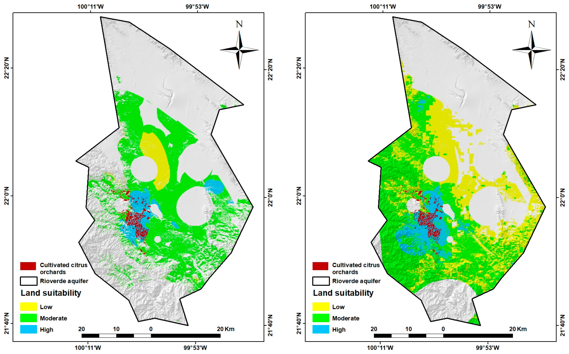
3.4. Integrated Land Suitability for Growing Orange Groves

Figure 6 shows the spatial distribution of orange groves in the Rioverde region based on MAP and PCA land suitability approaches. MAP-based land suitability reflects the spatial patterns of mean annual rainfall on land suitability, while PCA-based land suitability exhibits hidden spatial patterns of interannual variation in precipitation. Figure 7 presents a zoom-in of the main area for growing orange groves in the study area. According to the results shown in

Table 5. Estimated land suitability for orange groves in Rioverde, Mexico.

Land Suitability	MAP-Based Land Suitability		PCA-Based Land Suitability
	Area (ha)	Area (%)	Area (ha)	Area (%)
Exclusion	185,986.9	66.79	126,864.5	45.59
Low	7864.1	2.85	55,916.7	20.09
Moderate	74,168.8	26.67	79,845.7	28.69
High	10,246.9	3.69	15,639.8	5.62

, the total area of PCA-based high land suitability increased by 5392.9 ha with respect to the MAP-based high land suitability, i.e., an increase of 52.6% of the area with high land suitability.

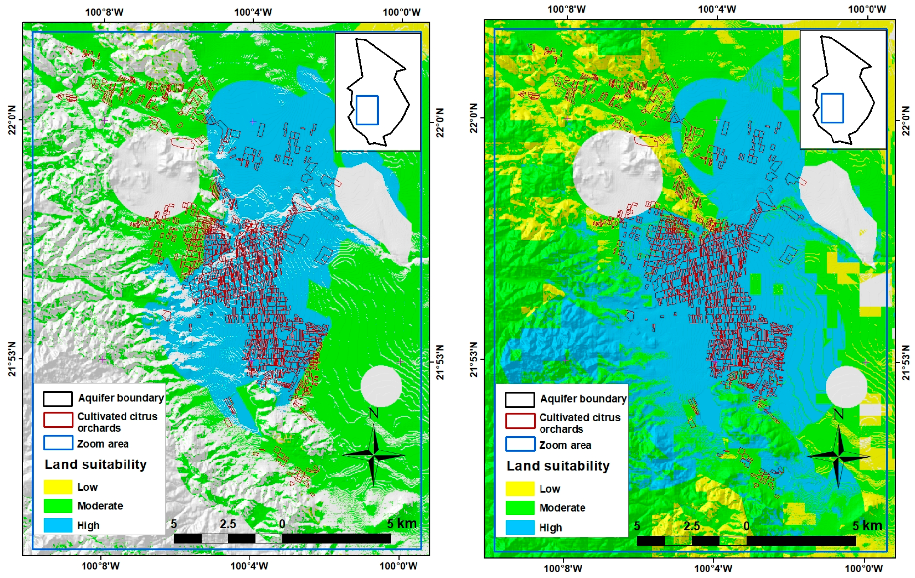
3.5. Comparison of Land Suitability Maps vs. Spatial Distribution of Orange Groves

Table 6. Areal comparison of current orange grove locations to estimated land suitability in Rioverde, Mexico.

Land Suitability	MAP-Based Land Suitability		PCA-Based Land Suitability
	Area (ha)	Area (%)	Area (ha)	Area (%)
Exclusion	547.47	19.26	44.1	1.55
Low	0.25	0.01	171.4	6.03
Moderate	550.46	19.37	493.7	17.37
High	1744.13	61.36	2133.1	75.05
Total	2842.3	100	2842.3	100

MAP: mean annual precipitation, PCA: principal component analysis.

presents the areal comparisons of MAP- and PCA-based land suitability estimates against the current orange grove map (ground truth). Regarding the MAP-based land suitability, 2294.6 ha, i.e., 80.73% of the total area of existing orange groves, were located in middle and high land suitability zones within the study area. Regarding PCA-based land suitability, it was discovered that 2626.8 ha, i.e., 92.42% of the total area of present orange groves, were located in middle and high land suitability zones within the study area.

4. Discussion

4.1. Spatiotemporal Variation in Precipitation

This study presented a methodology framework for modeling land suitability for growing orange groves in a portion of the citrus belt region in northern Mexico. Hypertemporal (daily) remote sensing data were highly effective in capturing the interannual variability in precipitation at the pixel level in the study area. Twenty-year NDVI time-series daily data were used to compute the maximum yearly NDVI and, therefore, annual precipitation. The spatiotemporal variation in precipitation was used to find the most suitable places for growing orange groves in terms of water availability. When observing the NDVI shown in Figure 4, the effect of precipitation on vegetation was revealed. Three great drought periods may be detected: 2000–2006; the sole year 2009; and 2011–2019.

Hypertemporal, i.e., time-series-based remote sensing, has been utilized for a variety of conditions or purposes. From worldwide studies to very local studies, hypertemporal remote sensing has remained a strategic tool for analyzing a variety of biophysical variables, including vegetation, i.e., flower bloom [76], impervious surfaces [77], land surface temperature [78], vegetation phenology [79], etc. Depending on the geographical extent, the spatial and temporal resolution may be compromised to find the best choice of hypertemporal analysis. Regarding the NDVI–rainfall relationship, some key studies have documented the relationship of the effect of rainfall on vegetation [80].

Few studies have been reported on the use of time-series remotely sensed data in Mexico. Although some studies have focused on land use change or phenology, the number of such studies is still limited. Miranda-Aragón et al. [35] conducted a study examining NDVI–rainfall trends over a larger area using 15-day remotely sensed data spanning a decade. Our study builds upon this work by utilizing Miranda-Aragón et al.’s exponential equation to estimate mean annual precipitation from daily temporal resolution time-series data ranging from 2000 to 2019. Upon comparing both studies’ remotely sensed data, a strong visual correlation during the first 11 years (2000–2010) is evident, with the dry years in their time series corresponding to the dry years in ours. Our study extends over a longer period, ranging from 2000 to 2020, and confirms that 2007, 2008, and 2010 were the wettest years of the period from 2000 to 2010, as found by Miranda-Aragón et al.’s work.

4.2. Spatial Pattern of Annual Land Suitability for Growing Orange Groves

This study utilized time-series remote sensing data to estimate annual precipitation, allowing us to evaluate the suitability of land for orange grove cultivation on an annual basis. This approach provided a spatiotemporal perspective of the Rioverde region and revealed the variation in land suitability over time. Notably, our results indicate that the northern portion of the study area is particularly sensitive to climate variation, particularly interannual rainfall variation. On the other hand, a noticeable condition in Figure 5 can also be perceived: the middle and southern parts of the study area show high stability of the spatial pattern of land suitability for orange groves. Both conditions demonstrate that the temporal pattern of land suitability in the Rioverde aquifer, our study area, exhibits strong variation; in specific areas, however, this pattern is relatively homogeneous over time.

Multi-criteria decision analyses are commonly employed to determine land suitability for crop cultivation, guided by several distinct rationales, including (1) the assessment of a single date or situation [81,82], (2) sensitivity analysis that considers some environmental criteria, e.g., freezing [24], soil salinity [83], and climate indexes [84], (3) consideration of planning scenarios devised by experts in relevant fields or stakeholders [85], (4) assessment of the impacts of climatic or land use potential scenarios [86], and (5) analysis of the effects of interannual NDVI on the variable of response, such as land suitability [18]. According to a study conducted in our research area, water availability, which is greatly influenced by climate variability, emerges as the most critical factor, after soil, affecting crop production [5]. Therefore, we investigated the impact of interannual rainfall variability on the determination of land suitability for orange groves, capturing land suitability variation for the period from 2000 to 2019 with an annual temporal resolution.

4.3. Integrated Land Suitability for Growing Orange Groves

Figure 6 depicts land suitability for growing orange groves in the Rioverde region. This study analyzed the spatial distribution of orange groves in the Rioverde region using both MAP and PCA land suitability approaches. The results showed that the PCA-based approach revealed hidden spatial patterns of interannual variation in precipitation, leading to a 52.6% increase in the total area with high land suitability compared with the MAP-based approach. PCA and MCDA are versatile approaches that have been used in a variety of situations and contexts. For example, Li and Yeh [87] used PCA to reduce the dimensionality of distance variables before running MCDA in a simulation of land use in Dongguan, Southern China. Carlón-Allende et al. [88] employed principal component analysis to identify the more dynamic variables in watershed hydrogeological regionalization in a study of watershed prioritization in Cuizeo Lake, and the final score for each watershed was obtained by using multi-criteria decision techniques. Seyedmohammadi et al. [19] applied multi-criteria decision techniques to determine the best location for growing maize, rapeseed, and soybean in northern Iran; the PCA technique was used to select important criteria for crop yield. All the aforementioned applications of both PCA and MCDA have been used separately or in a complementary way. In this research, PCA was used to assimilate the interannual variability effect of precipitation on annual land suitability. Therefore, the integration of the annual land suitability maps generated a more comprehensive and precise global map, indicating the advantages of using PCA in land suitability studies. This demonstrates the effectiveness of assimilating interannual variability effects using PCA, leading to improved accuracy and a better understanding of the spatial distribution of land suitable for growing oranges in the Rioverde region.

Studies have also highlighted the importance of analyzing land suitability and crop productivity, particularly in the context of climate change and water scarcity. For example, Jayathilaka et al. [89] conducted a study to determine land suitability for tea, rubber, and coconut crops in Sri Lanka using a multi-criteria decision analysis approach. The study analyzed data on rainfall, relative humidity, temperature, and evapotranspiration for two study periods: 1980–1992 and 1993–2007. The authors found that there was a decreasing trend in annual rainfall in the wet zone, which is located in the middle of the country. They also observed a significant increase of 1.4 °C in mean temperature across the entire country. These changing climatic conditions have led to a shift in the spatial patterns of crops throughout Sri Lanka. López-Blanco et al. [90] studied the land suitability for rainfed maize cultivation under climate change projections in Mexico at the national level. The authors concluded that a reduction in rainfall and an increase in temperature would have serious implications for national agriculture, particularly for rainfed maize. The study identified areas with high climate stability as well as regions that are more vulnerable to reduced maize yields in the future. By highlighting these zones, the study provides insight into the potential impacts of climate change on rainfed maize cultivation in Mexico.

4.4. Validation

Land suitability estimates obtained through MAP-based and PCA-based methods were compared against the spatial distribution of 2234 orange groves as ground truth. The results showed that both methods were effective in identifying areas with high and moderate suitability for orange groves, as the majority of existing orange groves were located in these zones. Specifically, 80.73% of existing orange groves were in the high and medium land suitability zones identified by the MAP-based method, while 92.42% of existing orange groves were located in the same zones according to the PCA-based method.

Figure 8 illustrates the Receiver Operating Characteristic (ROC) curves for two distinct land suitability assessment models: one based on mean annual precipitation (MAP) and the other employing principal component analysis (PCA). These curves effectively demonstrated each model’s capability in accurately distinguishing between areas with and without orange groves (AUC = 0.90 and 0.99, respectively). The ROC curves are instrumental in evaluating the overall efficacy of these land suitability models. In terms of interpreting the area under the curve (AUC) values derived from these ROC curves, they can be categorized as follows: AUC values ranging from 0.90 to 1.00 indicate ‘Excellent’ model performance, indicating a high level of accuracy in predictions. Values between 0.80 and 0.90 are indicative of ‘Good’ performance, reflecting competent but not flawless prediction capabilities. AUC values in the range of 0.70 to 0.80 are classified as ‘Fair,’ suggesting moderate predictive accuracy. ‘Poor’ model performance is associated with values between 0.60 and 0.70, where the models begin to show significant limitations. Finally, AUC values falling between 0.50 and 0.60 suggest that the model’s performance is no better than random chance, essentially lacking any discriminative ability.

In the context of MCDA, some researchers have validated their land suitability results in slightly different but interesting ways. Li et al. [16] validated their land suitability maps for tea crops in Zhejiang, China, using 3745 validation points obtained by global positioning system (GPS) receptors. After analyzing the tea crop locations located in highly and moderately suitable regions, the accuracy obtained was 87.91%. Dedeoğlu and Dengiz [18] employed a simple linear regression model to validate their analysis of wheat land suitability. They compared yield data as ground truth (response variable) against land suitability classes and NDVI to ensure accuracy. Remarkably, the study successfully validated the analysis by obtaining high determination coefficients of 0.83 (yield data vs. land suitability classes) and 0.78 (NDVI data vs. land suitability classes). Layomi-Jayasinghe et al. [91] validated their land suitability maps for tea crops by overlaying a spatial data layer of tea plantings with the predicted land suitability using MCDA. Their validation approach involved only considering agricultural fields that overlapped with very highly suitable and highly suitable areas. Impressively, this method resulted in an accuracy rate of 92.46%. Others have employed further validation approaches, such as the work of Tshabalala et al. [23] who used the so-called relative operating characteristic under the logistic regression framework. The authors evaluated land suitability for Moringa oleifera in South Africa and used logistic regression to estimate the area under the ROC curve, reporting an accuracy of 81%.

An additional perspective for validating our approach was to analyze the consistency ratio (CR < 0.1), which was obtained for both within-criteria and between-criteria pairwise comparison matrices. These matrices were used to calculate the weights in the context of MCDA. By examining the consistency ratio, we could measure any inconsistency in the judgment given by the expert and therefore gain further insight into the reliability of our approach. In this sense, all matrices had values lower than 0.1, that is, 0.03 for the criterion topography, 0.06 for the criterion soil, 0.07 for the criterion climate, 0.03 for the criterion proximity to water sources; finally, considering all four criteria, the consistency ratio was 0.01 [68]. Although consistency ratio measures do not guarantee the accuracy of our results, they can be used as an important signal of the robustness of our approach [71].

5. Conclusions

This study focused on exploring land suitability for establishing orange groves in a portion of the northern Mexican orange belt by combining variables related to topography, soil, climate, and proximity to water sources. Additionally, it utilized daily remote sensing data to infer historical annual precipitation patterns as part of a spatial variability analysis of land suitability or a form of land suitability sensitivity analysis based on the behavior of estimated annual precipitation using remote sensing data. The analysis was conducted from two perspectives: a) determining soil suitability using environmental variables while considering mean annual precipitation and b) considering precipitation as the integration of spatiotemporal patterns from daily remote sensing data collected over a 20-year period using principal component analysis. The first case resulted in a relatively homogeneous map of land suitability for establishing orange groves, whereas the second case initially revealed a larger area but with hidden patterns of land suitability for orange grove establishment.

Based on the analysis of land suitability classes, four conclusions can be drawn. For the class known as the exclusion class, the MAP-based approach depicts a vast majority of land as unsuitable (185,986.9 ha, 66.79% of the study area). This approach may overshadow the potential identified by a more integrative PCA approach (126,864.5 ha, 45.59%). The latter’s use of remotely sensed data likely captures a richer, more diverse environmental profile, suggesting that nearly half of the previously excluded land may have untapped agricultural potential. For the low-suitability class, low-suitability lands represent a small fraction when MAP-based land suitability is used (7864.1 ha, 2.85%). However, the PCA-based land suitability approach expands this category substantially, translating to a sevenfold increase in the identified area (55,916.7 ha, 20.09%). This indicates a considerable amount of land that, while not ideal, could be cultivated with appropriate agronomic management practices. For the moderate suitability class, the moderately suitable areas are comparable between the two methodologies (26.67% and 28.69%, respectively), with the PCA-based land suitability approach revealing slightly more land (79,845.7 ha). Based on remotely sensed data, these areas are likely to have favorable conditions but may still require enhancements in order to reach their full potential. For the high suitability class, high-suitability zones are critical for strategic cultivation due to their optimal conditions. The PCA-based land suitability approach indicates that a greater extent of land falls under this classification (15,639.8 ha, 5.62%) compared to the MAP-based land suitability approach (10,246.9 ha, 3.69%). This illustrates the importance of using sophisticated analytical tools to determine the best locations for cultivation.

The combination of these two methodologies offers valuable insights for agricultural planning and policy making. The MAP-based land suitability approach may be more conservative, potentially underestimating the land’s agricultural suitability. In contrast, the PCA-based land suitability approach, with its inclusion of remotely sensed data, provides a more expansive and potentially accurate assessment of land suitability. For effective agricultural development, it is crucial to leverage the PCA methodology’s comprehensive insights to identify areas where interventions can be most effective. This could involve enhancing water management in low-suitability areas or improving soil conditions in moderately suitable zones. The PCA-based land suitability approach also highlights the importance of remote sensing as a tool for agricultural assessment, offering a data-rich perspective that can guide precision agriculture practices. Overall, the study suggests that an integrative approach, combining precipitation data with remotely sensed information, can significantly improve the assessment of land suitability for orange crop cultivation. Such a methodological synergy could lead to informed decisions that promote sustainable agricultural expansion and optimization, ultimately leading to enhanced food security and economic development.

These research findings revealed the potential of principal component analysis of time-series remote sensing data to assimilate rainfall variation over time and then estimate a long-term land suitability map for growing orange groves. The modeling strategy exhibited new locations to grow citrus crops to tackle the problem of a reduction in the agricultural area due to urban growth in the Rioverde region (Mexico) as well as the effect of recurrent drought on water availability. Therefore, using more efficient irrigation systems, i.e., drop irrigation for producing specialty crops, will be the best option for optimizing water use. This methodology may be particularly relevant to those who need to make informed decisions about land use and water management strategies, especially in areas that are prone to climate variability and water scarcity. By integrating multiple criteria decision analysis, time-series remote sensing, and principal component analysis, this study offers a comprehensive approach to delineate the most suitable areas for sustainable citrus production in northern Mexico’s citrus belt. The results of this study may support decision-making processes for the effective land management of orange groves in the Rioverde region and provide valuable insights for managing agricultural production in other semiarid regions. Finally, this study demonstrates that the integration of MCDA and PCA could effectively identify areas that have been suitable for growing orange groves.

References

1. USDA. Citrus Annual; United States Department of Agriculture: Washington, DC, USA, 2021; p. 14. [Google Scholar]
2. Lozano, E. Citrus Annual. Available online: https://bit.ly/476DJ9l (accessed on 19 December 2023).
3. Dalin, C.; Wada, Y.; Kastner, T.; Puma, M.J. Groundwater Depletion Embedded in International Food Trade. Nature 2017, 543, 700–704. [Google Scholar] [CrossRef] [PubMed]
4. Campos-Aranda, D.F. Comparison of the Standardized Palmer Drought Index (SPDI) in Three Climatic Locations in San Luis Potosi, Mexico. Tecnol. Cienc. Agua. 2018, 9, 246–279. [Google Scholar] [CrossRef]
5. Charcas-Salazar, H.; Olivares-Sáenz, E.; Aguirre-Rivera, J.A. Irrigation water in Rioverde region, San Luis Potosi, Mexico. Ing. Hidraul. Mex. 2002, 17, 37–56. [Google Scholar]
6. Comisión Nacional del Agua (CONAGUA) Normales Climatológicas por Estado (1951–2010): San Luis Potosí. Available online: https://smn.conagua.gob.mx/es/informacion-climatologica-por-estado?estado=slp (accessed on 24 March 2020).
7. Chávez, L. Drought Conditions in Mexico and Its Effect on Agriculture; United States Department of Agriculture, Foreing Agricultural Service, Global Agricultural Information Network: Washington, DC, USA, 2021; p. 11. [Google Scholar]
8. Dobler-Morales, C.; Bocco, G. Social and Environmental Dimensions of Drought in Mexico: An Integrative Review. Int. J. Disaster Risk Reduct. 2021, 55, 102067. [Google Scholar] [CrossRef]
9. USDA. Citrus: World Markets and Trade; United States Department of Agriculture, Foreign Agricultural Service, World Agricultural Outlook Board/USDA: Washington, DC, USA, 2023. [Google Scholar]
10. Hernández-Morales, L.M.; García-Pérez, E.; Cortés-Flores, J.I.; Villegas-Monter, A.; Mora-Aguilera, J.A. Integral fertilization in Maarrs orange trees under production with Citrus Tristeza Virus (CTV) and HuangLongBing symptoms. Rev. Fitotec. Mex. 2021, 44, 59–66. [Google Scholar]
11. Van Vliet, J.; Eitelberg, D.A.; Verburg, P.H. A Global Analysis of Land Take in Cropland Areas and Production Displacement from Urbanization. Glob. Environ. Chang. 2017, 43, 107–115. [Google Scholar] [CrossRef]
12. Molina, E. Nutrición y Fertilización de la Naranja; International Plant Nutrition Institute (IPNI): San Carlos, Costa Rica, 2000; p. 8. [Google Scholar]
13. Shaloo; Bisht, H.; Jain, R.; Singh, R.P. Cropland Suitability Assessment Using Multi Criteria Evaluation Techniques and Geo-Spatial Technology: A Review. Indian J. Agri. Sci. 2022, 92, 554–562. [Google Scholar] [CrossRef]
14. Cicciù, B.; Schramm, F.; Schramm, V.B. Multi-Criteria Decision Making/Aid Methods for Assessing Agricultural Sustainability: A Literature Review. Environ. Sci. Policy 2022, 138, 85–96. [Google Scholar] [CrossRef]
15. Malczewski, J. GIS-Based Land-Use Suitability Analysis: A Critical Overview. Prog. Plan. 2004, 62, 3–65. [Google Scholar] [CrossRef]
16. Li, B.; Zhang, F.; Zhang, L.W.; Huang, J.F.; Jin, Z.F.; Gupta, D.K. Comprehensive Suitability Evaluation of Tea Crops Using GIS and a Modified Land Ecological Suitability Evaluation Model. Pedosphere 2012, 22, 122–130. [Google Scholar] [CrossRef]
17. Flynn, K.C. Site Suitability Analysis for Tef (Eragrostis Tef) within the Contiguous United States. Comput. Electron. Agric. 2019, 159, 119–128. [Google Scholar] [CrossRef]
18. Dedeoğlu, M.; Dengiz, O. Generating of Land Suitability Index for Wheat with Hybrid System Aproach Using AHP and GIS. Comput. Electron. Agric. 2019, 167, 105062. [Google Scholar] [CrossRef]
19. Seyedmohammadi, J.; Sarmadian, F.; Jafarzadeh, A.A.; McDowell, R.W. Development of a Model Using Matter Element, AHP and GIS Techniques to Assess the Suitability of Land for Agriculture. Geoderma 2019, 352, 80–95. [Google Scholar] [CrossRef]
20. Amini, S.; Rohani, A.; Aghkhani, M.H.; Abbaspour-Fard, M.H.; Asgharipour, M.R. Assessment of Land Suitability and Agricultural Production Sustainability Using a Combined Approach (Fuzzy-AHP-GIS): A Case Study of Mazandaran Province, Iran. Inf. Process. Agric. 2020, 7, 384–402. [Google Scholar] [CrossRef]
21. Pilevar, A.R.; Matinfar, H.R.; Sohrabi, A.; Sarmadian, F. Integrated Fuzzy, AHP and GIS Techniques for Land Suitability Assessment in Semi-Arid Regions for Wheat and Maize Farming. Ecol. Indic. 2020, 110, 105887. [Google Scholar] [CrossRef]
22. Tashayo, B.; Honarbakhsh, A.; Akbari, M.; Eftekhari, M. Land Suitability Assessment for Maize Farming Using a GIS-AHP Method for a Semi- Arid Region, Iran. J. Saudi Soc. Agric. Sci. 2020, 19, 332–338. [Google Scholar] [CrossRef]
23. Tshabalala, T.; Ncube, B.; Moyo, H.P.; Abdel-Rahman, E.M.; Mutanga, O.; Ndhlala, A.R. Predicting the Spatial Suitability Distribution of Moringa oleifera Cultivation Using Analytical Hierarchical Process Modelling. S. Afr. J. Bot. 2020, 129, 161–168. [Google Scholar] [CrossRef]
24. Elsheikh, R.; Mohamed Shariff, A.R.B.; Amiri, F.; Ahmad, N.B.; Balasundram, S.K.; Soom, M.A.M. Agriculture Land Suitability Evaluator (ALSE): A Decision and Planning Support Tool for Tropical and Subtropical Crops. Comput. Electron. Agric. 2013, 93, 98–110. [Google Scholar] [CrossRef]
25. Zabihi, H.; Ahmad, A.; Vogeler, I.; Said, M.N.; Golmohammadi, M.; Golein, B.; Nilashi, M. Land Suitability Procedure for Sustainable Citrus Planning Using the Application of the Analytical Network Process Approach and GIS. Comput. Electron. Agric. 2015, 117, 114–126. [Google Scholar] [CrossRef]
26. Mokarram, M.; Mirsoleimani, A. Using Fuzzy-AHP and Order Weight Average (OWA) Methods for Land Suitability Determination for Citrus Cultivation in ArcGIS (Case Study: Fars Province, Iran). Phys. A 2018, 508, 506–518. [Google Scholar] [CrossRef]
27. Tercan, E.; Dereli, M.A. Development of a Land Suitability Model for Citrus Cultivation Using GIS and Multi-Criteria Assessment Techniques in Antalya Province of Turkey. Ecol. Indic. 2020, 117, 106549. [Google Scholar] [CrossRef]
28. Orhan, O. Land Suitability Determination for Citrus Cultivation Using a GIS-Based Multi-Criteria Analysis in Mersin, Turkey. Comput. Electron. Agric. 2021, 190, 106433. [Google Scholar] [CrossRef]
29. Jolliffe, I.T. Principal Component Analysis, 2nd ed.; Springer Series in Statistics; Springer: New York, NY, USA, 2002; ISBN 978-0-387-95442-4. [Google Scholar]
30. Millward, A.A.; Piwowar, J.M.; Howarth, P.J. Time-Series Analysis of Medium-Resolution, Multisensor Satellite Data for Identifying Landscape Change. Photogramm. Eng. Remote Sens. 2006, 72, 653–663. [Google Scholar] [CrossRef]
31. Aguirre-Salado, C.A.; Treviño-Garza, E.J.; Aguirre-Calderón, O.A.; Jiménez-Pérez, J.; González-Tagle, M.A.; Miranda-Aragón, L.; Valdez-Lazalde, J.R.; Aguirre-Salado, A.I.; Sánchez-Díaz, G. Forest Cover Mapping in North-Central Mexico: A Comparison of Digital Image Processing Methods. GIScience Remote Sens. 2012, 49, 895–914. [Google Scholar] [CrossRef]
32. Corner, B.R.; Narayanan, R.M.; Reichenbach, S.E. Noise Reduction in Remote Sensing Imagery Using Data Masking and Principal Component Analysis. In Proceedings of the Applications of Digital Image Processing XXIII, San Diego, CA, USA, 31 July–3 August 2000; Tescher, A.G., Ed.; Society of Photo-Optical Instrumentation Engineers: San Diego, CA, USA, 2000; pp. 1–11. [Google Scholar]
33. Mohan-Babu, M.Y.; Subramanyam, M.V.; Giri-Prasad, M.N. PCA Based Image Denoising. Signal Image Process. Int. J. 2012, 3, 236–244. [Google Scholar] [CrossRef]
34. Lasaponara, R. On the Use of Principal Component Analysis (PCA) for Evaluating Interannual Vegetation Anomalies from SPOT/VEGETATION NDVI Temporal Series. Ecol. Model. 2006, 194, 429–434. [Google Scholar] [CrossRef]
35. Miranda-Aragón, L.; Treviño-Garza, E.; Jiménez-Pérez, J.; Aguirre-Calderón, O.A.; González-Tagle, M.A.; Pompa-García, M.; Aguirre-Salado, C.A. NDVI-Rainfall Relationship Using Hyper-Temporal Satellite Data in a Portion of North Central Mexico (2000–2010). Afr. J. Agric. Res. 2012, 7, 1023–1033. [Google Scholar] [CrossRef]
36. Colditz, R.R.; Cord, A.; Conrad, C.; Mora, F.; Maeda, P.; Ressl, R. Analyzing Phenological Characteristics of Mexico with MODIS Time Series Products. In Proceedings of the MultiTemp2009, Mystic, CT, USA, 28 July 2009. [Google Scholar]
37. Colditz, R.R.; Llamas, R.M.; Ressl, R.A. Detecting Change Areas in Mexico Between 2005 and 2010 Using 250 m MODIS Images. IEEE J. Sel. Top. Appl. Earth Obs. Remote Sens. 2014, 7, 3358–3372. [Google Scholar] [CrossRef]
38. Colditz, R.R.; Ressl, R.A.; Bonilla-Moheno, M. Trends in 15-Year MODIS NDVI Time Series for Mexico. In Proceedings of the 2015 8th International Workshop on the Analysis of Multitemporal Remote Sensing Images (Multi-Temp), Annecy, France, 22–24 July 2015; IEEE: Piscataway, NJ, USA, 2015; pp. 1–4. [Google Scholar]
39. Rosegrant, M.W.; Ringler, C.; Zhu, T. Water for Agriculture: Maintaining Food Security under Growing Scarcity. Annu. Rev. Environ. Resour. 2009, 34, 205–222. [Google Scholar] [CrossRef]
40. Majsztrik, J.C.; Behe, B.; Hall, C.R.; Ingram, D.L.; Lamm, A.J.; Warner, L.A.; White, S.A. Social and Economic Aspects of Water Use in Specialty Crop Production in the USA: A Review. Water 2019, 11, 2337. [Google Scholar] [CrossRef]
41. Jurišić, M.; Radočaj, D.; Šiljeg, A.; Antonić, O.; Živić, T. Current Status and Perspective of Remote Sensing Application in Crop Management. J. Cent. Eur. Agric. 2021, 22, 156–166. [Google Scholar] [CrossRef]
42. Svoboda, M.D.; Fuchs, B.A. Handbook of Drought Indicators and Indices; World Meteorological Organization: Geneva, Switzerland, 2016; ISBN 978-92-63-11173-9. [Google Scholar]
43. DOF Agreement Disclosing the Technical Studies of National Groundwater of the Río Verde Aquifer, Code 2415, in the State of San Luis Potosí, Northern Gulf Administrative Hydrological Region—In Spanish: Acuerdo por el que se dan a Conocer los Estudios Técnicos de Aguas Nacionales Subterráneas del Acuífero Río Verde, Code 2415, en el Estado de San Luis Potosí, Región Hidrológico Administrativa Golfo Norte. Available online: https://bit.ly/3FfBaXc (accessed on 10 March 2023).
44. Comisión Nacional del Agua (CONAGUA) Actualización de la Disponibilidad Media Anual de Agua en el Acuífero Rio Verde (2415), Estado de San Luis Potosí. Available online: https://bit.ly/3ZUm3dS (accessed on 10 March 2023).
45. Comisión Nacional del Agua (CONAGUA) Actualización de la Disponibilidad Media Anual de Agua en el Acuífero Rio Verde (2415), Estado de San Luis Potosí. Available online: https://bit.ly/3mLruh2 (accessed on 10 March 2023).
46. Instituto Nacional de Estadística y Geografía (INEGI) Continuo de Elevaciones Mexicano (CEM) Version 3.0. Aguascalientes, Aguascalientes, México. Available online: https://www.inegi.org.mx/app/geo2/elevacionesmex/ (accessed on 11 October 2021).
47. Yáñez-Rodríguez, M.A. Caracterización del Acuífero Río Verde, San Luis Potosí con el Método Magnetotelúrico. Master’s Thesis, Instituto Potosino de Investigación Científica y Tecnológica, San Luis Potosí, Mexico, 2019. [Google Scholar]
48. Díaz-Rivera, J.C. Análisis de la Dinámica Espacio-Temporal y Distribución Potencial de los Manantiales en el Valle de Rioverde, San Luis Potosí. Master’s Thesis, Universidad Autónoma de San Luis Potosí, San Luis Potosí, Mexico, 2018. [Google Scholar]
49. Instituto Nacional de Estadística y Geografía (INEGI) Conjunto de Datos Vectorial Edafológico, Serie II, Escala 1:250,000, Continuo Nacional San Luis Potosí. Aguascalientes, Aguascalientes, México. Available online: https://www.inegi.org.mx/app/biblioteca/ficha.html?upc=702825235673 (accessed on 25 June 2022).
50. Instituto Nacional de Estadística y Geografía (INEGI) Conjunto de Datos Vectorial Edafológico, Serie II, Escala 1:250,000, Continuo Nacional Ciudad Mante. Aguascalientes, Aguascalientes, México. Available online: https://www.inegi.org.mx/app/biblioteca/ficha.html?upc=702825235680 (accessed on 25 June 2022).
51. Instituto Nacional de Estadística y Geografía (INEGI) Conjunto de Datos Vectorial Edafológico, Serie II, Escala 1:250,000, Continuo Nacional Ciudad Valles. Aguascalientes, Aguascalientes, México. Available online: https://www.inegi.org.mx/app/biblioteca/ficha.html?upc=702825235710 (accessed on 25 June 2022).
52. Instituto Nacional de Estadística y Geografía (INEGI) Conjunto de Datos Vectorial Edafológico, Serie II, Escala 1:250,000, Continuo Nacional Guanajuato. Aguascalientes, Aguascalientes, México. Available online: https://www.inegi.org.mx/app/biblioteca/ficha.html?upc=702825235703 (accessed on 25 June 2022).
53. Instituto Nacional de Estadística y Geografía (INEGI) Conjunto de Datos de Perfiles de Suelos. Escala 1:250,000. Serie II (Continuo Nacional). Aguascalientes, Aguascalientes, México. Available online: https://www.inegi.org.mx/app/biblioteca/ficha.html?upc=702825266707 (accessed on 25 June 2022).
54. Sannidi, S.; Bindu, G.S.M.; Neelima, T.L.; Umadevi, M. Soil Quality Mapping in the Groundnut Belt of Erstwhile Mahabubnagar District, Telangana, India Using GIS. Curr. Sci. India 2022, 122, 600. [Google Scholar] [CrossRef]
55. New, M.; Lister, D.; Hulme, M.; Makin, I. A High-Resolution Data Set of Surface Climate over Global Land Areas. Clim. Res. 2002, 21, 1–25. [Google Scholar] [CrossRef]
56. Boz, A.O.; Donmez, Y.; Ozyavuz, M. Use of Climate Maps in Determining Sustainable Agriculture Areas. J. Environ. Prot. Ecol. 2020, 21, 1062–1071. [Google Scholar]
57. Wang, Z.; Schaaf, C.B.; Sun, Q.; Shuai, Y.; Román, M.O. Capturing Rapid Land Surface Dynamics with Collection V006 MODIS BRDF/NBAR/Albedo (MCD43) Products. Remote Sens. Environ. 2018, 207, 50–64. [Google Scholar] [CrossRef]
58. Rouse, R.W., Jr.; Haas, R.H.; Schell, J.A.; Deering, D.W. Monitoring Vegetation Systems in the Great Plains with ERTS; NASA’s Goddard Space Flight Center: Greenbelt, MD, USA, 1974; Volume 1, pp. 309–317. [Google Scholar]
59. Xu, Y.; Yang, Y.; Chen, X.; Liu, Y. Bibliometric Analysis of Global NDVI Research Trends from 1985 to 2021. Remote Sens. 2022, 14, 3967. [Google Scholar] [CrossRef]
60. Cheng, Y.; Zhang, L.; Zhang, Z.; Li, X.; Wang, H.; Xi, X. Spatiotemporal Variation and Influence Factors of Vegetation Cover in the Yellow River Basin (1982–2021) Based on GIMMS NDVI and MOD13A1. Water 2022, 14, 3274. [Google Scholar] [CrossRef]
61. Holben, B.N. Characteristics of Maximum-Value Composite Images from Temporal AVHRR Data. Int. J. Remote Sens. 1986, 7, 1417–1434. [Google Scholar] [CrossRef]
62. Instituto Nacional de Estadística y Geografía (INEGI) Mapas Topográficos. Escala 1:50,000. Serie III. San Luis Potosí. Aguascalientes, Aguascalientes, México. Available online: https://bit.ly/3JiGkTU (accessed on 15 April 2019).
63. QGIS Development Team QGIS Geographic Information System. 2021. Available online: https://qgis.org/en/site/ (accessed on 19 December 2023).
64. Ruiz-Corral, J.A.; Medina-García, G.; González-Acuña, I.J.; Flores-López, H.E.; Ramírez-Ojeda, G.; Ortíz Trejo, C.; Byerly Murphy, K.; Martínez-Parra, R.A. Requerimientos Agroecológicos de Cultivos, 2nd ed.; Instituto Nacional de Investigaciones Forestales, Agrícolas y Pecuarias (INIFAP): Tepatitlán de Morelos, Mexico, 2013; ISBN 978-607-37-0188-4. [Google Scholar]
65. Doorembos, J.; Kassam, A.H. Yield Response to Water; FAO Irrigation and Drainage Paper; Food and Agriculture Organization of the United Nations: Rome, Italy, 1979; p. 193. [Google Scholar]
66. Anderson, C.M. Manual Para Productores de Naranja y Mandarina de La Región Del Río Uruguay. Diversificación Productiva. Manual Serie “A” 2. Secretaría de Agricultura, Pesca y Alimentación, Instituto Nacional de Tecnología Agropecuaria (INTA). Estación Experimental Agropecuaria Concordia, Concordia, Entre Ríos, Argentina. Available online: https://bit.ly/4b5gr6M (accessed on 25 June 2022).
67. Steduto, P.; Hsiao, T.C.; Fereres, E.; Raes, D. Crop Yield Response to Water; Steduto, P., Ed.; FAO Irrigation and Drainage Paper; Food and Agriculture Organization of the United Nations: Rome, Italiy,, 2012; ISBN 978-92-5-107274-5. [Google Scholar]
68. Cengiz, T.; Akbulak, C. Application of Analytical Hierarchy Process and Geographic Information Systems in Land-Use Suitability Evaluation: A Case Study of Dümrek Village (Çanakkale, Turkey). Int. J. Sust. Dev. World. 2009, 16, 286–294. [Google Scholar] [CrossRef]
69. Saaty, T.L. Decision Making—The Analytic Hierarchy and Network Processes (AHP/ANP). J. Syst. Sci. Syst. Eng. 2004, 13, 1–35. [Google Scholar] [CrossRef]
70. Eastman, J.R. IDRISI Selva; Clark University: Worcester, MA, USA, 2012. [Google Scholar]
71. Rahman, R.; Saha, S.K. Remote Sensing, Spatial Multi Criteria Evaluation (SMCE) and Analytical Hierarchy Process (AHP) in Optimal Cropping Pattern Planning for a Flood Prone Area. J. Spat. Sci. 2008, 53, 161–177. [Google Scholar] [CrossRef]
72. Zolekar, R.B.; Bhagat, V.S. Multi-Criteria Land Suitability Analysis for Agriculture in Hilly Zone: Remote Sensing and GIS Approach. Comput. Electron. Agric. 2015, 118, 300–321. [Google Scholar] [CrossRef]
73. Díaz Monroy, L.G. Estadística Multivariada: Inferencia y Métodos, 2nd ed.; Colección Textos; Departamento de Estadística, Facultad de Ciencias, Universidad Nacional de Colombia: Bogotá, Colombia, 2007; ISBN 978-958-701-195-1. [Google Scholar]
74. CESAVESLP Datos de Distribución Espacial de las Huertas de Naranja en el Valle de Rioverde en San Luis Potosí (Mexico) 2022. Available online: http://www.cesaveslp.org.mx/ (accessed on 19 December 2023).
75. Aissaoui, M.; Maizi, D.; Benhamza, M.; Azzouz, K.; Belaroui, A.; Bengusmia, D. Identification and Mapping of Potential Recharge in the Middle Seybouse Sub-Catchment of the Guelma Region (North East of Algeria): Contribution of Remote Sensing, Multi-Criteria Analysis, ROC-Curve and GIS. AS-ITJGW 2023, 12, 25–37. [Google Scholar] [CrossRef]
76. Zang, Y.; Chen, X.; Chen, J.; Tian, Y.; Shi, Y.; Cao, X.; Cui, X. Remote Sensing Index for Mapping Canola Flowers Using MODIS Data. Remote Sens. 2020, 12, 3912. [Google Scholar] [CrossRef]
77. Xu, T.; Li, E.; Samat, A.; Li, Z.; Liu, W.; Zhang, L. Estimating Large-Scale Interannual Dynamic Impervious Surface Percentages Based on Regional Divisions. Remote Sens. 2022, 14, 3786. [Google Scholar] [CrossRef]
78. Xiong, Q.; Chen, W.; Luo, S.; He, L.; Li, H. Temporal and Spatial Variation of Land Surface Temperature in Recent 20 Years and Analysis of the Effect of Land Use in Jiangxi Province, China. Atmosphere 2022, 13, 1278. [Google Scholar] [CrossRef]
79. Wu, W.; Xin, Q. Characterizing Spring Phenological Changes of the Land Surface across the Conterminous United States from 2001 to 2021. Remote Sens. 2023, 15, 737. [Google Scholar] [CrossRef]
80. Herrmann, S.M.; Anyamba, A.S.; Tucker, C.J. Recent Trends in Vegetation Dynamics in the African Sahel and Their Relationship to Climate. Glob. Environ. Chang. 2005, 15, 394–404. [Google Scholar] [CrossRef]
81. Binte-Mostafiz, R.; Noguchi, R.; Ahamed, T. Agricultural Land Suitability Assessment Using Satellite Remote Sensing-Derived Soil-Vegetation Indices. Land 2021, 10, 223. [Google Scholar] [CrossRef]
82. Akhavan, S.; Jalalian, A.; Toomanian, N.; Honarjo, N. “Use of a GIS-Based Multicriteria Decision-Making Approach, to Increase Accuracy in Determining Soil Suitability”, Iran. Commun. Soil Sci. Plant Anal. 2023, 54, 690–705. [Google Scholar] [CrossRef]
83. Shafiezadeh, M.; Moradi, H.; Fakheran, S. Evaluating and Modeling the Spatiotemporal Pattern of Regional-Scale Salinized Land Expansion in Highly Sensitive Shoreline Landscape of Southeastern Iran. J. Arid Land 2018, 10, 946–958. [Google Scholar] [CrossRef]
84. Badr, G.; Hoogenboom, G.; Moyer, M.; Keller, M.; Rupp, R.; Davenport, J. Spatial Suitability Assessment for Vineyard Site Selection Based on Fuzzy Logic. Precis. Agric. 2018, 19, 1027–1048. [Google Scholar] [CrossRef]
85. Corral, S.; Legna-de la Nuez, D.; Romero-Manrique de Lara, D. Integrated Assessment of Biofuel Production in Arid Lands: Jatropha Cultivation on the Island of Fuerteventura. Renew. Sust. Ener. Rev. 2015, 52, 41–53. [Google Scholar] [CrossRef]
86. Zabihi, H.; Vogeler, I.; Amin, Z.M.; Gourabi, B.R. Mapping the Sensitivity of Citrus Crops to Freeze Stress Using a Geographical Information System in Ramsar, Iran. Weather Clim. Extrem. 2016, 14, 17–23. [Google Scholar] [CrossRef]
87. Li, X.; Yeh, A.G.O. Urban Simulation Using Principal Components Analysis and Cellular Automata for Land-Use Planning. Photogramm. Eng. Remote Sens. 2002, 68, 341–351. [Google Scholar]
88. Carlón-Allende, T.; Mendoza, M.E.; López-Granados, E.M.; Morales-Manilla, L.M. Hydrogeographical Regionalisation: An Approach for Evaluating the Effects of Land Cover Change in Watersheds. A Case Study in the Cuitzeo Lake Watershed, Central Mexico. Water Resour. Manag. 2009, 23, 2587–2603. [Google Scholar] [CrossRef]
89. Jayathilaka, P.M.S.; Soni, P.; Perret, S.R.; Jayasuriya, H.P.W.; Salokhe, V.M. Spatial Assessment of Climate Change Effects on Crop Suitability for Major Plantation Crops in Sri Lanka. Reg. Environ. Chang. 2012, 12, 55–68. [Google Scholar] [CrossRef]
90. López-Blanco, J.; Pérez-Damián, J.L.; Conde-Álvarez, A.C.; Gómez-Díaz, J.D.; Monterroso-Rivas, A.I. Land Suitability Levels for Rainfed Maize under Current Conditions and Climate Change Projections in Mexico. Outlook Agric. 2018, 47, 181–191. [Google Scholar] [CrossRef]
91. Layomi-Jayasinghe, J.; Kumar, L.; Sandamali, J. Assessment of Potential Land Suitability for Tea (Camellia sinensis (L.) O. Kuntze) in Sri Lanka Using a GIS-Based Multi-Criteria Approach. Agriculture 2019, 9, 148. [Google Scholar] [CrossRef]
Figure 1. Location map of the study area.
Agriengineering 06 00016 g001
Figure 2. Variables used in the analysis.
Agriengineering 06 00016 g002
Figure 3. Flowchart of the methodology used [35].
Agriengineering 06 00016 g003
Figure 4. Spatiotemporal distribution of remote sensing-based annual precipitation built with NDVI daily data in the study area.
Agriengineering 06 00016 g004
Figure 5. Land suitability for orange groves estimated by using remote-sensing-based annual precipitation for every year: 2000–2019.
Agriengineering 06 00016 g005
Figure 6. Land suitability estimated by mean annual precipitation (MAP-based land suitability); mean annual precipitation derived from interpolating meteorological station data (left). Land suitability determined by integrating 20 years of suitability data using principal component analysis (PCA-based land suitability) (right).
Agriengineering 06 00016 g006
Figure 7. Zoom-in to cultivated citrus orchards for validating estimated land suitability: MAP-based land suitability (left) and PCA-based land suitability (right).
Agriengineering 06 00016 g007
Figure 8. Area under the curve for MAP-based and PCA-based land suitability multi-criteria decision models.
Agriengineering 06 00016 g008