Autonomous Driving Strategy for a Specialized Four-Wheel Differential-Drive Agricultural Rover

Abstract

Recently, the agriconstruction machinery sector has been involved in a great technological revolution. The reasons that may explain this are strictly connected to the mitigation of climate change. At the same time, there is a necessity to ensure an adequate production level in order to meet the increasing food demand due to the current population growth trend. In this context, the development of autonomously driven agricultural vehicles is one of the areas on which tractor manufacturers and academics are focusing. The fundamental prerequisite for an autonomous driving vehicle is the development of an appropriate motion strategy. Hence, the vehicle will be able to follow predetermined routes, accomplishing its missions. The aim of this study was the development of path-planning and path-following algorithms for an agricultural four-whee differential-drive vehicle operating in vineyard/orchard environments. The algorithms were completely developed within the MATLAB software environment. After a brief description of the geometrical characteristics of the vehicle, a parametric process to build a virtual orchard environment is proposed. Then, the functional principles of the autonomous driving algorithms are shown. Finally, the algorithms are tested, varying their main tuning parameters, and an indicator to quantify the algorithms’ efficiency, named relative accuracy, is defined. The results obtained show the strong dependence between the relative accuracy and lookahead distance value assigned to the rover. Furthermore, an analysis of rover positioning errors was performed. The results in this case show a lower influence of the location error when the accuracy of the positioning device is within 2 cm.

1. Introduction

The agricultural sector plays a fundamental role in modern economics. According to the Food and Agriculture Organization of the United Nations (FAO), almost one-third of the worldwide population is involved in the primary sector, generating an income of USD 3.5 trillion globally [1]. The importance of this sector is expected to grow, since the worldwide population growth trend is quite remarkable: indeed, estimates indicate that the global population will reach almost 10 billion people by 2050 [2]. Thus, it will be necessary to ensure that the increasing food demand is met. Another important topic for the agricultural sector is represented by climate change [3,4]. There is a double relationship between climate change and agriculture. On the one hand, the agricultural sector is one of the main actors in terms of greenhouse gas emissions: indeed, agriculture is responsible for 11% of the overall anthropogenic GHG emissions [5] (with peaks of 35% for developing countries) [6,7,8,9]. On the other hand, the effects of climate change are causing extreme weather and unpredictable weather events, which may affect future crop production [10,11]. Last but not least, the decline in the general agri-worker population should also be taken into consideration [12].

For all of these reasons, the agricultural machinery industry is at the heart of an authentic industrial revolution. The aim of this revolution is to increase productivity [13], both in terms of quality and quantity, efficiently. In this sense, the innovation attempts conducted by the academic and the industrial world can be explained. They are trying to pursue sustainability and, at the same time, increase efficiency through studying alternative tractor powertrains [14,15,16] and propellants [17,18,19,20] and the design of automated platforms [21,22]. One of the outputs, which can provide all the aforementioned features, is agricultural robots [23,24].

Agricultural robots are smart and automated vehicles designed to execute different operations, from soil preparation to harvesting, spraying applications, and monitoring field health status [25,26]. The benefits linked with the diffusion of agricultural robots involve several areas: environment, politics, and society [27]. Indeed, autonomous agricultural vehicles can lead to the better management of the use of pesticides and water [27,28]. Agricultural rovers are often equipped with electric powertrains and are lighter than the traditional forms of machinery, reducing greenhouse gas emissions and, at the same time, soil compaction [29]. The practice of precision farming enabled by agricultural robots can help famers to improve their resource management, such as fertilizer use or harvesting time, thus increasing crop productivity and quality [29,30]. One key element of an autonomous agricultural robot is its autonomous driving algorithm, through which the vehicle can make decisions in terms of the best strategy that it must adopt in order to reach a predetermined goal point [31].

The pillars of an autonomous driving algorithm are the path-planning and path-following phases. Autonomous driving applications for agricultural robots have been relatively widely investigated in the literature. In the study presented by Han et al. [32] on the performance of autonomous sprayers in orchards, the path planning phase was conducted by manually driving the vehicle, which followed the planned route by regulating its right and left crawler speeds. Ko et al. [33] developed a testing platform for precision spraying applications. In this case, the planning strategy was based on tracking line recognition, whereas the path-following algorithm was based on image-detection criteria. Many works focused only on the path-planning phase [34]. Han et al. [35] proposed an optimized path-planning strategy for a fleet of multiple unmanned tractors in peach orchards in order to improve the operating time, whereas Hameed developed a path-planning algorithm to improve fuel consumption [36]. Furthermore, some studies have applied planning strategies that take into account the condition of the soil [37,38] or robot dynamics [39]. Other studies, meanwhile, have focused their attention on the path-following stage [40,41]. Huang et al. developed an optimization control method for the headland turning management of front-wheel-steering vehicles using a pure pursuit-based strategy [42]. Peng et al. proposed a strategy for a four-independent-wheel-drive agricultural vehicle based on a non-lookahead strategy [43].

In the existing literature, according to the authors’ knowledge, few papers have investigated the motion strategy of an autonomously driven agricultural rover in its entirety. Indeed, some of them have focused only on one of the key elements of an autonomous driving algorithm. Considering the agricultural rover sector, very few studies have dealt with the autonomous driving strategy for a four-wheel differential-drive rover. Furthermore, the range of the applicability of this study is one of its most interesting elements, since it provides a parametric motion planning strategy, and thus, it can be used for different types of crops and vehicles.

The aim of this work was to develop an autonomous driving algorithm for a four-wheel differential-drive agricultural robot operating in orchards/vineyards. The algorithm is based on a lookahead methodology and was completely developed within the MATLAB environment. After a brief description of the geometrical characteristics of the vehicle, a parametric process to build a virtual orchard environment is described. Then, the motion planning process and the path-following algorithm inspired from the pure pursuit controller are exposed. Finally, the results section shows the efficiency of the algorithm with respect to the main parameters, defining a performance indicator to quantify the effects of the parameters combination. The efficiency of the algorithm is guaranteed, also introducing a random location error. However, in this last case, the use of a threshold value on the minimum steering angle is recommended.

2. Materials and Methods

In this section, the developed autonomous driving algorithm is explained. The model was completely developed within the MATLAB (R2021b) software environment. Starting from the kinematic model adopted for the rover, the creation of a parametric operative virtual environment, for testing the algorithm, is shown. Then, the global path-planning and path-following algorithms are illustrated.

2.1. Vehicle Kinematic Model

First of all, before starting with the description of the autonomous driving algorithm developed in this study, it is appropriate to proceed with an outline of the geometrical and kinematic features of the rover. The vehicle considered in this article consists of a small-sized rover (Figure 1a). This kind of agricultural robot usually does not exceed 1.5 m in width and length [44], and it is used for monitoring operations such as disease and insect detection or plant health status tracking [45,46]. Considering the top view, the rover can be schematically represented as a rectangle of 1 × 1.5 m (width x wheelbase), equipped with a fixed-wheel drive (tire radius equal to 0.4 m) on every corner of the chassis. This means that each wheel speed can be controlled in an independent way with respect to the others. The fixed-wheel drive prevents modeling the steering behavior of the vehicle as a classic agricultural tractor, which is characterized by a front steering system and describable with a bicycle kinematic model. In this case, the vehicle must handle the speed of each wheel in order to turn corners. In this way, the rover satisfies the longitudinal and yaw speed requirements, emulating the functioning of a vehicle differential. The main advantage of this kind of vehicle is the possibility to consider its minimum turning radius equal to zero, whereas its disadvantage is primarily related to a higher lateral stress on the tires during turning. Furthermore, the rover is simpler from a mechanical point of view, due to the absence of a physical steering system.

The aim of this work is to demonstrate the reliability and the efficiency of the developed control logic. As a consequence, this study considers only the kinematic behavior of the agricultural robot. Given this premise, the following assumptions can be made:

• The vehicle consists of a rigid body; thus, all the effects related to its deformability can be ignored.
• The algorithm was developed considering a 2-D operative environment since the rover belongs to the category of land vehicles; hence, vertical movement is neglectable.
• The 2-D environment implies that the state of the vehicle is fully defined with three degrees of freedom: two translational (longitudinal and lateral movements), and one rotational (yaw) around the axis perpendicular to the movement plane.
• The 2-D environment also implies that the rolling and pitch angles can be ignored.
• The wheel–ground contact is in a condition of pure rolling.
• Lateral slip can be ignored because the rover working speed is quite low; thus, almost all the effects related to vehicle dynamics are neglectable.

The kinematic model, used in this work, aims to define the relationships among the operative conditions that the vehicle should satisfy (longitudinal and yaw speeds), and the operative parameters that allow the vehicle to achieve that specific condition (angular speeds of each wheel). Based on the hypothesis provided before, the rover object of study can be represented as a symmetrical two-wheel independent drive vehicle (Figure 1b).

The equations that rule the kinematic model adopted are the same described in [47]:

$${\mathsf{\omega }}_{\mathrm{r}}=\mathrm{v}·\frac{1}{\mathrm{r}}+\dot{\mathsf{\theta }}·\frac{\mathrm{l}}{\mathrm{r}}$$

(1)

$${\mathsf{\omega }}_{\mathrm{l}}=\mathrm{v}·\frac{1}{\mathrm{r}}-\dot{\mathsf{\theta }}· \frac{\mathrm{l}}{\mathrm{r}}$$

(2)

where:

• ${\mathsf{\omega }}_{\mathrm{r}}$ and ${\mathsf{\omega }}_{\mathrm{l}}$ are the angular velocities of the right and left wheels, respectively.
• v is the longitudinal speed of the vehicle.
• $\dot{\mathsf{\theta }}$ is the yaw speed of the vehicle.
• r is the wheel radius fixed at 0.2 m.
• l is the track width of the rover equal to 1 m.

2.2. Virtual Operative Environment Definition

Once the kinematic model is defined, it is necessary to build the virtual environment in which the rover must operate. As previously stated, the aim of this work is to provide an autonomous driving algorithm for a 4-wheel differential-drive vehicle operating in agricultural orchard cultivations. For this reason, the developed map consists of a bidimensional orchard field, characterized by a certain number of fruit plant rows equally distributed. Furthermore, a parametric map-building process was developed in order to enhance the field of application of this study. Indeed, it should be noted that orchard cultivations can vary a lot with respect to one another. As a consequence, the number and the dimensions of the fruit plant rows, as well the size of the fields, can be very different depending on the specific cultivation considered. The map, generated at the end of the building process, is substantially a matrix in which every element can have two different values:

• 1 in cases of the presence of an obstacle that the vehicle must avoid.
• 0 in cases of a free path.

The first step of the map generation process consists of the set-up of some parameters, shown in Figure 2a, as follows:

• The number of fruit plants in a row n.
• The width w and length l of each fruit plant row, expressed in meters.
• The width L1 and length L2 of the orchard field, expressed in meters.
• The dimensional value Ys to which each fruit plant row must start, expressed in meters.
• The value of mesh refinement m, defined as the number of matrix elements contained for each square meter.

The way through which the values are assigned can be explained with the following block diagram (Figure 2b).

Figure 2. (a) Setting the parameters of the map generation algorithm; (b) map generation parametrization process.

Figure 2. (a) Setting the parameters of the map generation algorithm; (b) map generation parametrization process.

Then, two other variables can be defined once the map parameters are determined:

• The number of free rows N, defined as:

  N = n +1

  (3)
• The recurring step of the fruit plant rows P, defined as:

  P = L1/N

  (4)
• The occupied row area A, defined as the product between w and l.

In this way, different configurations of orchards can be easily obtained (Figure 3).

In order to illustrate the path-planning and path-following algorithms of this work, the parameters considered for the map (Figure 4) were:

• n is equal to 9; hence, N is equal to 10.
• w is equal to 2 m, and l is equal to 80 m.
• L1 and L2 are equal to 100 m; hence, P is equal to 10.
• Y_s is equal to 10 m.

Figure 4. Map configuration for path following and path planning used in this study.

Figure 4. Map configuration for path following and path planning used in this study.

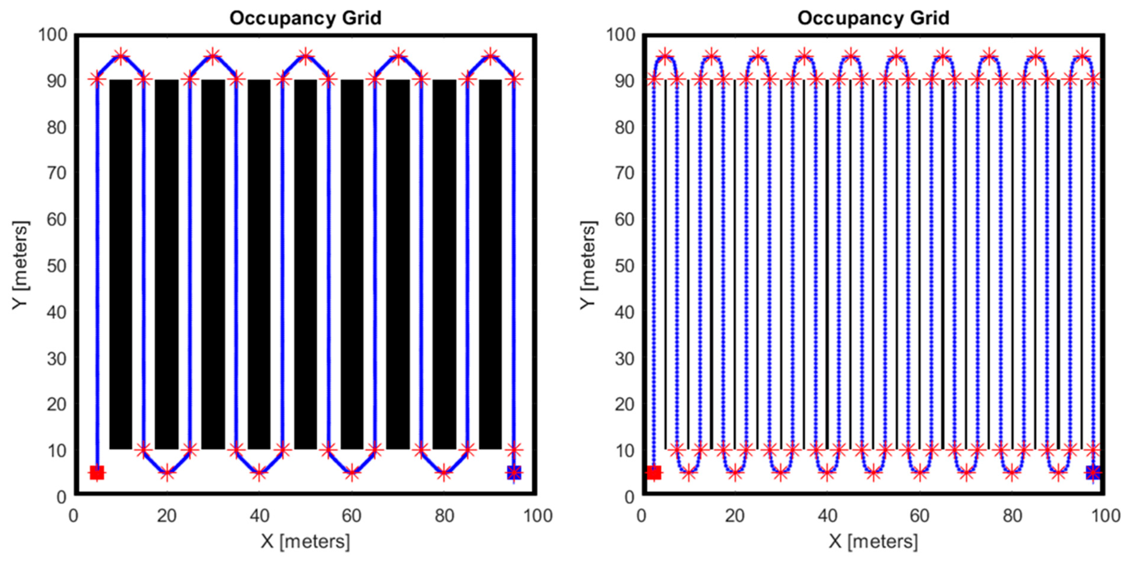
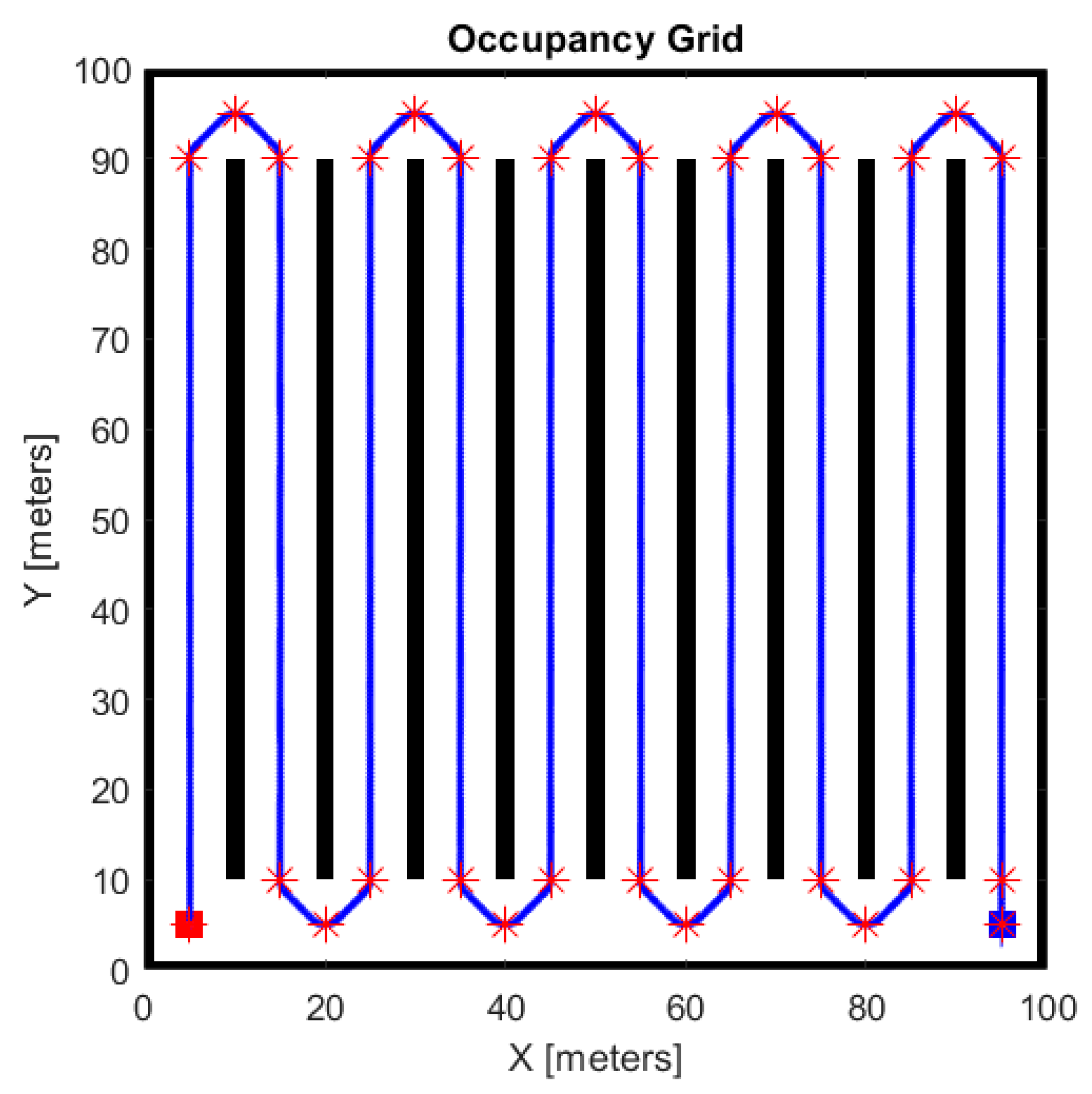
2.3. Global Path Planning

Once the virtual operative environment is built, the path that the vehicle must follow to accomplish its mission must be defined. This section of the autonomous driving algorithm is called global path planning since it considers the entire vehicle mission. The result of the motion planning process is the creation of a trajectory that allows for avoiding the known obstacles present on the map. On the contrary, the overcoming of unknown obstacles is not included. There are several methods for solving the motion planning problem, such as search-based or sample-based algorithms [48,49]. For this study, a path-planning algorithm based on Dubins path theory was used [50,51]. According to this methodology, the trajectory of an object can be traced with a combination of segments and circular arcs, given a start and an arrival point and their relative orientation on the map. This technique is particularly useful in the case of repetitive and structured operative environments, such as an orchard. In this way, the planned path can be obtained with a reduced computational cost. Indeed, in the case of an orchard, the vehicle usually executes two kinds of maneuvers:

• Traveling in a straight line along the fruit plant rows.
• Executing a hairpin turn in order to exit from a free row and enter the next one.

The motion planning problem has been solved parametrically even in this case. In this way the path that the vehicle must follow can be generated independently from the orchard considered. The adopted strategy consists of defining a series of checkpoints, and, through their interpolation, the desired trajectory can be obtained. First of all, the start and goal points are manually positioned, defining their relative coordinates and the vehicle orientation on the map. Then, 2 checkpoints are positioned at the beginning and end of each free row (see Figure 2a) in order to define the straight path that the vehicle has to travel. The hairpin turn is obtained defining a three-point arc, whose apex is located alternatively at the head or at the tail of each fruit plant row. The last phase of the path-planning process consists of the definition of the number of waypoints through which the checkpoints have to be interpolated. The number of interpolating points is arbitrarily defined, assuming a certain distance between two consecutive waypoints, namely the waypoint pitch (WPP). The results obtainable with different configurations of orchards are shown in Figure 5.

For the map configuration considered in this study (Figure 4), the results are shown in Figure 6.

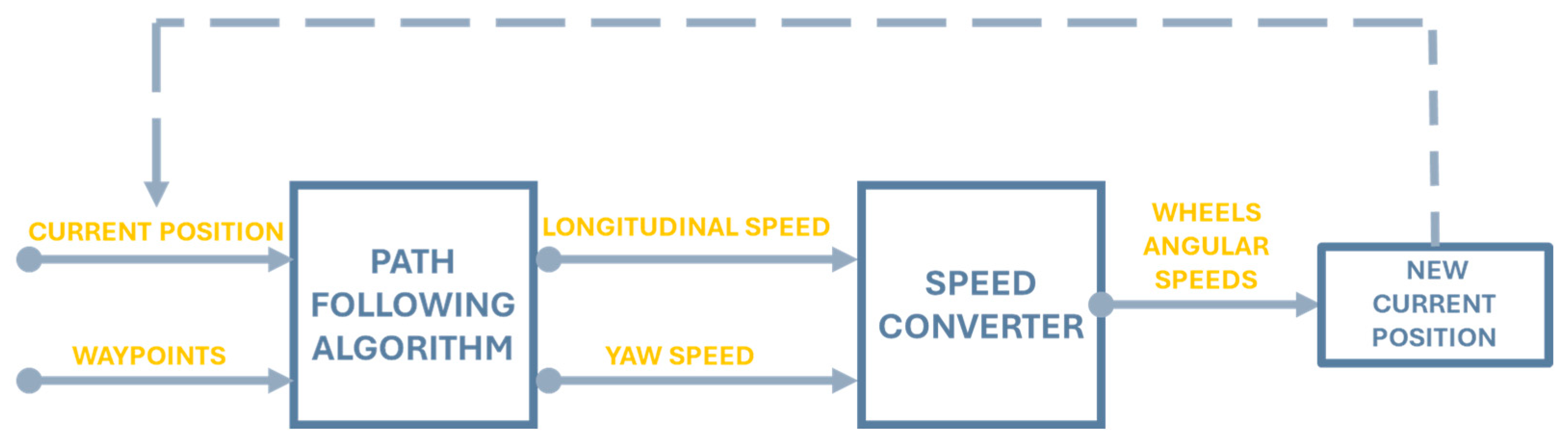
2.4. Path-Following Algorithm

The obtained waypoints represent the results of the path-planning process described in the previous subsection. They consist of a series of X-Y coordinates that the vehicle must follow to cover the predetermined path, grouped in a 2-D element vector. The output of the path-planning process represents the input of the path-following phase. The path-following control logic is structured as shown in Figure 7.

Given the waypoint and the current position of the rover, in each cycle, the path-following algorithm calculates the longitudinal and yaw speed necessary to reach the nearest waypoint. Then, both the speed terms are converted into the left and right wheel angular speed values, according to Equations (1) and (2). Lastly, the current position is updated, and the cycle repeats itself with the new current position input until the goal point is reached.

The path-following algorithm used in this work is inspired by the Pure Pursuit Controller [52,53]. According to this method, the aim is to identify the curvature that allows the vehicle to move from the start to the goal point. In this case, the scope is to determine the vehicle speed, intended as the longitudinal and yaw speeds, necessary for the path determined in the previous section. The algorithm is essentially made up of 2 phases:

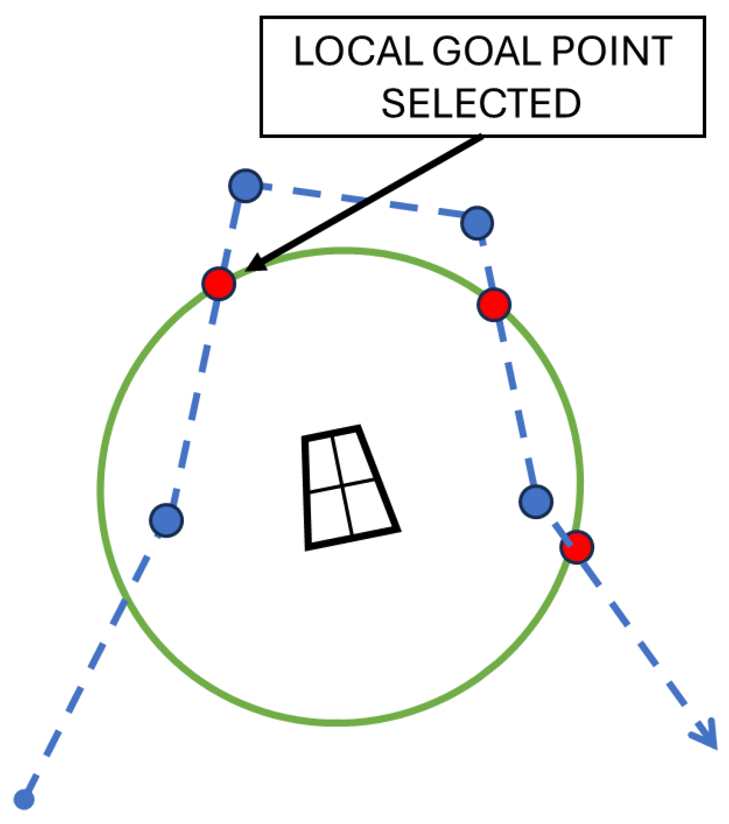
• Definition of a “local” goal point (LGP).
• Definition of the commands that must be imposed in a way that the rover can reach the goal point calculated in the previous step.

Concerning the first point, the algorithm identifies a local goal point at a certain distance from the actual rover position, called the lookahead distance (LD). To find the target point, the path-following strategy creates a circumference centered in the actual vehicle position, with a radius equal to LD (Figure 8).

The intersections between the circumference and the segments, which link the different waypoints, identify the potential local goal point. If more valid LGPs are defined, then the algorithm chooses the most appropriate one in order to follow the planned path. The way the control logic selects the most appropriate LGP is described in the next paragraphs. The LGP identification procedure repeats itself at each cycle until the final arrival point is reached. The correct definition of the lookahead distance plays a very important role for the successful execution of the rover mission. Indeed, if the LD value is too low, the vehicle may start to oscillate around the waypoints, whereas a high value of LD may trigger corner-cutting phenomena (Figure 9). Therefore, it is necessary to find the right balance to follow the planned path in the most efficient way.

Given two consecutive waypoints, P1 and P2, four situations can be generated by the interaction between the circumference and the straight line defined by P1 and P2:

• No intersections (Figure 10a).
• Single or multiple intersections with the straight line, but the points found are not included between P1 and P2 (Figure 10b); this case is interpreted by the algorithm as the previous one.
• Single intersection: The point found corresponds to the local goal point pursued by the rover (Figure 10c).
• Multiple intersections between P1 and P2: In this case, the algorithm chooses the nearest point to the second waypoint (Figure 10d).

Furthermore, two other measures must be adopted in order to make the algorithm more reliable. The first one is needed when the algorithm identifies several valid local goal points between more than two consecutive waypoints. This situation may occur when the rover drives tight or U-shaped corners (Figure 11).

In this situation, the vehicle selects as a local goal point the one identified in the segment defined by the first two waypoints. In this way, the rover avoids skipping a portion of the path by cutting the corner. A waypoint is marked as crossed when the distance between it and the rover center of mass is below a certain predefined threshold value D_th.

Lastly, a parameter called the current index has been defined and identifies the last valid waypoint crossed. In this way, the rover will not go back along the path because it considers local goal points associated with waypoints already passed as not valid. The current index is useful also in case no valid local goal point is detected by the rover; in this situation, the rover will move toward the last waypoint crossed and resume the pre-established path.

Once the local point has been identified, it is necessary to determine the longitudinal speed v and the yaw speed $\dot{\mathsf{\theta }}$, which are then used to calculate the angular speeds of the left and right wheels according to Equations (1) and (2). Considering the reference system defined in Figure 3, it is possible to define the angles, as shown in Figure 12:

• Vehicle direction γ defines the actual rover direction.
• Goal point angle φ defines the direction of the segment, which links the goal point and the rover center of mass, with respect to the reference system adopted and calculated using the atan2 function.
• Steering angle θ.

Figure 12. Graphical representation of the steering angle definition.

Figure 12. Graphical representation of the steering angle definition.

The steering angle θ is defined as:

θ = φ − γ

(5)

Given the steering angle and the cycle time t, the yaw speed can be defined as:

$$\dot{\mathsf{\theta }}=\mathsf{\theta }/\mathrm{t}$$

(6)

The longitudinal speed is defined as a function of the steering angle θ and calculable through the following equation:

v = v_t∙(1 − θ/θ_max)

(7)

where:

• v is the longitudinal speed of the vehicle.
• v_t is the maximum rover speed.
• θ is the steering angle.
• θ_max is the maximum steering angle and set to 360° because 4-wheel differential-drive vehicles ideally can execute a pivot maneuver.

The two speeds represent the output of the path-following algorithm, which is used to first calculate the wheel angular speeds and to update the current position of the vehicle.

The comprehensive flowchart of the autonomous driving algorithm developed for this work is reported in Figure 13.

3. Results and Discussion

In this section, the application of the autonomous driving algorithm for a four-wheel differential-drive vehicle is shown, focusing on its most important input parameters. However, before discussing the results analysis, it is very useful to recap the main features of the rover used in this study, which are displayed in

Table 1. Rover input parameters for path-following algorithm application.

Rover Features for Autonomous Driving Algorithm Application
Wheelbase	1.5 m
Track Width	1 m
Wheel Radius	0.2 m
Minimum Turning Radius	1 m
Reference Rover Speed	7 km/h

. They also represent the input variables on the basis of which the optimal trajectory was defined.

The value of 7 km/h was chosen as the reference rover speed because it represents an average value among the working speeds of agricultural vehicles, which range from 5 to 10 km/h [54].

Concerning the input parameters of the path-following algorithm, there are essentially two:

• Waypoint pitch (WPP): This indicates the distance (in meters) between two consecutive waypoints and can be obtained by splitting the total length of the planned path by the total number of waypoints.
• Lookahead distance (LD): This indicates the radius of the circumference that the vehicle uses to find the local goal point.

The correct planned trajectory pursuit by the rover can be obtained by adequately tuning these two variables.

For this study, two performance indicators were defined in order to evaluate the performance of the algorithm:

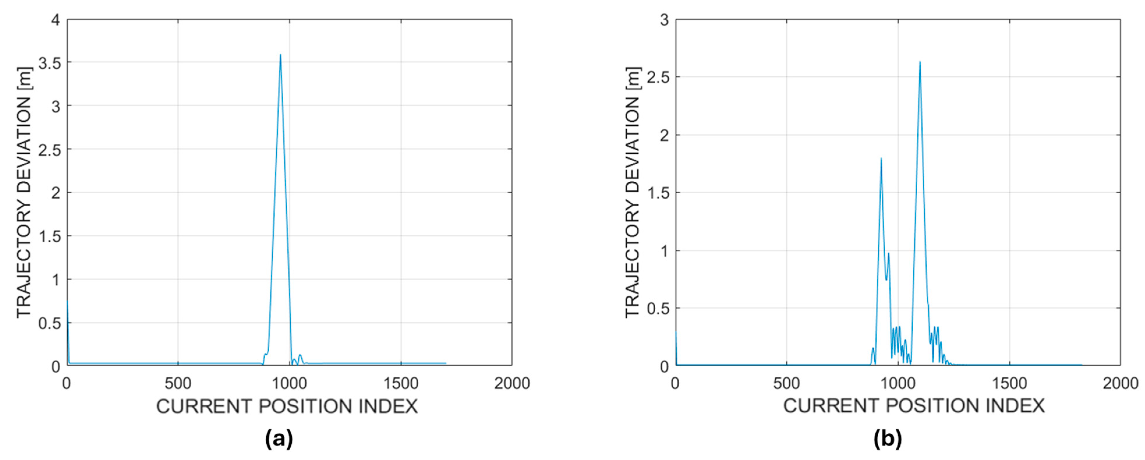
• Average trajectory deviation (ATD).
• Oscillating factor (OF).

For both the indicators, the concept of trajectory deviation is fundamental. For each position occupied by the rover, the trajectory deviation is defined as the distance between the vehicle and the nearest point of the trajectory determined though the path-planning phase. The average trajectory deviation (ATD) is equal to the mean value of the average trajectory deviation calculated for every position occupied by the rover. As it can be easily guessed, the lower the average trajectory deviation, the greater the efficiency of the algorithm. The oscillating factor (OF) indicator is used to evaluate if the steering corrections executed by the rover are appropriate or not for keeping itself on the planned trajectory. Considering the trajectory deviation of the rover during its mission, it can be observed that in the case of high steering correction, the deviation presents a wave-like trend. Otherwise, the trajectory deviation trend is smoother. The oscillating factor evaluation is performed counting the relative peaks of the trajectory deviation curve. Also, in this case, the lower the number of peaks, the greater the efficiency of the algorithm. In Figure 14, two examples of trajectory deviation curves with high and low steering corrections are reported for easier understanding.

The assessment of the autonomous driving algorithm was conducted by executing numerical simulations. In particular, given the characteristics of the rover, the were performed by evaluating the average trajectory deviation and the oscillating factor indexes. The range of LD considered was from 0.5 m to 2 m. Indeed, considering the typical dimensions of an orchard fruit row, for values outside this interval, the behavior of the rover can be considered non-compliant toward the mission that must be accomplished.

In Figure 15, the trends of the ATD as a function of the WPPs for different values of LD are reported.

In observing the chart, it emerges that the ATD is substantially constant at the different WPPs considered. On the other hand, the LD index plays a fundamental role in determining the average deviation. Indeed, it can be noted that, outside of a certain range of LD, namely from 0.5 to 1 m, the best performance cannot be obtained in terms of path adherence with respect to the ideal planned trajectory. In particular, high values of LD cause an increase in the ATD because the local goal point found by the rover is too far from its current position. As a consequence, the vehicle ignores the portion of path between itself and the local goal point, and it moves away from the ideal route. In the case of low values of LD, the local goal point is too close to rover current position. As a consequence, it starts to describe a pendulum-like trajectory in order to reach the local goal point, oscillating around the waypoint, as described in Figure 9b. The behavior of the rover is confirmed by observing the trend of the oscillating factor at different WPPs (Figure 16).

In the plot, it appears evident that with an increasing value of LD, the number of steering corrections decreases, and, therefore, the rover reduces the pendulum movement around the ideal trajectory, whereas the curve-cutting phenomena become more evident. This is clear in Figure 17.

Based on the results obtained in this study, a final indicator to evaluate the overall quality of how the rover pursuits the planned trajectory is proposed. It is called the relative accuracy (RA), and it can be determined through the following equation:

$$\mathrm{RA}=\frac{1}{(\mathrm{A}\mathrm{T}\mathrm{D}·\mathrm{O}\mathrm{F})}$$

(8)

This indicator is defined as “relative” because it is not possible to evaluate the quality of the autonomous driving algorithm in absolute terms since its performance depends on several factors, such as the main features of the vehicle, and the operative environment conditions. However, the RA can help to find the best combination of the factors that may influence the result. In Figure 18, the RA trend as a function of LD and WPP is reported.

Looking at the graph, it can be noted that the best performance of the vehicle can be obtained for an LD value of 0.75 m and WPP values between 0.16 and 0.66 m. This factor combination allows for obtaining RA values of 0.33–0.34 m⁻¹, which represent the maximum values obtained for the proposed study. This is also confirmed by observing the behavior of the vehicle during the execution of a hairpin turn for different values of RA (Figure 19).

Lastly, in Figure 20, the actual path followed by the rover along the entire map with respect to the planned one, corresponding to the max value of RA determined in this study, is shown.

The results obtained are quite interesting because they prove the possibility of implementing this kind of control logic on agricultural rovers equipped with this kind of powertrain. Furthermore, the proposed methodology may be a helpful instrument for farmers during the planning of a robot mission. The geographical coordinates of the outermost points of the orchard/vineyard can be used to build a cartesian system, like the one proposed in this study. In this way, given the geometrical features of the orchard and of the vehicle, it is possible to accurately tune the algorithm input parameters in order to generate the correct waypoint sequence, and the latter can successively be implemented in the rover during its mission profile definition.

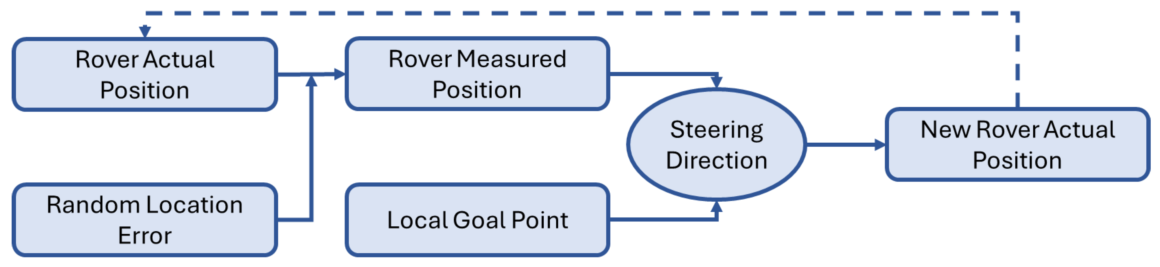
Influence of Positioning Error

In this sub-section, the impact of the location error on the algorithm reliability and precision is described. Indeed, almost every autonomous driven vehicle is equipped with a proper locating device, without which it is not able to find its way on the map. The devices based on GPS-RTK technology are the best performing because they are able to reach centimetric-level precision [55,56]. However, the position read by the device is not perfect but is affected by error, known as the accuracy. The accuracy indicates the maximum difference (expressed in meters) between the actual location of the rover and the one measured by the locating system.

In this study, the impact of the locating error was considered in evaluating the RA performance indicator, given a certain degree of accuracy. The baseline for the sensitivity analysis is represented by the best result obtained for the ideal case (WPP = 0.33 m, LD = 0.75 m, and RA = 0.34 m⁻¹). The simulations were carried out implementing, in the algorithm, a random error on the read rover position. The random error was proportional to the level of accuracy considered. The range of accuracy, considered for the analysis, was between 0.01 m and 0.1 m. It did not make sense to consider values outside of this range since they would not be applicable for real-case scenarios. The flowchart in Figure 21 helps to better understand the working principle of the location error in the algorithm.

The coordinates of the measured position are determined summing a random contribution, in the range of [− accuracy; + accuracy], to the ones that define the current position of the rover. In this way, it is possible to emulate the behavior of a GPS positioning device. If the accuracy level is set to 0, the obtained results correspond to the ideal case.

The obtained results in terms of the relative accuracy (RA) are reported in

Table 2. Impact of location error analysis results.

Accuracy (m)	RA (m−1)	∆RA % with Respect to Baseline
0 (baseline)	0.34	0%
±0.01	0.0272	−91.77%
±0.02	0.0317	−90.43%
±0.05	0.0316	−90.45%
±0.1	0.0273	−91.75%

.

It seems that with the introduction of a positioning error, the developed algorithm is not able to drive the vehicle along the path. However, in investigating the obtained results further, it emerged that the drop in the RA was due to a very strong rise in the value of the oscillating factor (OF). This growth was caused by a lot of steering angle micro-corrections because the vehicle always aims to follow the ideal trajectory. Micro-corrections are often very small and undetectable, and they are not the cause of an effective bad behavior of the rover during driving. This is more evident in observing the behavior of the rover during the execution of a hairpin turn (Figure 22).

However, this kind of behavior cannot be considered coherent with a real-case scenario: indeed, it is unthinkable that, in each cycle, which is in the order of milliseconds, the vehicle makes an infinitesimal steering correction. For this reason, a threshold value on the minimum steering angle was implemented in order to avoid micro-corrections. The obtained results with the updated model are shown in

Table 3. Impact of location error analysis results in the case of a 2.5° threshold on the steering angle.

Accuracy (m)	RA (m−1)	∆RA % with Respect to Baseline
0 (ideal case)	0.7232	118.4%
±0.01	0.6421	93.92%
±0.02	0.6219	87.80%
±0.05	0.3022	−8.74%
±0.1	0.0601	−81.85%

.

In observing the results, it emerges that the introduction of a cutoff value on the steering direction had a powerful effect on the improvement of the algorithm RA. Indeed, the results obtained are a lot better than the baseline case. Furthermore, it can be noted that the location error had low influence on the reliability of algorithm when the rover was equipped with the GPS-RTK positioning device and a fixed signal (accuracy range within 2 cm [57]).

4. Conclusions

In this work, an autonomous driving algorithm for a four-wheel differential-drive agricultural rover, operating in orchards or vineyards, has been proposed. The entire model was developed within the MATLAB software environment. After a brief description of the vehicle, a parametric procedure to build the operative environment was developed. The successive paragraphs focused on the autonomous driving algorithm, which is made up of two phases: path planning and path following. The aim of the first phase is to generate the path that the rover must follow in order to accomplish its mission. The path-planning algorithm is based on Dubins theory. The path-following phase consists of the control logic adopted by the vehicle in order to follow the planned route. The adopted strategy is inspired by the pure pursuit controller and consists of the definition of a local goal point and the command settings that must be implemented in the vehicle in order to reach the desired goal point. The obtained results underline that, by fixing the rover operative conditions, the algorithm performance could be influenced by two parameters: the lookahead distance (LD) and the waypoint pitch (WPP) distribution. To measure the reliability of the algorithm, two performance indicators were proposed in this article: the average trajectory deviation (ATD) and the oscillating factor (OF). The first one is linked to the overlap between the actual and planned paths. The second one is linked to the steering correction frequency carried out by the vehicle to follow the ideal trajectory. Then, a further indicator to identify the best tuning parameters, called the relative accuracy (RA), was defined. What emerged is that WPPs generally have low influence on the results. Instead, the algorithm reliability is strongly influenced by the LD value: indeed, it is necessary to determine the right balance because values of LD that are both too high and too low are not suitable. Finally, the impact of the location error of the rover on the algorithm efficiency was performed to enhance the applicability of this study also to real-world case scenarios. The simulation results underline the reliability of the algorithm when the accuracy of the rover positioning device is within 2 cm, which is the upper limit for GPS-RTK fixed-signal systems.

This work lays a foundation for interesting future developments. The introduction of a dynamic value of LD may lead to improved algorithm efficiency and computing time. The development of an adequate obstacle avoidance strategy represents a very important upgrade because, in this way, the rover will be able to avoid unexpected obstacles. At the same time, a field test campaign needs to be carried out. Indeed, performing experimental validation of the algorithm can lead to several benefits:

• Empirical assessment of the algorithm’s reliability.
• The introduction of possible corrective coefficients linked with the dynamic behavior of the rover.

Other developments are strictly connected with the algorithm itself but with the effects of sensor network with which the rover is equipped, such as the correlation between motion strategy and the tasks that the vehicle must perform in order to accomplish its mission.

References

1. FAO. World Food and Agriculture—Statistical Yearbook 2021; FAO: Rome, Italy, 2021; ISBN 978-92-5-134332-6. [Google Scholar]
2. Prosekov, A.Y.; Ivanova, S.A. Food Security: The Challenge of the Present. Geoforum 2018, 91, 73–77. [Google Scholar] [CrossRef]
3. Martelli, S.; Mocera, F.; Somà, A. Carbon Footprint of an Orchard Tractor through a Life-Cycle Assessment Approach. Agriculture 2023, 13, 1210. [Google Scholar] [CrossRef]
4. Mantoam, E.J.; Romanelli, T.L.; Gimenez, L.M. Energy Demand and Greenhouse Gases Emissions in the Life Cycle of Tractors. Biosyst. Eng. 2016, 151, 158–170. [Google Scholar] [CrossRef]
5. Martelli, S.; Mocera, F.; Somà, A. New Challenges towards Electrification Sustainability: Environmental Impact Assessment Comparison between ICE and Hybrid-Electric Orchard Tractor; SAE: Warrendale, PA, USA, 2023. [Google Scholar]
6. Wollenberg, E.; Richards, M.; Smith, P.; Havlík, P.; Obersteiner, M.; Tubiello, F.N.; Herold, M.; Gerber, P.; Carter, S.; Reisinger, A.; et al. Reducing Emissions from Agriculture to Meet the 2 °C Target. Glob. Chang. Biol. 2016, 22, 3859–3864. [Google Scholar] [CrossRef]
7. Gołasa, P.; Wysokiński, M.; Bieńkowska-Gołasa, W.; Gradziuk, P.; Golonko, M.; Gradziuk, B.; Siedlecka, A.; Gromada, A. Sources of Greenhouse Gas Emissions in Agriculture, with Particular Emphasis on Emissions from Energy Used. Energies 2021, 14, 3784. [Google Scholar] [CrossRef]
8. Clerici, D.; Martelli, S.; Mocera, F.; Somà, A. Mechanical Characterization of Lithium-Ion Batteries with Different Chemistries and Formats. J. Energy Storage 2024, 84, 110899. [Google Scholar] [CrossRef]
9. Platis, D.; Anagnostopoulos, C.; Tsaboula, A.; Menexes, G.; Kalburtji, K.; Mamolos, A. Energy Analysis, and Carbon and Water Footprint for Environmentally Friendly Farming Practices in Agroecosystems and Agroforestry. Sustainability 2019, 11, 1664. [Google Scholar] [CrossRef]
10. Stott, P.A.; Christidis, N.; Otto, F.E.L.; Sun, Y.; Vanderlinden, J.; van Oldenborgh, G.J.; Vautard, R.; von Storch, H.; Walton, P.; Yiou, P.; et al. Attribution of Extreme Weather and Climate-related Events. WIREs Clim. Change 2016, 7, 23–41. [Google Scholar] [CrossRef]
11. Patz, J.A.; Campbell-Lendrum, D.; Holloway, T.; Foley, J.A. Impact of Regional Climate Change on Human Health. Nature 2005, 438, 310–317. [Google Scholar] [CrossRef]
12. Ravankar, A.; Ravankar, A.A.; Rawankar, A.; Hoshino, Y. Autonomous and Safe Navigation of Mobile Robots in Vineyard with Smooth Collision Avoidance. Agriculture 2021, 11, 954. [Google Scholar] [CrossRef]
13. Liang, Y.; Zhou, K.; Wu, C. Environment Scenario Identification Based on GNSS Recordings for Agricultural Tractors. Comput. Electron. Agric. 2022, 195, 106829. [Google Scholar] [CrossRef]
14. Mocera, F.; Somà, A.; Martelli, S.; Martini, V. Trends and Future Perspective of Electrification in Agricultural Tractor-Implement Applications. Energies 2023, 16, 6601. [Google Scholar] [CrossRef]
15. Pascuzzi, S.; Łyp-Wrońska, K.; Gdowska, K.; Paciolla, F. Sustainability Evaluation of Hybrid Agriculture-Tractor Powertrains. Sustainability 2024, 16, 1184. [Google Scholar] [CrossRef]
16. Beligoj, M.; Scolaro, E.; Alberti, L.; Renzi, M.; Mattetti, M. Feasibility Evaluation of Hybrid Electric Agricultural Tractors Based on Life Cycle Cost Analysis. IEEE Access 2022, 10, 28853–28867. [Google Scholar] [CrossRef]
17. Martini, V.; Mocera, F.; Somà, A. Carbon Footprint Enhancement of an Agricultural Telehandler through the Application of a Fuel Cell Powertrain. World Electr. Veh. J. 2024, 15, 91. [Google Scholar] [CrossRef]
18. Martini, V.; Mocera, F.; Somà, A. Design and Experimental Validation of a Scaled Test Bench for the Emulation of a Hybrid Fuel Cell Powertrain for Agricultural Tractors. Appl. Sci. 2023, 13, 8582. [Google Scholar] [CrossRef]
19. Al-lwayzy, S.; Yusaf, T. Chlorella Protothecoides Microalgae as an Alternative Fuel for Tractor Diesel Engines. Energies 2013, 6, 766–783. [Google Scholar] [CrossRef]
20. Owczuk, M.; Matuszewska, A.; Kruczyński, S.; Kamela, W. Evaluation of Using Biogas to Supply the Dual Fuel Diesel Engine of an Agricultural Tractor. Energies 2019, 12, 1071. [Google Scholar] [CrossRef]
21. Baillie, C.P.; Thomasson, J.A.; Lobsey, C.R.; McCarthy, C.L.; Antille, D.L. A Review of the State of the Art in Agricultural Automation. Part I: Sensing technologies for optimization of machine operation and farm inputs. In Proceedings of the 2018 ASABE Annual International Meeting, Detroit, MI, USA, 29 July–1 August 2018; American Society of Agricultural and Biological Engineers: St. Joseph, MI, USA, 2018. [Google Scholar]
22. Ghobadpour, A.; Boulon, L.; Mousazadeh, H.; Malvajerdi, A.S.; Rafiee, S. State of the Art of Autonomous Agricultural Off-Road Vehicles Driven by Renewable Energy Systems. Energy Procedia 2019, 162, 4–13. [Google Scholar] [CrossRef]
23. Roshanianfard, A.; Noguchi, N.; Okamoto, H.; Ishii, K. A Review of Autonomous Agricultural Vehicles (The Experience of Hokkaido University). J. Terramech. 2020, 91, 155–183. [Google Scholar] [CrossRef]
24. Rubio, F.; Valero, F.; Llopis-Albert, C. A Review of Mobile Robots: Concepts, Methods, Theoretical Framework, and Applications. Int. J. Adv. Robot. Syst. 2019, 16, 172988141983959. [Google Scholar] [CrossRef]
25. Durmus, H.; Gunes, E.O.; Kirci, M.; Ustundag, B.B. The Design of General Purpose Autonomous Agricultural Mobile-Robot: “AGROBOT”. In Proceedings of the 2015 Fourth International Conference on Agro-Geoinformatics (Agro-Geoinformatics), Istanbul, Turkey, 20–24 July 2015; pp. 49–53. [Google Scholar]
26. Califano, F.; Cosenza, C.; Niola, V.; Savino, S. Multibody Model for the Design of a Rover for Agricultural Applications: A Preliminary Study. Machines 2022, 10, 235. [Google Scholar] [CrossRef]
27. Sparrow, R.; Howard, M. Robots in Agriculture: Prospects, Impacts, Ethics, and Policy. Precis. Agric. 2021, 22, 818–833. [Google Scholar] [CrossRef]
28. Pedersen, S.M.; Fountas, S.; Have, H.; Blackmore, B.S. Agricultural Robots—System Analysis and Economic Feasibility. Precis. Agric. 2006, 7, 295–308. [Google Scholar] [CrossRef]
29. King, A. Technology: The Future of Agriculture. Nature 2017, 544, S21–S23. [Google Scholar] [CrossRef] [PubMed]
30. Yahya, N. Green Urea; Springer: Singapore, 2018; ISBN 978-981-10-7577-3. [Google Scholar]
31. Martelli, S.; Mocera, F.; Somà, A. Co-Simulation of a Specialized Tractor for Autonomous Driving in Orchards; SAE: Warrendale, PA, USA, 2022. [Google Scholar]
32. Han, J.; Park, C.; Jang, Y.Y.; Gu, J.D.; Kim, C.Y. Performance Evaluation of an Autonomously Driven Agricultural Vehicle in an Orchard Environment. Sensors 2021, 22, 114. [Google Scholar] [CrossRef] [PubMed]
33. Ko, M.H.; Ryuh, B.-S.; Kim, K.C.; Suprem, A.; Mahalik, N.P. Autonomous Greenhouse Mobile Robot Driving Strategies From System Integration Perspective: Review and Application. IEEE/ASME Trans. Mechatron. 2015, 20, 1705–1716. [Google Scholar] [CrossRef]
34. Santos, L.C.; Santos, F.N.; Solteiro Pires, E.J.; Valente, A.; Costa, P.; Magalhaes, S. Path Planning for Ground Robots in Agriculture: A Short Review. In Proceedings of the 2020 IEEE International Conference on Autonomous Robot Systems and Competitions (ICARSC), Ponta Delgada, Portugal, 15–17 April 2020; pp. 61–66. [Google Scholar]
35. Han, X.; Lai, Y.; Wu, H. A Path Optimization Algorithm for Multiple Unmanned Tractors in Peach Orchard Management. Agronomy 2022, 12, 856. [Google Scholar] [CrossRef]
36. Hameed, I.A. Intelligent Coverage Path Planning for Agricultural Robots and Autonomous Machines on Three-Dimensional Terrain. J. Intell. Robot. Syst. 2014, 74, 965–983. [Google Scholar] [CrossRef]
37. Santos, L.; Santos, F.; Mendes, J.; Costa, P.; Lima, J.; Reis, R.; Shinde, P. Path Planning Aware of Robot’s Center of Mass for Steep Slope Vineyards. Robotica 2020, 38, 684–698. [Google Scholar] [CrossRef]
38. Bochtis, D.; Griepentrog, H.W.; Vougioukas, S.; Busato, P.; Berruto, R.; Zhou, K. Route Planning for Orchard Operations. Comput. Electron. Agric. 2015, 113, 51–60. [Google Scholar] [CrossRef]
39. Juman, M.A.; Wong, Y.W.; Rajkumar, R.K.; H’ng, C.Y. An Integrated Path Planning System for a Robot Designed for Oil Palm Plantations. In Proceedings of the TENCON 2017—2017 IEEE Region 10 Conference, Penang, Malaysia, 5–8 November 2017; pp. 1048–1053. [Google Scholar]
40. Li, S.; Xu, H.; Ji, Y.; Cao, R.; Zhang, M.; Li, H. Development of a Following Agricultural Machinery Automatic Navigation System. Comput. Electron. Agric. 2019, 158, 335–344. [Google Scholar] [CrossRef]
41. Hernandez, J.I.; Kuo, C.Y. Steering Control of Automated Vehicles Using Absolute Positioning Gps and Magnetic Markers. IEEE Trans. Veh. Technol. 2003, 52, 150–161. [Google Scholar] [CrossRef]
42. Huang, P.; Luo, X.; Zhang, Z. Headland Turning Control Method Simulation of Autonomous Agricultural Machine Based on Improved Pure Pursuit Model. In Computer and Computing Technologies in Agriculture III, Proceedings of the Third IFIP TC 12 International Conference, CCTA 2009, Beijing, China, 14–17 October 2009; Springer: Berlin/Heidelberg, Germany, 2010; pp. 176–184. [Google Scholar]
43. Peng, H.; Wang, W.; An, Q.; Xiang, C.; Li, L. Path Tracking and Direct Yaw Moment Coordinated Control Based on Robust MPC With the Finite Time Horizon for Autonomous Independent-Drive Vehicles. IEEE Trans. Veh. Technol. 2020, 69, 6053–6066. [Google Scholar] [CrossRef]
44. Sainz-Rubio, V.; Rovira-Mas, F.; Diago, M.P.; Fernandez-Novales, J.; Barrio, I.; Cuenca, A.; Alves, F.; Valente, J.; Tardaguila, J. VINESCOUT: A Vineyard Autonomous Robot for on-the-Go Assessment of Grapevine Vigour and Water Status. Available online: https://investigacion.unirioja.es/documentos/603618dcd700765ec201af64/f/60362b47d700765ec201af65.pdf (accessed on 19 May 2024).
45. Fountas, S.; Mylonas, N.; Malounas, I.; Rodias, E.; Hellmann Santos, C.; Pekkeriet, E. Agricultural Robotics for Field Operations. Sensors 2020, 20, 2672. [Google Scholar] [CrossRef]
46. Gobhinath, S.; Darshini, M.D.; Durga, K.; Priyanga, R.H. Smart Irrigation with Field Protection and Crop Health Monitoring System Using Autonomous Rover. In Proceedings of the 2019 5th International Conference on Advanced Computing & Communication Systems (ICACCS), Coimbatore, India, 15–16 March 2019; pp. 198–203. [Google Scholar]
47. Cornejo, J.; Magallanes, J.; Denegri, E.; Canahuire, R. Trajectory Tracking Control of a Differential Wheeled Mobile Robot: A Polar Coordinates Control and LQR Comparison. In Proceedings of the 2018 IEEE XXV International Conference on Electronics, Electrical Engineering and Computing (INTERCON), Lima, Peru, 8–10 August 2018; pp. 1–4. [Google Scholar]
48. Korkmaz, M.; Durdu, A. Comparison of Optimal Path Planning Algorithms. In Proceedings of the 2018 14th International Conference on Advanced Trends in Radioelecrtronics, Telecommunications and Computer Engineering (TCSET), Lviv-Slavske, Ukraine, 20–24 February 2018; pp. 255–258. [Google Scholar]
49. Gasparetto, A.; Boscariol, P.; Lanzutti, A.; Vidoni, R. Path Planning and Trajectory Planning Algorithms: A General Overview. In Motion and Operation Planning of Robotic Systems: Background and Practical Approaches; Springer: Cham, Switzerland, 2015; pp. 3–27. [Google Scholar]
50. Dubins, L.E. On Curves of Minimal Length with a Constraint on Average Curvature, and with Prescribed Initial and Terminal Positions and Tangents. Am. J. Math. 1957, 79, 497. [Google Scholar] [CrossRef]
51. Hameed, I.A. Coverage Path Planning Software for Autonomous Robotic Lawn Mower Using Dubins’ Curve. In Proceedings of the 2017 IEEE International Conference on Real-Time Computing and Robotics (RCAR), Okinawa, Japan, 14–18 July 2017; pp. 517–522. [Google Scholar]
52. Macenski, S.; Singh, S.; Martín, F.; Ginés, J. Regulated Pure Pursuit for Robot Path Tracking. Auton. Robots 2023, 47, 685–694. [Google Scholar] [CrossRef]
53. Wang, W.-J.; Hsu, T.-M.; Wu, T.-S. The Improved Pure Pursuit Algorithm for Autonomous Driving Advanced System. In Proceedings of the 2017 IEEE 10th International Workshop on Computational Intelligence and Applications (IWCIA), Hiroshima, Japan, 11–12 November 2017; pp. 33–38. [Google Scholar]
54. Mocera, F.; Martini, V.; Somà, A. Comparative Analysis of Hybrid Electric Architectures for Specialized Agricultural Tractors. Energies 2022, 15, 1944. [Google Scholar] [CrossRef]
55. Mekik, C.; Arslanoglu, M. Investigation on Accuracies of Real Time Kinematic GPS for GIS Applications. Remote Sens. 2009, 1, 22–35. [Google Scholar] [CrossRef]
56. Ekaso, D.; Nex, F.; Kerle, N. Accuracy Assessment of Real-Time Kinematics (RTK) Measurements on Unmanned Aerial Vehicles (UAV) for Direct Geo-Referencing. Geo-Spat. Inf. Sci. 2020, 23, 165–181. [Google Scholar] [CrossRef]
57. Xu, H. Application of GPS-RTK Technology in the Land Change Survey. Procedia Eng. 2012, 29, 3454–3459. [Google Scholar] [CrossRef]
Figure 1. Top view schematic representation of the rover (a), and its equivalent kinematic model (b).
Agriengineering 06 00113 g001
Figure 3. Examples of different configurations of orchards obtained with the parametric model.
Agriengineering 06 00113 g003
Figure 5. Examples of path planning trajectories for different orchard configurations obtained with the parametric model. The red stars on the map represent the checkpoints.
Agriengineering 06 00113 g005
Figure 6. Path-planned trajectories obtained for the orchard configuration used in this study. The red stars on the map represent the checkpoints.
Agriengineering 06 00113 g006
Figure 7. Path-planning control logic.
Agriengineering 06 00113 g007
Figure 8. Representation of the path-following algorithm operating principle.
Agriengineering 06 00113 g008
Figure 9. Influence of lookahead distance: (a) the LD value is too high; (b) the LD value is too small.
Agriengineering 06 00113 g009
Figure 10. Possible scenarios of the interaction between the vehicle circumference and the waypoints: (a) no interaction; (b) intersection outside the waypoint segments; (c) single valid intersection; (d) multiple valid intersections.
Agriengineering 06 00113 g010
Figure 11. Simultaneous interaction between the rover circumference and several waypoint segments.
Agriengineering 06 00113 g011
Figure 13. Comprehensive flowchart of the motion strategy adopted by the agricultural rover.
Agriengineering 06 00113 g013
Figure 14. Trajectory deviation curves during the execution of a hairpin turn: (a) typical trend in cases of large steering corrections, (b) typical trend in cases of low steering corrections.
Agriengineering 06 00113 g014
Figure 15. ATD vs. WPP plot for different values of LD.
Agriengineering 06 00113 g015
Figure 16. OF vs. WPP plot for different values of LD.
Agriengineering 06 00113 g016
Figure 17. Hairpin turn trajectory: (a) LD = 0.5 m and WPP = 1.65 m; (b) LD = 0.5 m and WPP = 1.65 m.
Agriengineering 06 00113 g017
Figure 18. RA trend as a function of LD and WPP; the best results match with the highest values of RA because it means that the trajectory deviation and the pendulum-like movement along the ideal path are lower.
Agriengineering 06 00113 g018
Figure 19. Examples of hairpin turn execution for different values of RA: (a) 0.13 m−1; (b) 0.21 m−1; (c) 0.34 m−1.
Agriengineering 06 00113 g019
Figure 20. Actual path of the rover with an LD equal to 0.75 m, WPP equal to 0.33 m, and RA equal to 0.34 m−1.
Agriengineering 06 00113 g020
Figure 21. Working principle of location error assessment.
Agriengineering 06 00113 g021
Figure 22. Examples of hairpin turn execution for different values of position accuracy: (a) 0 m (baseline), (b) 0.1 m.
Agriengineering 06 00113 g022