Abstract
The field capacity (FC) and permanent wilting point (PWP) are fundamental hydrological properties critical for assessing water availability within soils, rather than direct measures of soil health. Due to the challenges associated with their field measurement, alternative assessment methods are necessary. In this study, global-scale accessible soil data were retrieved from the world soil database called the World Soil Information Service (WoSIS), and artificial neural network (ANN) and gene-expression programming (GEP) algorithms were used to predict soil FC and PWP based on easily obtainable parameters from the database. The best-fit variable combination for FC (longitude, latitude, altitude, sand content, silt content, clay content, and electrical conductivity) and PWP (best-fit FC combination plus pH) modeling was determined. Both ANN and GEP showed greater accuracy than linear-based models in simulating the FC and PWP from the best-fit variables. The mean absolute error (MAE) was reduced by 51.54% for the FC and 56.38% for the PWP by the ANN model, compared with the linear model used in the previous literature. The normalized root mean square error (NRMSE) evaluation indicated that the ANN model performed best for PWP prediction (NRMSE of 19.9%), while the GEP model was superior for FC prediction (NRMSE of 29.9%). Between the ANN and GEP models, the ANN model showed a slightly higher model of interpretability; however, the GEP model exhibited a similar or better ability to avoid large error, based on the error distribution. Overall, our results demonstrated that machine learning is effective in predicting the FC and PWP from easily accessible data from WoSIS, and the GEP model is more preferable for FC and PWP modeling.
1. Introduction
Plant available water capacity provides information on the amount of water that is stored in soil and can be used by plants, which is determined by the differences between the soil field capacity (FC, −33 kPa of suction pressure) and the permanent wilting point (PWP, −1500 kPa of suction pressure) [1]. While the FC and PWP are critical for understanding soil water dynamics, it is important to clarify that these parameters primarily reflect the hydrological aspects of soil rather than direct measures of soil health. These properties are integral to applications such as irrigation management [2], crop modeling [3], and precision agriculture [4]. However, the FC and PWP of soil are often not available because their measurements are both time-consuming and costly [5,6]. In the latest soil health database, SoilHealthDB [7], only 81 results for the FC and PWP were reported out of 5908 data entries across 41 countries. This paucity of direct data underscores the urgent need for more efficient and cost-effective methodologies to estimate these crucial soil parameters. Therefore, the capability to estimate the FC and PWP from other easily measurable parameters is highly desirable [8]. Historically, pedotransfer functions (PTFs) have been applied to derive FC and PWP values based on parameters like soil texture, soil bulk density, and soil organic matter (SOM) [9,10]. These traditional methods, while noble in their intent, have been fraught with challenges, most prominently their limited accuracy. In an innovative push to enhance the precision of these models, parameters like the soil cation exchange capacity (CEC) [11], soil calcium carbonate (CaCO3) content [12], geographical locations [13], and even geographical nuances [13] have been incorporated. Past efforts have shed light on the limitations of conventional models. For instance, Santra et al. [9] calculated the gravimetric FC and PWP in arid western India with sand, silt, and clay contents; organic carbon; and bulk density as input variables of PTF. The results showed that the coefficient of determination (R2) of best-fit FC and PWP was 0.63 and 0.34, respectively. Cueff et al. [14] used CEC and phosphorus content as additional inputs in addition to those used by Santra and colleagues to model the FC and PWP for soil in southwest France. The root mean squared error (RMSE) of their model ranged from 3.7% to 8.0% for the FC and 3.4% to 5.7% for the PWP. A significant drawback of previous efforts is the reliance on linear algorithms, which have inherently restricted the accuracy of these models [15,16].
Considering these challenges, there is a clear and present need for novel methodologies that move beyond traditional linear models, incorporating advanced algorithms that can capture the complexity and variability of soils, leading to more accurate and reliable estimations of the FC and PWP. For example, geostatistical approaches such as Kriging [17] and k-nearest neighbors (k-NN) [18] and parameter approaches such as regression tree (RT) [16], artificial neural network (ANN) [19], neuro-fuzzy (NF) [20], random forest (RF) [21], support vector machine (SVM) [22], gene-expression programming (GEP) [20], and deep learning (DL) [23] have been used for FC and PWP modeling in various studies. In a recent study, Shiri et al. [20] modeled FC and PWP for soil in Iran (0–60 cm) using five different algorithms: SVM, GEP, NF, RF, and RT. The contents of sand, silt, and clay; equivalent CaCO3; bulk density; particle density; geometric mean of particle diameter; and geometric standard deviation of soil particle size were used as input variables. The study findings showed that the NF model had the highest R2 followed by GEP. Taşan and Demir [12] simulated the FC and PWP in Turkey by conventional linear regression (REG) and an ANN, with sand, silt, and clay contents; bulk density; OM; CEC; and CaCO3 as input variables. The results showed that the ANN model displayed higher modeling accuracy, and R2, RMSE, and the mean absolute error (MAE) were 0.80, 3.12%, and 2.27% for the FC and 0.83, 1.84%, and 2.40% for the PWP, respectively. Yamaç et al. [23] modeled the FC and PWP of soil in Turkey using previously published PTFs, as well as k-NN, DL, and ANN using the same input data of sand, silt, and clay content; lime; bulk density; OM; particle density; and aggregate stability. The DL and ANN approaches had comparable R2 and MAE values of 0.829 and 2.7% in the FC modeling. In PWP modeling, k-NN showed the best performance with an R2 = 0.800 and MAE = 2.1%. Although previous studies demonstrated remarkable FC and PWP modeling ability by advanced algorithms, they were primarily based on site-specific datasets [14,24]. Therefore, models that can be applied to broader geographical regions are still missing.
Due to the importance of the FC and PWP in agricultural production, more reliable and broadly applicable FC and PWP modeling based on global-scale soil datasets is needed [12,13,14,23]. This study leveraged machine learning (ML) algorithms, specifically ANN and GEP, to predict FC and PWP values using an extensive range of data. The models incorporated physical (sand, silt, and clay content), chemical (electrical conductivity (EC) and pH), and geological (longitude, latitude, and altitude) parameters. Both EC and pH were found to be significantly related to soil water content (SWC) [25,26] and are easy to measure [27,28], but they were not used as modeling inputs in previous FC and PWP simulations.
ANNs were chosen for their proven ability to handle complex, non-linear interactions and large datasets, which makes them ideal for analyzing intricate relationships among various soil properties. Their effectiveness is supported by research that highlights their utility in modeling diverse soil dynamics, such as soil compaction and water retention [29,30]. Conversely, GEP was selected for its strengths in modeling non-linear and complex interactions, including soil water capacity [20] and soil stability [31], offering a robust framework for scenarios where traditional models may falter. This adaptability is crucial for fine-tuning models to uncover subtle patterns and interactions in the soil data. By integrating these advanced algorithms, this study aimed to enhance the predictive accuracy of FC and PWP models, providing a more comprehensive understanding of soil behavior that is critical for improving agricultural practices and irrigation strategies. The inclusion of ANNs and GEP represents a significant advancement over conventional linear models, offering new insights into soil dynamics that could lead to more effective and environmentally sustainable agricultural outcomes. Specific objectives of this study included the following:
- (i)
- Determine the optimal combination of variables for FC and PWP modeling;
- (ii)
- Apply machine learning algorithms to predict the FC and the PWP from easily measurable inputs from global scale accessible data.
2. Materials and Methods
2.1. Data Source and Process
Both the FC and PWP (cm3/100 cm3; %) and related soil composition (sand, silt, and clay contents; %), geographical location (longitude, latitude; decimal degree), pH, and EC (dS/m) were retrieved from the latest global soil database (WoSIS) [32]. Another geographical variable, altitude (m), was retrieved from Google Maps by the longitude and latitude information of the sample site. The WoSIS database includes over 5.8 million quality-assessed records from 173 countries. The procedure for data standardization and detailed information on the WoSIS database can be found in [32,33,34]. In this study, the WoSIS data were cleaned by only keeping information on the topsoil from 0 to 35 cm and by using a dataset that had complete information on the input variables, the FC, and the PWP. A total of 210 FC and 254 PWP values were extracted from the database for modeling. Descriptive statistical information for FC and PWP modeling, including the average (μ), standard deviation (σ), maximum (Max.) and minimum (Min.) of all used variables, and correlation coefficient (r) between each input variable and the FC or PWP, are summarized in Table 1. The geographical distribution of the FC and PWP from the database are shown in Figure 1. The soil classification and countries from which the applied dataset for FC and PWP modeling were derived are shown in the Appendix A Table A1. The boxplot-based dataset distribution is illustrated in Figure A1.

Table 1.
Values of the input parameters for model fitting.

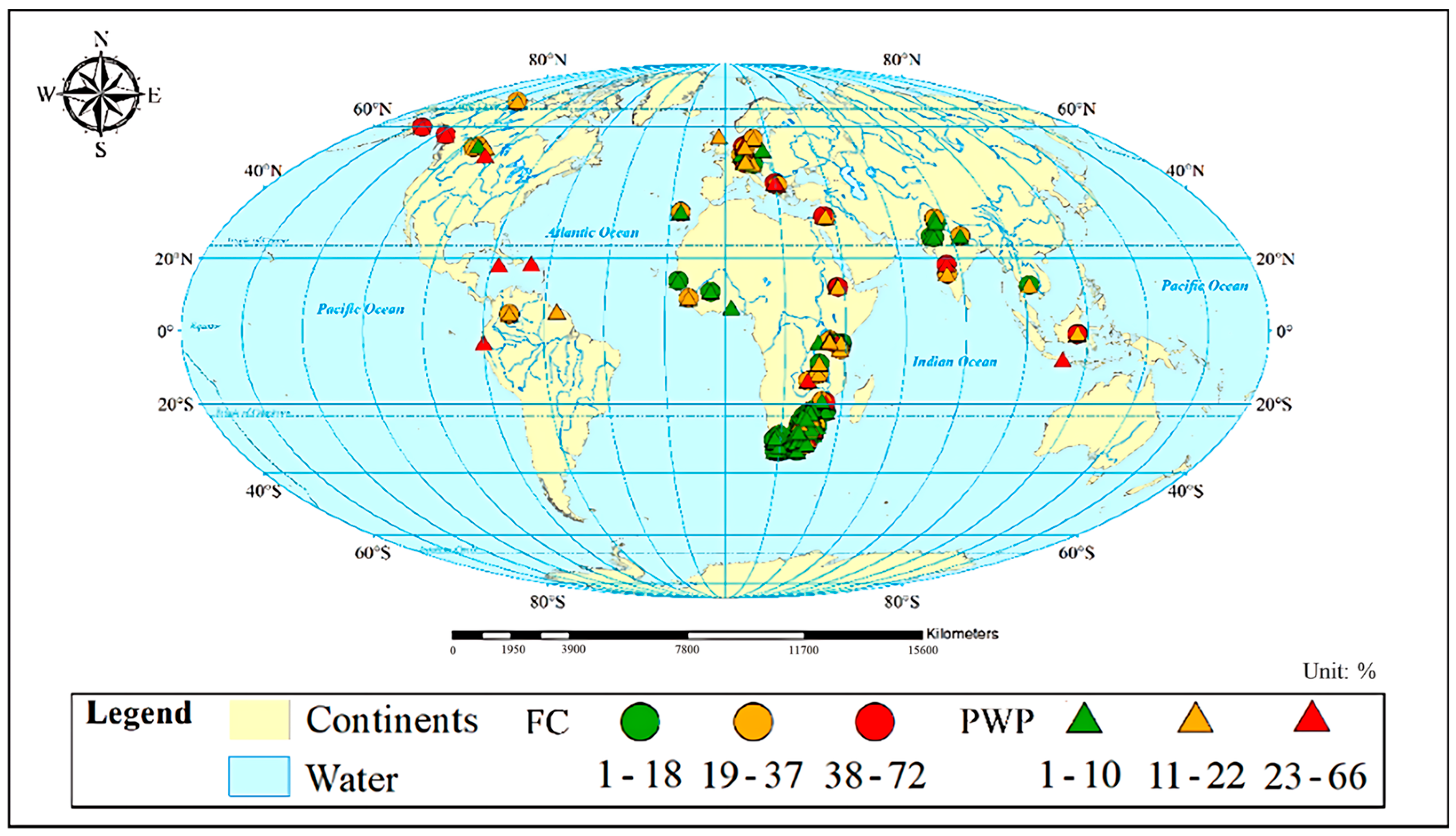
Figure 1.
Geographic origin of the samples in the modeling dataset. Circle symbols represent the field capacity (FC) and triangle symbols stand for the permanent wilting point (PWP). Different colors indicate the range of data values of the FC or PWP.
2.2. Previous PTFs and Linear Regression Algorithm
Three regression-based PTFs applied in Saxton and Rawls [35], Adhikary et al. [36], and Tóth et al. [16] were collected as base models for FC and PWP modeling (Appendix B, Table A3). In addition, this study developed a WoSIS-based PTF model based on a linear regression algorithm, which is described as Equation (1).
where n is the total number of data points, xi is the ith input variable; α is the slope of the linear equation; β is an intercept of the regression, and ε is the error term.
2.3. Artificial Neural Networks (ANNs)
In addition to the four linear regression-based models, two ML-enabled algorithms, ANN and GEP, were also evaluated for their predictive accuracy of the FC and PWP. ANN is a powerful algorithm for non-linear problems that performs experience-based learning processes with an inherent punishment mechanism. Compared with a conventional linear model, an ANN deploys data features in multiple dimensions, which enables more comprehensive and accurate predictions. This study used NeuroSolution 7.1 software (NeuroDimension Inc, Gainesville, FL, USA) to develop predictive models for the FC and PWP by using a classic backpropagation neural network (BPNN). The maximum epoch was 1000 and the algorithm had a 0.01 learning rate. The Levenberg–Marquardt gradient search method with an early stopping callback was used to prevent overfitting. A single hidden layer was employed with 10 neuros [37]. The modeling dataset was normalized using Equation (2) and randomly divided into three sub-datasets for training, cross-validation (CV), and testing, with data ratios of 70%, 15%, and 15%, respectively. The training dataset was used for initial model development, and the CV dataset was used for hyper-parameter adjustment; the adjusted model was applied to the testing dataset for model performance evaluation [38]. Cross-validation was unavailable in the linear regression (REG) model; therefore, the dataset for CV was added to the training set for REG modeling. The data ratio of training and testing of the REG model was 85% and 15%, respectively.
where xnorm is the normalized dimensionless variable, x is the observed value, xmin is the minimum observed value, and xmax is the maximum observed value of the variable.
2.4. Gene-Expression Programming (GEP)
The GEP algorithm was the second ML-based algorithm investigated in this study. The algorithm is capable of establishing mathematical relationships between input variables and output parameters, similar to the gene algorithm (GA) and gene programming (GP). However, the computing is significantly faster and the computer accuracy is appreciably higher than the GA and GP [39]. A classic GEP begins with a major race and undergoes a continuous evolutionary process, such as selection, replication, mating, mutation, adaptation, reversal, and transformation to evolve toward a predetermined objective [40,41,42]. In this study, GeneXproTools 5.0 software (Gepsoft Ltd., Bristol, UK) was used for FC and PWP modeling. The algorithm was also trained, cross-validated, and tested by the same input dataset as the ANN model. The FC model incorporates two genes, whereas the PWP model is more intricate, encompassing five genes. The process of gene linkage, or how these genes interact and combine, is pivotal. For the FC model, a “minimum” linking function is employed, signifying that the smallest value or output from its genes is selected. Conversely, the PWP model utilizes a “multiplication” linking function, indicating that the outputs of its genes are multiplied together to produce a resultant value. Ten head sizes were used for both models with fifty chromosomes and ten thousand evolved generations with model elements including +, −, *,/, x−1, x2, x5, x1/3, x1/4, x1/5, natural log (ln), floor, power, no processing, sine, cosine, tangent, arcsine, arctangent, average, and minimum. These operational elements, which can be likened to mathematical and computational functions, are integral to the model’s ability to adapt, learn, and ultimately solve the designated problem. Other parameters, such as the mutation rate, inversion rate, and gene transposition rate were set at default values, as described in the GEP theory in [43].
2.5. Assessment of the Best-Fit Combination of Input Variables for ML Based Models
The best-fit input variables for FC and PWP prediction using ML-based algorithms were determined using an ANN. Fifteen different combinations of input variables, including geographical location (L; longitude, latitude, and altitude), soil textures (S; sand, silt, and clay content), pH, EC, L + S, pH + EC, L + pH, L + EC, L + pH + EC, S + pH, S + EC, S + pH + EC, L + S + pH, L + S + EC, and L + S + pH + EC were evaluated. These combinations were used as input variables for ANN and typical model evaluation metrics, R2, RMSE, normalized RMSE (NRMSE), and MAE [44,45,46], were calculated to determine the model performance of each combination, as shown in Equation (3)–(6). Furthermore, following the approach of Jamieson et al. [47], the NRMSE was categorized into four classes: simulations with NRMSE less than 10% were deemed excellent, those between 10% and 20% were good, those between 20% and 30% were fair, and those above 30% were considered poor.
where R2 is the coefficient of determination, is the predicted value in ith datum, is the observed value in ith datum, is the average of the observations, n is the number of actual observations, RMSE is the root mean square error, NRMSE is normalized RMSE, MAE is the mean absolute error, and AE is the absolute error.
For the four linear models, Adhikary’s model [36] only used soil texture (sand, silt, and clay content) data as input variables, but the other two linear models required both OM and soil texture for modeling, which were also retrieved from the WoSIS database. A total of 210 data for the FC and 254 data for the PWP were used in the REG model and in Adhikary’s model. A total of 179 data in the FC and 219 data in the PWP were used in models in Saxton and Rawls [35] and Tóth et al. [16], the same as the dataset used in the REG, ANN, and GEP approaches in this study.
2.6. Rank the Input Variables for FC and PWP Modeling
The test dataset used for the FC and PWP simulation with ML models was evaluated by a Kolmogorov–Smirnov nonparametric test (K-S test) to determine the relative importance of input variables. The K-S test is a nonparametric test method for two sample comparison, which is unrelated to the sample’s frequency distribution and was used to compare the underlying probability distributions. The K-S test was analyzed by IBM SPSS software, version 22 (IBM Corp., Armonk, NY, USA). The test dataset was divided into 2 groups by MAE, with one group having an absolute error between observed targets and simulated results greater than MAE and the other group being smaller than MAE.
3. Results and Discussion
3.1. Determination of the Best-Fit Variables
To systematically elucidate the criteria behind the selection of variable combinations for FC and PWP modeling, our approach was grounded in a comprehensive analysis of soil properties’ interactions and their predictive significance. The modeling results from combinations of different inputs are shown in Table 2. The selection process was rigorously informed by a review of the existing literature and empirical evidence demonstrating the individual and combined effects of these properties on soil hydrology. In the FC model, the combination of L + S + EC resulted in the best performance. In the PWP simulation, L + S + pH + EC led to the highest accuracy. While the individual L and S datasets appeared to generate reasonable FC and PWP predictions, the combination of L + S generated more accurate FC and PWP simulations. Interestingly, while the model performance using ionic strength or EC alone as the input variable was quite low, their combination with L + S significantly enhanced the model performance in predicting both the FC and PWP. Previous studies suggested that EC is more sensitive to soil water variation [48,49] because the relative dielectric permittivity of water is generally more than an order of magnitude larger than that of other soil components [50]. As a result, the bulk relative dielectric permittivity of soil is primarily a function of the soil water content (SWC) [51]. The pH appears to have lower impact on the FC than the PWP, because the SWC easily fluctuates with the salinity content in the environment [52]. Chronically high or low pH has been found to cause soil water storage variation [26], but the SWC does not significantly change with rapidly varying pH. In addition, pH in the environment is relatively stable due to the carbonate buffering capacity, thus, its impact on SWC is not significant [53].
Table 2.
Performance of FC and PWP modeling by ANN using combinations of input variables.
3.2. Comparison of Simulated FC and PWP by Different Models
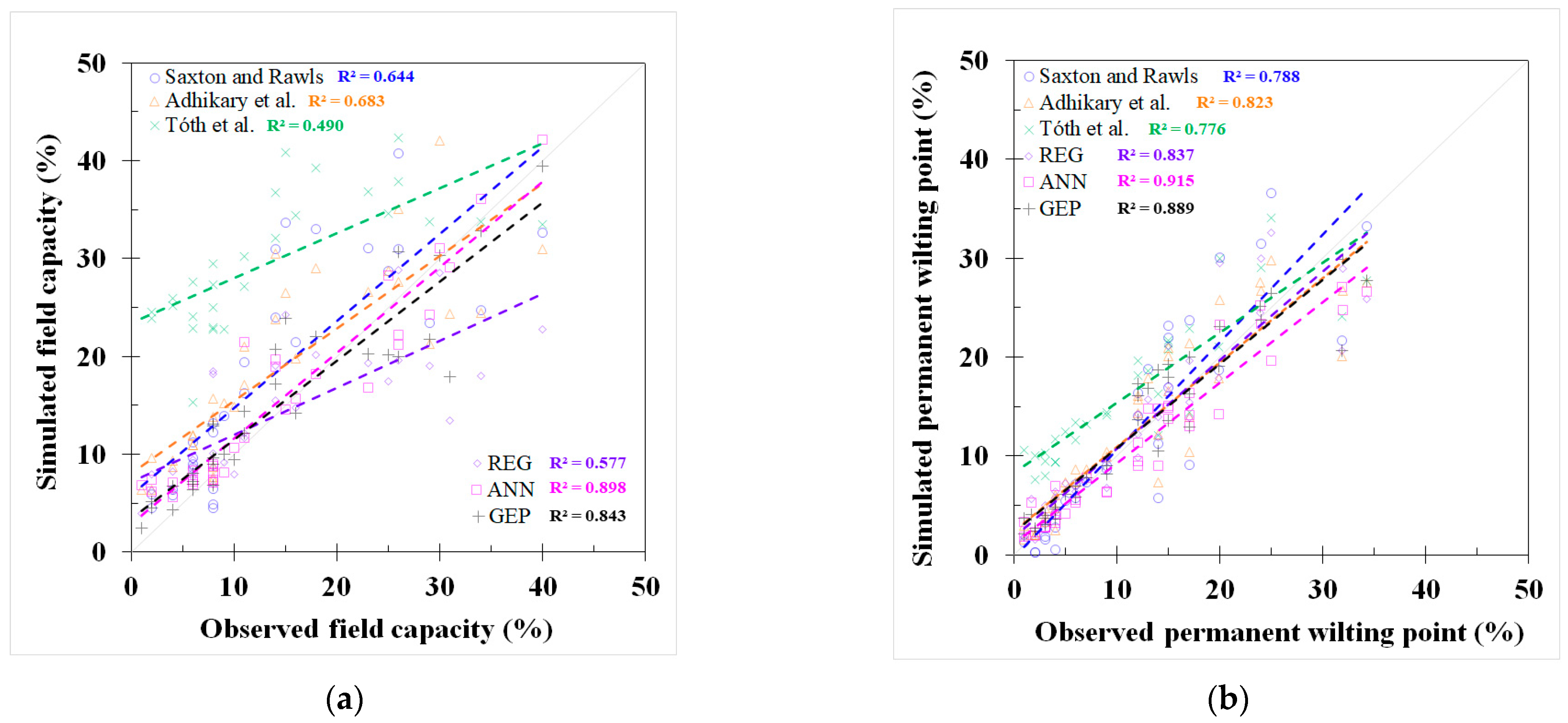
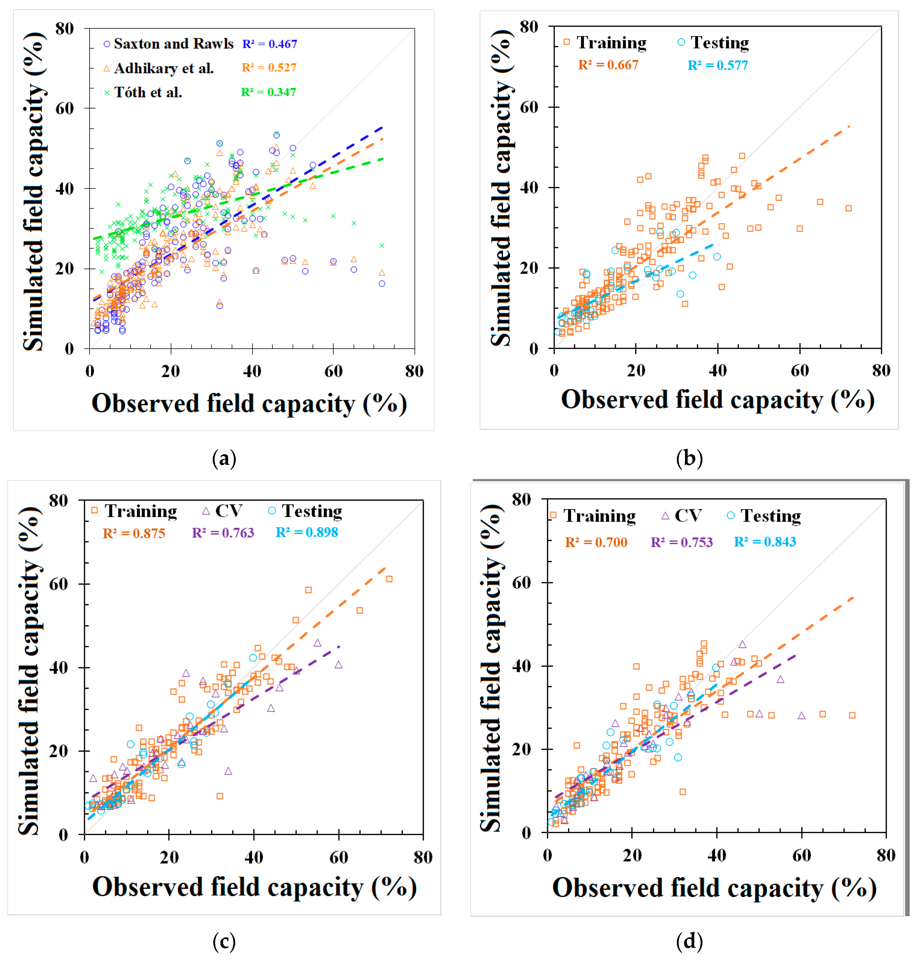
GEP and REG models were developed based on the best-fit combination identified above. As a comparison, the same set of data used for these models was also applied to three PTFs from the literature mentioned earlier (i.e., Saxton and Rawls, Adhikary et al., and Tóth et al.). The outputs from the published PTFs, REG, ANN, and GEP models, are shown in Figure 2 and Figure 3 and Appendix C, Table A4, respectively. The results showed that the model used in Adhikary et al. [36] has the highest R2 in the published PTF in both the FC (0.683) and the PWP (0.823) simulation. In the ANN, GEP, and REG models, the ANN performed the best, as indicated by the R2, RMSE, NRMSE, and MAE in both the FC and PWP models, followed by the GEP and REG model. ML-based ANN and GEP models exhibit a greater modeling accuracy than the REG and other three PTF models. The result is consistent with [20]. The RMSE, NRMSE, and MAE in the ML-based ANN model were decreased by 38.87%, 20.28%, and 51.54% in the FC simulation and 68.07%, 42.35%, and 56.38% in the PWP simulation compared with the PTF model used in Adhikary et al. The modeling results of each model can be found in Table 3 and Appendix C, Figure A2. The expression equations derived from the GEP model for the FC and PWP models with the Python program are provided in Appendix D, and the equations of the FC and PWP developed with the REG are shown in Equations (7) and (8), respectively.
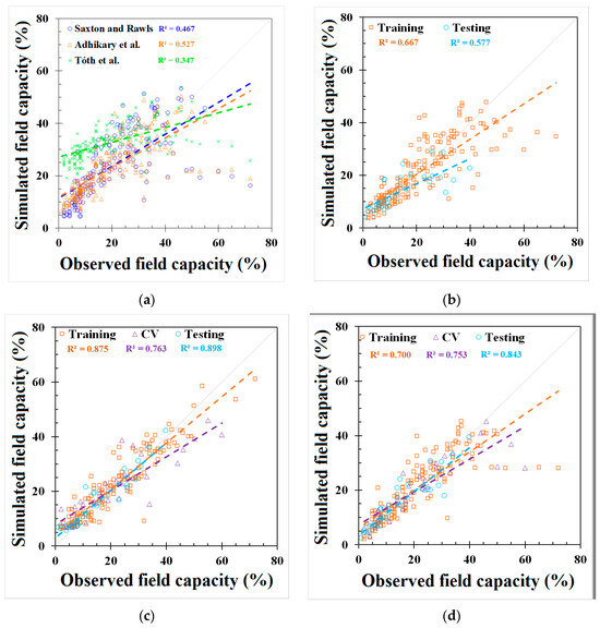
Figure 2.
Modeling results of field capacity (FC) from (a) Saxton and Rawls, Adhikary et al., and Tóth et al. models, (b) REG model, (c) ANN model, and (d) GEP model.
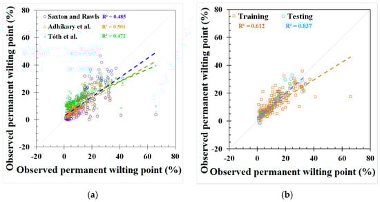
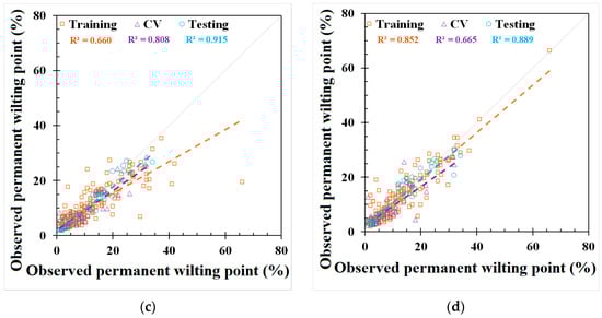
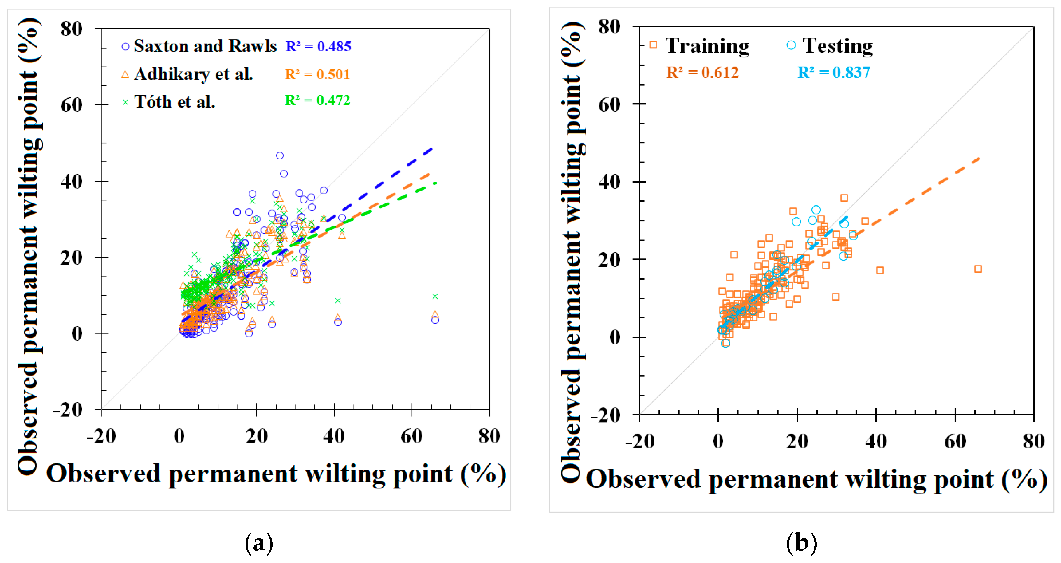
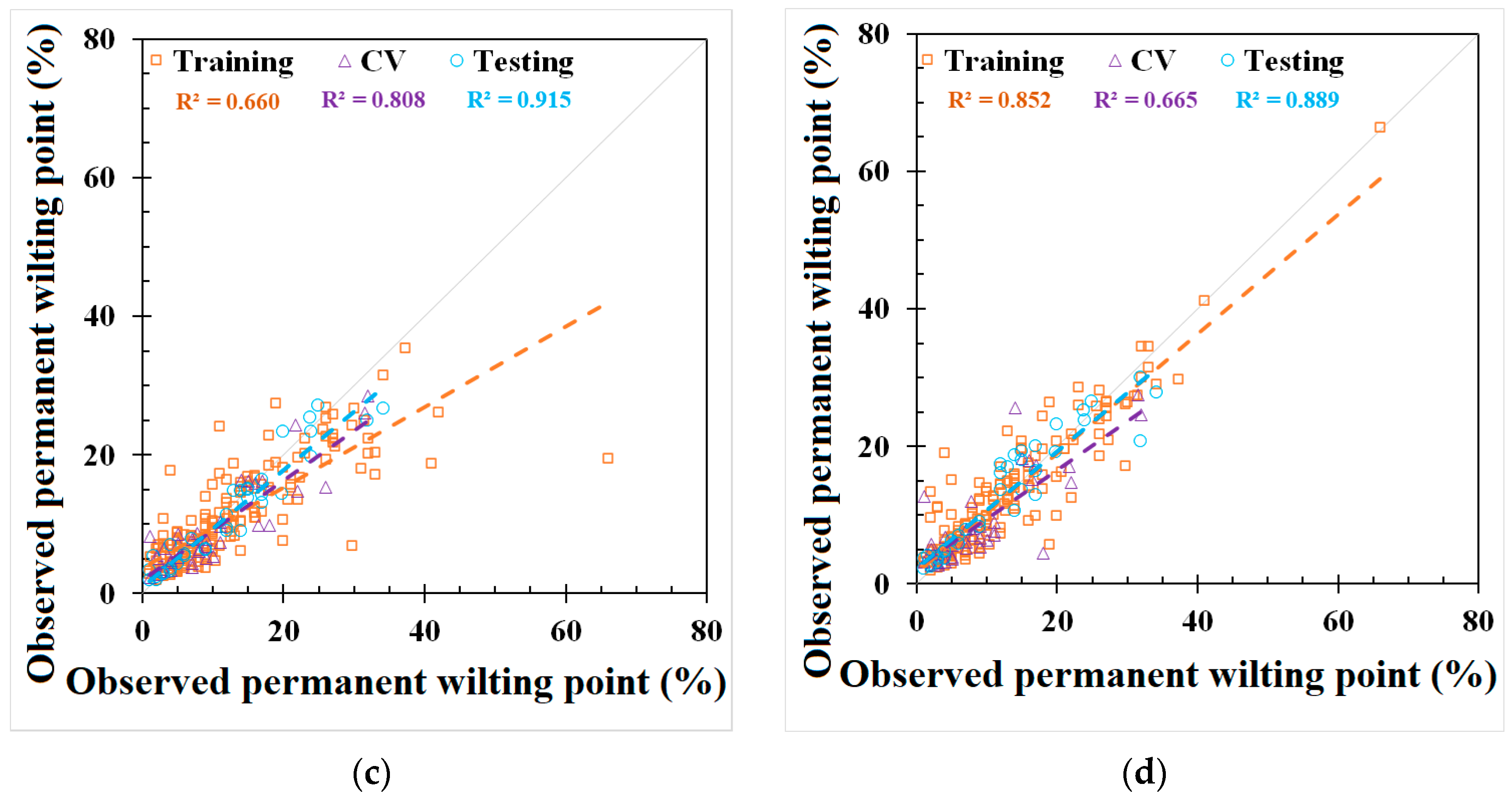
Figure 3.
Modeling results of permanent wilting point (PWP) from (a) Saxton and Rawls, Adhikary et al., and Tóth et al. models, (b) REG model, (c) ANN model, and (d) GEP model.
Table 3.
Model input and performance parameters on the testing dataset.
The simulation results for the different models in predicting the FC and PWP are summarized with their respective NRMSE values. For FC prediction, the models exhibited varying degrees of accuracy. According to the classification criteria adapted from Jamieson et al. [47], the GEP model, with an NRMSE of 29.9%, performed the best among all models and was classified as fair. The ANN model, with an NRMSE of 31.9%, was slightly higher but still falls into the poor category. Other models such as the REG, the model by Adhikary et al., and the model by Saxton and Rawls had NRMSE values of 49.2%, 52.2%, and 56.3%, respectively, and were all categorized as poor. Tóth et al. had the highest NRMSE at 123.9%, highlighting that the existing FC models may produce significant errors when using global scale datasets. For PWP prediction, the ANN model outperformed other models significantly, with an NRMSE of 19.9%, classifying it as good. The GEP model followed with an NRMSE of 22.3%, which is considered fair. Tóth et al. showed an NRMSE of 37.7%, falling into the poor category. The Saxton and Rawls, Adhikary et al., and REG models had NRMSE values of 41.6%, 62.2%, and 69.0%, respectively, and were all classified as poor. The NRMSE evaluation on the FC and PWP indicates that the ML-based algorithms provide a relatively accurate prediction.
where FCREG is the field capacity and PWPREG is the permanent wilting point in the REG model (%); Lo is the longitude; La is the latitude; Al is the altitude (m); Sa is the sand content (%); Si is the silt content (%); C is the clay content (%); and EC is the electrical conductivity (ds/m). In the ANN model, due to the complex connections between neurons at different layers, a mathematical formula cannot be derived.
3.3. Identification of Dominant Input Variables
In order to determine the relative importance of the input variables included in the best-fit combinations of variables, K-S analysis was conducted and the results for altitude, sand, silt, clay, EC, and pH, are shown in Table 4. The results showed that clay, sand, and silt in the FC model and altitude and EC in the PWP model have significant impacts on preventing higher absolute errors in FC and PWP simulation. Longitude and latitude were not included in the K-S analysis due to the wide range of values for these two parameters in the database. However, it is clear that geographical locations play essential roles in FC and PWP modeling, which agrees with the conclusions of [9,13,23]. Despite the fact that pH and EC do not always decrease the error in FC and PWP modeling, the inclusion of these two parameters in the combination of input variables generally improves the model’s performance.
Table 4.
Significance analysis by Kolmogorov–Smirnov test.
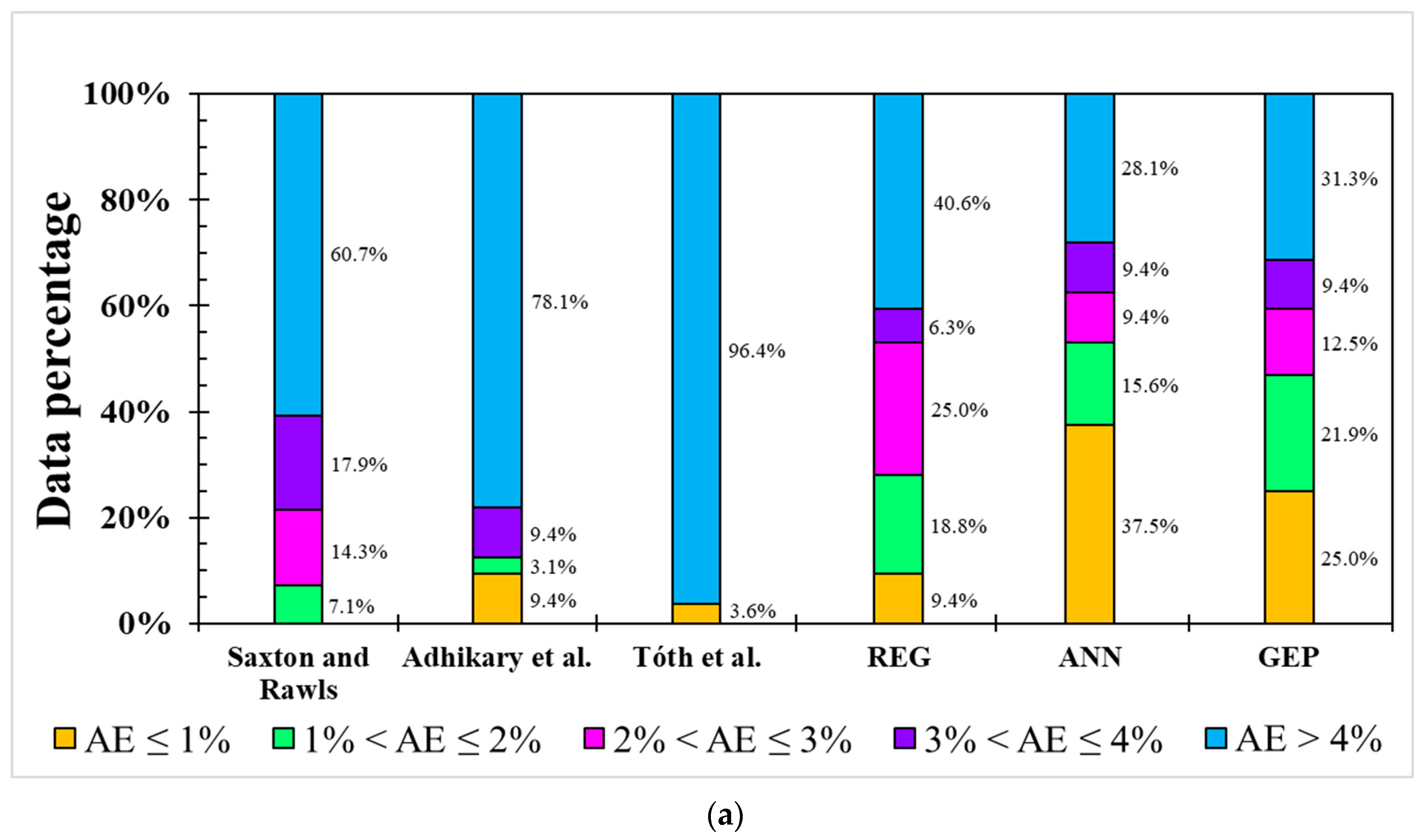
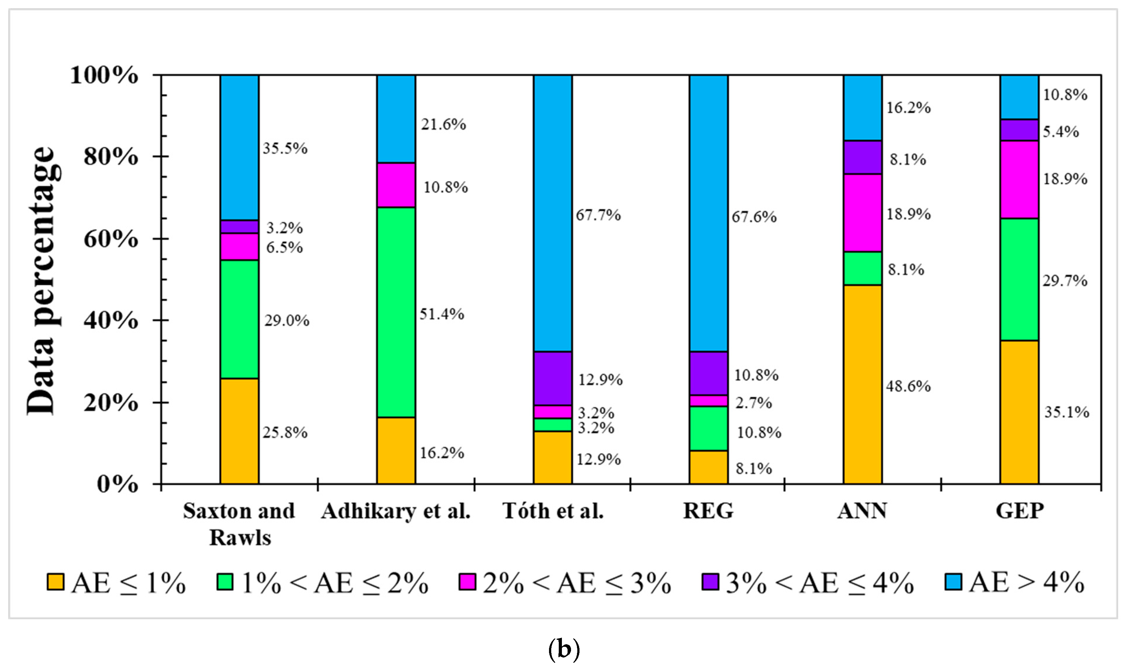
For the model error distribution analysis, the comprehensive modeling capacity of each model was evaluated by above-mentioned indicators. However, R2 only describes the model’s responded variation between dependent variables and independent variables. RMSE, NRMSE, and MAE are averaged errors that cannot represent the error distribution, i.e., indicating the primary range of the error. In order to evaluate each model’s error distribution, the absolute error (AE) was utilized in the testing dataset of each model for both the FC and PWP (Figure 4). Five categories were used, including AE ≤ 1, 1 < AE ≤ 2, 2 < AE ≤ 3, 3 < AE ≤ 4, and AE > 4. Figure 4a shows the AE distribution in the FC model. All linear-based models have lower accuracy (AE ≤ 1%), ranging from 0% to 9.4%, and an unignored error (AE > 4%) from 40.6% to 96.4%. In contrast, ML-based ANN and GEP models demonstrate better simulation ability (AE ≤ 1%) from 25.0% to 37.5% and the massive error (>4%) is from 28.1% to 31.3%. Over 60% of AEs in the three PTFs in previous studies are greater than 4% although the FC modeling result from the study of Adhikary et al. [36] presented an acceptable R2 (0.683), but around 78.1% of AEs were higher than 4%.
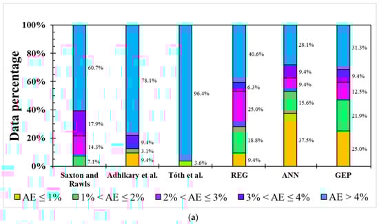

Figure 4.
Occurrence of absolute error (AE) from different models for (a) FC and (b) PWP simulation.
The result for the PWP simulation was similar to the ANN and GEP models and had greater modeling ability than linear-based models in terms of AE distribution, as shown in Figure 4b. Notably, the GEP model showed a higher simulation ability to avoid large errors (AE > 4%) than the ANN model, almost 90% of AEs in the GEP model were lower than 4% while this value was only 84% in the ANN model. It should be mentioned that the model applied by Adhikary et al. [36] only used sand and silt in modeling the FC and clay in modeling the PWP, meaning that this model has the lowest dataset requirement. In situations in which resources to analyze OM, pH, and EC are not available, equations from Adhikary et al. [36] can be used to provide rough estimations of the FC and PWP values. When EC and pH data are available, the ML-based ANN model is an effective and more accurate algorithm to predict the FC and PWP. However, the ANN model requires more sophisticated hardware support and knowledge than the GEP model. Therefore, considering the applicability and performance, GEP has some advantages over ANN for the FC and PWP simulation.
4. Conclusions
The Field capacity (FC) and permanent wilting point (PWP) are critical metrics in soil health assessment. Yet, direct measurement of their values is often challenging. In the study, data from the World Soil Information Service (WoSIS) were utilized, and advanced algorithms, specifically the artificial neural network (ANN) and gene-expression programming (GEP) algorithms, were employed to predict the FC and PWP using accessible parameters. Optimal variables for modeling the FC and PWP were identified including longitude; latitude; altitude; sand, silt, and clay content; electrical conductivity; and pH. Significantly, the ML-based ANN and GEP models achieved higher modeling accuracy, compared with the conventional, linear-based FC and PWP model developed in Adhikary et al. [36].
The NRMSE evaluation showed that the ANN model was best for PWP prediction, while the GEP model performed best for FC prediction, both providing relatively accurate results. Although greater model interpretability was exhibited by the ANN, greater resilience against substantial errors was demonstrated by the GEP model. However, it is important to note that caution must be exercised when applying these models to current soils because while soil changes are minimal when undisturbed or undeveloped, the collection times for data in the WoSIS database vary. This might result in disparities between the database’s information and the current state of soil development.
Overall, this study revealed that machine learning, particularly in the GEP model, can be effectively used to predict the FC and PWP using WoSIS data. These results can be used to improve rational irrigation practices, akin to IoT-based smart irrigation systems as reported by [54]. This enhanced irrigation scheme could lower water consumption in agriculture, reduce the likelihood of crop failures, and potentially decrease greenhouse gas emissions, marking a significant advancement in soil health evaluation and environmental stewardship. Future studies are encouraged to explore a broader range of machine learning models and to refine predictive accuracy further, thereby enhancing the management of soil resources and the resilience of agricultural ecosystems.
Author Contributions
Conceptualization, L.L. and X.M.; methodology, L.L.; software, L.L.; validation, L.L. and X.M.; formal analysis, L.L.; resources, L.L. and X.M.; data curation, L.L.; writing—original draft preparation, L.L.; writing—review and editing, X.M.; visualization, L.L. and X.M.; supervision, X.M.; funding acquisition, L.L. and X.M. All authors have read and agreed to the published version of the manuscript.
Funding
This work is partially supported by the USDA National Institute of Food and Agriculture, AFRI project (2023-67021-39755), the Ministry of Science and Technology, Taiwan (109-2917-I-020-001), and the National Science and Technology Council, Taiwan (113-2221-E-020-009-MY3).
Data Availability Statement
The data used in this study can be found in the following references: [32]. Batjes, N. H., Ribeiro, E., & Van Oostrum, A. (2020). Standardised soil profile data to support global mapping and modelling (WoSIS snapshot 2019). Earth System Science Data, 12(1), 299-320. [34]. Ribeiro, E., Batjes, N. H., & Van Oostrum, A. J. M. (2018). World Soil Information Service (WoSIS)-Towards the standardization and harmonization of world soil data. Procedures manual, 166.
Acknowledgments
The authors gratefully acknowledge the Department of Civil and Environmental Engineering, Texas A&M University for providing computing equipment and the Taiwan government for research funding.
Conflicts of Interest
The authors declare no conflicts of interest.
Abbreviations
| Abbreviation | Meaning |
| AE | absolute error |
| Al | altitude |
| ANN | artificial neural network |
| BPNN | backpropagation neural network |
| CEC | cation exchange capacity |
| C | clay content |
| CV | cross-validation |
| DL | deep learning |
| EC | electrical conductivity |
| FC | field capacity |
| FCANN | field capacity in ANN model |
| FCGEP | field capacity in GEP model |
| FCREG | field capacity in REG model |
| GA | gene algorithm |
| GEP | gene expression programming |
| GP | gene programming |
| i | datum order |
| k-NN | k-nearest neighbors |
| K-S test | Kolmogorov–Smirnov nonparametric test |
| La | latitude |
| Lo | longitude |
| MAE | mean absolute error |
| Max. | maximum |
| Min. | minimum |
| ML | machine learning |
| n | number of actual observations |
| NF | neuro-fuzzy |
| NRMSE | normalized root mean square error |
| OM | organic matter |
| PTF | pedotransfer functions |
| PWP | permanent wilting point |
| PWPANN | permanent wilting point in ANN model |
| PWPGEP | permanent wilting point in GEP model |
| PWPREG | permanent wilting point in REG model |
| r | correlation coefficient |
| REG | regression |
| RF | random forest |
| RMSE | root mean square error |
| R2 | coefficient of determination |
| RT | regression trees |
| S | soil textures (sand, silt, and clay content) |
| Sa | sand content |
| Si | silt content |
| SOM | soil organic matter |
| SVM | support vector machine |
| SWC | soil water content |
| WoSIS | World Soil Information Service |
| x | observed value |
| xmax | maximum observed value |
| xmin | minimum observed value |
| xnorm | normalized dimensionless variable |
| observed value in ith datum | |
| predicted value in ith datum | |
| average of the observations | |
| μ | average |
| σ | standard deviation |
| α | slope of the linear equation |
| β | intercept of the regression |
| ε | error term |
Appendix A. Soil Group and Nations of the FC and PWP Model
In total, 20 countries with 24 Food and Agriculture Organization (FAO) soil groups for field capacity (FC) model development and 27 countries with 25 FAO soil groups for permanent wilting point (PWP) model establishment (Table A1).
Table A1.
FAO soil group and observed country in FC and PWP model.
Table A1.
FAO soil group and observed country in FC and PWP model.
| Country | Target | Acrisols | Andosols | Arenosols | Calcisols | Cambisols | Chernozems | Ferralsols | Fluvisols | Kastanozems | Leptosols | Lixisols | Luvisols |
|---|---|---|---|---|---|---|---|---|---|---|---|---|---|
| Albania | FC | 2 | |||||||||||
| PWP | 2 | ||||||||||||
| Benin | FC | ||||||||||||
| PWP | 1 | ||||||||||||
| Burkina Faso | FC | 2 | |||||||||||
| PWP | 2 | ||||||||||||
| Canada | FC | 1 | 2 | ||||||||||
| PWP | 1 | 2 | 1 | 2 | |||||||||
| Colombia | FC | 5 | |||||||||||
| PWP | 5 | ||||||||||||
| Ecuador | FC | ||||||||||||
| PWP | 1 | ||||||||||||
| Ethiopia | FC | ||||||||||||
| PWP | |||||||||||||
| Germany | FC | 10 | 1 | 5 | 1 | ||||||||
| PWP | 10 | 1 | 5 | 1 | |||||||||
| India | FC | 4 | |||||||||||
| PWP | 4 | ||||||||||||
| Indonesia | FC | 6 | |||||||||||
| PWP | 6 | 1 | |||||||||||
| Jamaica | FC | ||||||||||||
| PWP | 1 | ||||||||||||
| Jordan | FC | 1 | |||||||||||
| PWP | 1 | ||||||||||||
| Kenya | FC | 1 | 2 | ||||||||||
| PWP | 1 | 2 | |||||||||||
| Mozambique | FC | 1 | 1 | 1 | 1 | ||||||||
| PWP | 1 | 1 | 1 | 1 | |||||||||
| Poland | FC | ||||||||||||
| PWP | |||||||||||||
| Portugal | FC | 2 | 2 | 1 | |||||||||
| PWP | 2 | 2 | 1 | ||||||||||
| Puerto Rico | FC | ||||||||||||
| PWP | 1 | ||||||||||||
| Sierra Leone | FC | 1 | |||||||||||
| PWP | 1 | ||||||||||||
| South Africa | FC | 15 | 15 | 1 | 9 | 2 | 1 | 1 | 1 | 18 | 22 | ||
| PWP | 15 | 15 | 1 | 9 | 2 | 1 | 1 | 1 | 18 | 22 | |||
| Suriname | FC | ||||||||||||
| PWP | 2 | 9 | |||||||||||
| Sweden | FC | ||||||||||||
| PWP | |||||||||||||
| Thailand | FC | 1 | |||||||||||
| PWP | 1 | ||||||||||||
| UK | FC | ||||||||||||
| PWP | 1 | ||||||||||||
| Tanzania | FC | 1 | 2 | ||||||||||
| PWP | 1 | 2 | |||||||||||
| USA | FC | ||||||||||||
| PWP | |||||||||||||
| Zambia | FC | 4 | |||||||||||
| PWP | 4 | ||||||||||||
| Zimbabwe | FC | 2 | |||||||||||
| PWP | 2 | ||||||||||||
| Uncategorized | FC | 4 | |||||||||||
| PWP | 21 |
Table A2.
FAO soil group and observed country in FC and PWP model continued.
Table A2.
FAO soil group and observed country in FC and PWP model continued.
| Country | Target | Nitisols | Nitosols | Phaeozems | Planosols | Plinthosols | Podzols | Podzoluvisols | Regosols | Rendzinas | Solonetz | Vertisols | Xerosols | Yermosols |
|---|---|---|---|---|---|---|---|---|---|---|---|---|---|---|
| Albania | FC | 1 | 1 | |||||||||||
| PWP | 1 | 1 | ||||||||||||
| Benin | FC | |||||||||||||
| PWP | ||||||||||||||
| Burkina Faso | FC | |||||||||||||
| PWP | ||||||||||||||
| Canada | FC | |||||||||||||
| PWP | ||||||||||||||
| Colombia | FC | |||||||||||||
| PWP | ||||||||||||||
| Ecuador | FC | |||||||||||||
| PWP | ||||||||||||||
| Ethiopia | FC | 2 | ||||||||||||
| PWP | 2 | |||||||||||||
| Germany | FC | 3 | ||||||||||||
| PWP | 3 | |||||||||||||
| India | FC | 4 | 4 | 1 | ||||||||||
| PWP | 4 | 4 | 1 | |||||||||||
| Indonesia | FC | |||||||||||||
| PWP | ||||||||||||||
| Jamaica | FC | |||||||||||||
| PWP | ||||||||||||||
| Jordan | FC | 2 | 1 | |||||||||||
| PWP | 2 | 1 | ||||||||||||
| Kenya | FC | |||||||||||||
| PWP | ||||||||||||||
| Mozambique | FC | |||||||||||||
| PWP | ||||||||||||||
| Poland | FC | |||||||||||||
| PWP | 1 | |||||||||||||
| Portugal | FC | |||||||||||||
| PWP | ||||||||||||||
| Puerto Rico | FC | |||||||||||||
| PWP | ||||||||||||||
| Sierra Leone | FC | |||||||||||||
| PWP | ||||||||||||||
| South Africa | FC | 6 | 1 | 7 | 2 | 9 | 6 | 2 | ||||||
| PWP | 6 | 1 | 7 | 2 | 9 | 6 | 2 | |||||||
| Suriname | FC | |||||||||||||
| PWP | 5 | |||||||||||||
| Sweden | FC | 1 | ||||||||||||
| PWP | 1 | |||||||||||||
| Thailand | FC | |||||||||||||
| PWP | ||||||||||||||
| UK | FC | |||||||||||||
| PWP | ||||||||||||||
| Tanzania | FC | 1 | ||||||||||||
| PWP | 1 | |||||||||||||
| USA | FC | 3 | ||||||||||||
| PWP | 4 | |||||||||||||
| Zambia | FC | 1 | ||||||||||||
| PWP | 1 | |||||||||||||
| Zimbabwe | FC | |||||||||||||
| PWP |

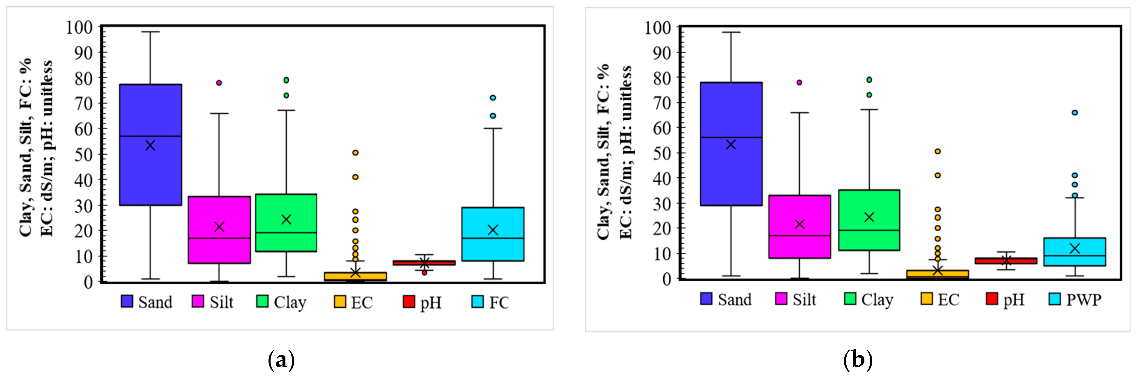
Figure A1.
Modeling dataset boxplot of (a) the FC and (b) the PWP. The top and bottom lines are the maximum and minimum observation above/below the fence (1.5 × interquartile range), respectively. The upper and lower boundaries of the box are the 75th and 25th percentage data, respectively. The cross-mark and line in the box are the mean and median of the dataset.
Appendix B. Used Parameters of Each Factor of Published PTFs
Table A3.
Used parameters of each factor of published PTFs.
Table A3.
Used parameters of each factor of published PTFs.
| PTFs | Target | Soil | Silt | Clay | Organic Matters | Sa × OM | C × OM | Sa × C | Si × C | 1/(OM + 1) | Si × OM’ | C × OM’ | Constant |
|---|---|---|---|---|---|---|---|---|---|---|---|---|---|
| Sa | Si | C | OM | OM’ | |||||||||
| Saxton and Rawls | FC’ | −0.251 | 0.195 | 0.011 | 0.006 | −0.027 | 0.452 | 0.299 | |||||
| FC | FC’ + (1.283(FC’)2 − 0.374(FC’) − 0.015) | ||||||||||||
| Adhikary et al. | FC | −0.51 | −0.27 | 56.37 | |||||||||
| Tóth et al. | FC | 0.00154 | 0.00453 | −0.000511 | −0.1887 | 0.00144 | 0.00087 | 0.2449 | |||||
| Saxton and Rawls | PWP’ | −0.024 | 0.487 | 0.006 | 0.005 | −0.013 | 0.068 | 0.031 | |||||
| PWP | PWP’ + (0.14(PWP’) − 0.02) | ||||||||||||
| Adhikary et al. | PWP | 0.44000 | 0.71 | ||||||||||
| Tóth et al. | PWP | −0.00084 | 0.00213 | 0.000385 | −0.0767 | 0.00095 | 0.00233 | 0.09878 | |||||
Appendix C. Model Performance and Comparisons
Table A4.
Model performance of published PTFs, ANN, GEP, and REG.
Table A4.
Model performance of published PTFs, ANN, GEP, and REG.
| Target | Model | Data | R2 | RMSE | NRMSE | MAE | ||||||||||
|---|---|---|---|---|---|---|---|---|---|---|---|---|---|---|---|---|
| Training | CV | Testing | Training | CV | Testing | Training | CV | Testing | Training | CV | Testing | Training | CV | Testing | ||
| FC | Saxton and Rawls | Total: 179 | Total: 0.467 | Total: 11.254 | Total: 55.6% | Total: 8.120 | ||||||||||
| Adhikary et al. | Total: 210 | Total: 0.527 | Total: 9.969 | Total: 49.2% | Total: 7.369 | |||||||||||
| Tóth et al. | Total: 179 | Total: 0.347 | Total: 17.225 | Total: 85.0% | Total: 15.575 | |||||||||||
| REG | 178 | - | 32 | 0.667 | - | 0.577 | 8.200 | - | 7.053 | 38.5% | - | 49.2% | 5.438 | - | 5.005 | |
| ANN | 146 | 32 | 32 | 0.875 | 0.763 | 0.898 | 4.910 | 8.013 | 4.574 | 23.2% | 36.3% | 31.9% | 3.683 | 6.022 | 3.133 | |
| GEP | 146 | 32 | 32 | 0.700 | 0.753 | 0.843 | 7.487 | 8.337 | 4.290 | 35.4% | 37.7% | 29.9% | 4.628 | 4.672 | 3.115 | |
| PWP | Saxton and Rawls | Total: 221 | Total: 0.485 | Total: 18.918 | Total: 157.5% | Total: 14.392 | ||||||||||
| Adhikary et al. | Total: 254 | Total: 0.501 | Total: 17.699 | Total: 147.3% | Total: 13.494 | |||||||||||
| Tóth et al. | Total: 221 | Total: 0.472 | Total: 16.244 | Total: 135.2% | Total: 12.705 | |||||||||||
| REG | 217 | - | 37 | 0.612 | - | 0.837 | 5.836 | - | 8.475 | 49.8% | - | 69.0% | 3.531 | - | 6.122 | |
| ANN | 180 | 37 | 37 | 0.660 | 0.808 | 0.915 | 6.031 | 3.774 | 2.442 | 49.1% | 36.9% | 19.9% | 3.514 | 2.778 | 1.758 | |
| GEP | 180 | 37 | 37 | 0.852 | 0.665 | 0.889 | 3.723 | 4.551 | 2.746 | 30.8% | 46.5% | 22.3% | 2.542 | 3.083 | 2.000 | |
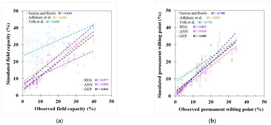
Figure A2.
Model testing dataset comparison in (a) FC and (b) PWP.
Figure A2.
Model testing dataset comparison in (a) FC and (b) PWP.
Appendix D. Python-Based FCGEP and PWPGEP Models
- Python-based FCGEP model
- # This model was implemented using Python 3.8. Ensure compatibility with this version.
- # Considering potential future updates to Python that may lead to compatibility issues with certain modules, the authors recommend that future users assess compatibility with the following sections when using different versions of Python.
- From math import *
- def fieldCapacity(d):
C1 = −21.2657870372787; C2 = −9.7779381694998; C3 = 4.57090956378595;
C4 = 1.06872399344557;
latitude = 0; longitude = 1; altitude = 2; EC = 3; clay = 4; sand = 5;
silt = 6
y = 0.0
y = (((d[clay]+(1.0/((d[latitude]/C1))))/2.0)+((((((d[latitude]+d[sand]+d[sand]+d[silt])/4.0)+min(d[silt],d[sand],d[sand])+d[silt]+d[latitude])/4.0)+cos(d[altitude]))/2.0))
y = min(y,(((tan((d[EC]+d[longitude]))+(((d[EC]*d[EC]*d[silt])+((d[silt]+d[clay]+C3 +C4)/4.0)+d[latitude]+d[silt])/4.0))/2.0)+((d[clay]+((C2+d[altitude])/2.0))/2.0)))
return y
- 2.
- Python-based PWPGEP model
- # This model was implemented using Python 3.8. Ensure compatibility with this version.
- # Considering potential future updates to Python that may lead to compatibility issues with certain modules, the authors recommend that future users assess compatibility with the following sections when using different versions of Python.
- From math import *
- def permanentWiltingPoint(d):
C1 = −4.9227785356074; C2 = −8.26012200863814; C3 = −5.76989349040193;
C4 = −0.9464415417951; C5 = −3.81722107697073; C6 = −6.20128482924894;
C7 = −8.31278145411878
latitude = 0; longitude = 1; altitude = 2; EC = 3; pH = 4; clay = 5; sand = 6; silt = 7
y = 0.0
y = atan(gep3Rt(floor(pow(pow(pow(gep3Rt(d[sand]),(1.0/4.0)),5.0),floor(atan(log(d[pH])))))))
y = y * (d[clay]-gep3Rt((min((C1*d[latitude]),(d[clay]+d[clay]+d[pH]+C1))-((d[silt]+d[sand])/2.0)-tan(d[latitude])-d[latitude])))
y = y * asin((atan((1.0/((C2+((((d[silt]+d[latitude]+d[longitude]+C4)/4.0))/((d[altitude]+C3+d[altitude]+d[clay])/4.0))))))))
y = y * min(C5,((((d[sand]-d[EC]-C5-d[altitude])+(d[longitude]-C6))+tan((d[longitude]-C7))+pow((d[altitude]-d[sand]),2.0))/3.0))
y = y * pow(sin(gep5Rt(d[pH])),5.0)
return y
def gep3Rt(x):
if (x < 0.0):
return −pow(−x,(1.0/3.0))
else:
return pow(x,(1.0/3.0))
- def gep5Rt(x):
if (x < 0.0):
return −pow(−x,(1.0/5.0))
else:
return pow(x,(1.0/5.0))
References
- Brady, N.C.; Weil, R.R.; Weil, R.R. The Nature and Properties of Soils; Prentice Hall: Upper Saddle River, NJ, USA, 2008; Volume 13. [Google Scholar]
- Assi, A.T.; Blake, J.; Mohtar, R.H.; Braudeau, E. Soil aggregates structure-based approach for quantifying the field capacity, permanent wilting point and available water capacity. Irrig. Sci. 2019, 37, 511–522. [Google Scholar] [CrossRef]
- Hoogenboom, G.; Porter, C.; Shelia, V.; Boote, K.; Singh, U.; White, J.; Hunt, L.; Ogoshi, R.; Lizaso, J.; Koo, J. Decision Support System for Agrotechnology Transfer (DSSAT); Version 4.7; DSSAT Foundation: Gainesville, FL, USA, 2017; Available online: https://DSSAT.net (accessed on 1 March 2023).
- Pentoś, K.; Pieczarka, K.; Serwata, K. The Relationship between Soil Electrical Parameters and Compaction of Sandy Clay Loam Soil. Agriculture 2021, 11, 114. [Google Scholar] [CrossRef]
- Mohanty, B.; Gaur, N. Near Surface Soil Moisture Controls Beyond the Darcy Support Scale: A Remote Sensing Perspective. In Proceedings of the AGU Fall Meeting Abstracts, San Francisco, CA, USA, 15–19 December 2014; p. H13D-1135. [Google Scholar]
- Tunçay, T.; Başkan, O.; Bayramın, I.; Dengız, O.; Kılıç, Ş. Geostatistical approach as a tool for estimation of field capacity and permanent wilting point in semi-arid terrestrial ecosystem. Arch. Agron. Soil Sci. 2018, 64, 1240–1253. [Google Scholar] [CrossRef]
- Jian, J.; Du, X.; Stewart, R.D. A database for global soil health assessment. Sci. Data 2020, 7, 16. [Google Scholar] [CrossRef]
- McBratney, A.B.; Santos, M.M.; Minasny, B. On digital soil mapping. Geoderma 2003, 117, 3–52. [Google Scholar] [CrossRef]
- Santra, P.; Kumar, M.; Kumawat, R.; Painuli, D.; Hati, K.; Heuvelink, G.; Batjes, N. Pedotransfer functions to estimate soil water content at field capacity and permanent wilting point in hot Arid Western India. J. Earth Syst. Sci. 2018, 127, 35. [Google Scholar] [CrossRef]
- Morgan, C.L. Assessing Soil Health: Soil Water Cycling. Crops Soils 2020, 53, 35–41. [Google Scholar] [CrossRef]
- Nourbakhsh, F.; Afyuni, M.; Abbaspour, K.C.; Schulin, R. Research note: Estimation of field capacity and wilting point from basic soil physical and chemical properties. Arid Land Res. Manag. 2004, 19, 81–85. [Google Scholar] [CrossRef]
- Taşan, S.; Demir, Y. Comparative Analysis of MLR, ANN, and ANFIS Models for Prediction of Field Capacity and Permanent Wilting Point for Bafra Plain Soils. Commun. Soil Sci. Plant Anal. 2020, 51, 604–621. [Google Scholar] [CrossRef]
- Jin, X.; Wang, S.; Yu, N.; Zou, H.; An, J.; Zhang, Y.; Wang, J.; Zhang, Y. Spatial predictions of the permanent wilting point in arid and semi-arid regions of Northeast China. J. Hydrol. 2018, 564, 367–375. [Google Scholar] [CrossRef]
- Cueff, S.; Coquet, Y.; Aubertot, J.-N.; Bel, L.; Pot, V.; Alletto, L. Estimation of soil water retention in conservation agriculture using published and new pedotransfer functions. Soil Tillage Res. 2021, 209, 104967. [Google Scholar] [CrossRef]
- Rotnitzky, A.; Wypij, D. A note on the bias of estimators with missing data. Biometrics 1994, 50, 1163–1170. [Google Scholar] [CrossRef]
- Tóth, B.; Weynants, M.; Nemes, A.; Makó, A.; Bilas, G.; Tóth, G. New generation of hydraulic pedotransfer functions for Europe. Eur. J. Soil Sci. 2015, 66, 226–238. [Google Scholar] [CrossRef]
- Tunçay, T.; Kılıç, Ş.; Dedeoğlu, M.; Dengiz, O.; Başkan, O.; Bayramin, İ. Assessing soil fertility index based on remote sensing and gis techniques with field validation in a semiarid agricultural ecosystem. J. Arid Environ. 2021, 190, 104525. [Google Scholar] [CrossRef]
- Keshavarzi, R.; Mohammadi, S. A new approach for numerical modeling of hydraulic fracture propagation in naturally fractured reservoirs. In Proceedings of the SPE/EAGE European Unconventional Resources Conference and Exhibition—From Potential to Production, Vienna, Austria, 20–22 March 2012; p. cp-285-00039. [Google Scholar]
- Mohanty, M.; Sinha, N.K.; Painuli, D.; Bandyopadhyay, K.; Hati, K.; Reddy, K.S.; Chaudhary, R. Modelling soil water contents at field capacity and permanent wilting point using artificial neural network for Indian soils. Natl. Acad. Sci. Lett. 2015, 38, 373–377. [Google Scholar] [CrossRef]
- Shiri, J.; Keshavarzi, A.; Kisi, O.; Karimi, S. Using soil easily measured parameters for estimating soil water capacity: Soft computing approaches. Comput. Electron. Agric. 2017, 141, 327–339. [Google Scholar] [CrossRef]
- Gunarathna, M.; Sakai, K.; Nakandakari, T.; Momii, K.; Kumari, M.; Amarasekara, M. Pedotransfer functions to estimate hydraulic properties of tropical Sri Lankan soils. Soil Tillage Res. 2019, 190, 109–119. [Google Scholar] [CrossRef]
- Ghorbani, M.A.; Shamshirband, S.; Haghi, D.Z.; Azani, A.; Bonakdari, H.; Ebtehaj, I. Application of firefly algorithm-based support vector machines for prediction of field capacity and permanent wilting point. Soil Tillage Res. 2017, 172, 32–38. [Google Scholar] [CrossRef]
- Yamaç, S.S.; Şeker, C.; Negiş, H. Evaluation of machine learning methods to predict soil moisture constants with different combinations of soil input data for calcareous soils in a semi arid area. Agric. Water Manag. 2020, 234, 106121. [Google Scholar] [CrossRef]
- Hateffard, F.; Dolati, P.; Heidari, A.; Zolfaghari, A.A. Assessing the performance of decision tree and neural network models in mapping soil properties. J. Mt. Sci. 2019, 16, 1833–1847. [Google Scholar] [CrossRef]
- McCutcheon, M.; Farahani, H.; Stednick, J.; Buchleiter, G.; Green, T. Effect of soil water on apparent soil electrical conductivity and texture relationships in a dryland field. Biosyst. Eng. 2006, 94, 19–32. [Google Scholar] [CrossRef]
- Frost, P.S.; van Es, H.M.; Rossiter, D.G.; Hobbs, P.R.; Pingali, P.L. Soil health characterization in smallholder agricultural catchments in India. Appl. Soil Ecol. 2019, 138, 171–180. [Google Scholar] [CrossRef]
- Corwin, D.L.; Lesch, S.M. Apparent soil electrical conductivity measurements in agriculture. Comput. Electron. Agric. 2005, 46, 11–43. [Google Scholar] [CrossRef]
- Allen, D.E.; Singh, B.P.; Dalal, R.C. Soil health indicators under climate change: A review of current knowledge. In Soil Health and Climate Change; Springer: Berlin/Heidelberg, Germany, 2011; pp. 25–45. [Google Scholar]
- Sinha, S.K.; Wang, M.C. Artificial Neural Network Prediction Models for Soil Compaction and Permeability. Geotech. Geol. Eng. 2008, 26, 47–64. [Google Scholar] [CrossRef]
- Besalatpour, A.; Hajabbasi, M.; Ayoubi, S.; Afyuni, M.; Jalalian, A.; Schulin, R. Soil shear strength prediction using intelligent systems: Artificial neural networks and an adaptive neuro-fuzzy inference system. Soil Sci. Plant Nutr. 2012, 58, 149–160. [Google Scholar] [CrossRef]
- Pham, V.-N.; Oh, E.; Ong, D.E.L. Effects of binder types and other significant variables on the unconfined compressive strength of chemical-stabilized clayey soil using gene-expression programming. Neural Comput. Appl. 2022, 34, 9103–9121. [Google Scholar] [CrossRef]
- Batjes, N.H.; Ribeiro, E.; van Oostrum, A. Standardised soil profile data to support global mapping and modelling (WoSIS snapshot 2019). Earth Syst. Sci. Data 2020, 12, 299–320. [Google Scholar] [CrossRef]
- Batjes, N.H.; Ribeiro, E.; van Oostrum, A.; Leenaars, J.; Hengl, T.; Mendes de Jesus, J. WoSIS: Providing standardised soil profile data for the world. Earth Syst. Sci. Data 2017, 9, 1–14. [Google Scholar] [CrossRef]
- Ribeiro, E.; Batjes, N.; Van Oostrum, A.J.M. World Soil Information Service (WoSIS)—Towards the Standardization and Harmonization of World Soil Data; ISRIC, World Soil Information: Wageningen, The Netherlands, 2018; Volume 166. [Google Scholar]
- Saxton, K.E.; Rawls, W.J. Soil water characteristic estimates by texture and organic matter for hydrologic solutions. Soil Sci. Soc. Am. J. 2006, 70, 1569–1578. [Google Scholar] [CrossRef]
- Adhikary, P.P.; Chakraborty, D.; Kalra, N.; Sachdev, C.; Patra, A.; Kumar, S.; Tomar, R.; Chandna, P.; Raghav, D.; Agrawal, K. Pedotransfer functions for predicting the hydraulic properties of Indian soils. Soil Res. 2008, 46, 476–484. [Google Scholar] [CrossRef]
- Liu, L.-W.; Hsieh, S.-H.; Lin, S.-J.; Wang, Y.-M.; Lin, W.-S. Rice Blast (Magnaporthe oryzae) Occurrence Prediction and the Key Factor Sensitivity Analysis by Machine Learning. Agronomy 2021, 11, 771. [Google Scholar] [CrossRef]
- Hsieh, S.-H.; Liu, L.-W.; Chung, W.-G.; Wang, Y.-M. Sensitivity analysis on the rising relation between short-term rainfall and groundwater table adjacent to an artificial recharge lake. Water 2019, 11, 1704. [Google Scholar] [CrossRef]
- Ferreira, C. Gene expression programming in problem solving. In Soft Computing and Industry; Springer: London, UK, 2002; pp. 635–653. [Google Scholar]
- Liu, L.-W.; Wang, Y.-M. Modelling reservoir turbidity using Landsat 8 satellite imagery by gene expression programming. Water 2019, 11, 1479. [Google Scholar] [CrossRef]
- Wang, X.; Liu, L.; Zhang, W.; Ma, X. Prediction of Plant Uptake and Translocation of Engineered Metallic Nanoparticles by Machine Learning. Environ. Sci. Technol. 2021, 55, 7491–7500. [Google Scholar] [CrossRef]
- Lee, C.-H.; Liu, L.-W.; Wang, Y.-M.; Leu, J.-M.; Chen, C.-L. Drone-Based Bathymetry Modeling for Mountainous Shallow Rivers in Taiwan Using Machine Learning. Remote Sens. 2022, 14, 3343. [Google Scholar] [CrossRef]
- Ferreira, C. Gene Expression Programming: Mathematical Modeling by an Artificial Intelligence; Springer: Berlin/Heidelberg, Germany, 2006; Volume 21. [Google Scholar]
- Liu, L. Drone-based photogrammetry for riverbed characteristics extraction and flood discharge modeling in Taiwan’s mountainous rivers. Measurement 2023, 220, 113386. [Google Scholar] [CrossRef]
- Faloye, O.T.; Ajayi, A.E.; Ajiboye, Y.; Alatise, M.O.; Ewulo, B.S.; Adeosun, S.S.; Babalola, T.; Horn, R. Unsaturated Hydraulic Conductivity Prediction Using Artificial Intelligence and Multiple Linear Regression Models in Biochar Amended Sandy Clay Loam Soil. J. Soil Sci. Plant Nutr. 2022, 22, 1589–1603. [Google Scholar] [CrossRef]
- Lee, C.-H.; Hsu, M.-K.; Wang, Y.-M.; Leu, J.-M.; Chen, C.-L.; Liu, L. Evaluating gradient descent variations for artificial neural network bathymetry modeling and sensitivity analysis. J. Appl. Remote Sens. 2024, 18, 022204. [Google Scholar] [CrossRef]
- Jamieson, P.D.; Porter, J.R.; Wilson, D.R. A test of the computer simulation model ARCWHEAT1 on wheat crops grown in New Zealand. Field Crops Res. 1991, 27, 337–350. [Google Scholar] [CrossRef]
- Moral, F.J.; Serrano, J.M. Using low-cost geophysical survey to map soil properties and delineate management zones on grazed permanent pastures. Precis. Agric. 2019, 20, 1000–1014. [Google Scholar] [CrossRef]
- Nocco, M.A.; Ruark, M.D.; Kucharik, C.J. Apparent electrical conductivity predicts physical properties of coarse soils. Geoderma 2019, 335, 1–11. [Google Scholar] [CrossRef]
- Carter, M.R.; Gregorich, E.G. Soil Sampling and Methods of Analysis; CRC Press: Boca Raton, FL, USA, 2007. [Google Scholar]
- Topp, G.C.; Davis, J.L.; Annan, A.P. Electromagnetic determination of soil water content: Measurements in coaxial transmission lines. Water Resour. Res. 1980, 16, 574–582. [Google Scholar] [CrossRef]
- Ratcliffe, R.G.; Rengel, Z. (Eds.) Handbook of plant growth. pH as the master variable. Ann. Bot. 2003, 92, 165–166. [Google Scholar] [CrossRef]
- Tang, C.; Rengel, Z. Handbook of Soil Acidity; Marcel Dekker: New York, NY, USA, 2003; pp. 57–81. [Google Scholar]
- Liu, L.-W.; Ismail, M.H.; Wang, Y.-M.; Lin, W.-S. Internet of Things based Smart Irrigation Control System for Paddy Field. AGRIVITA J. Agric. Sci. 2021, 43, 378–389. [Google Scholar] [CrossRef]
Disclaimer/Publisher’s Note: The statements, opinions and data contained in all publications are solely those of the individual author(s) and contributor(s) and not of MDPI and/or the editor(s). MDPI and/or the editor(s) disclaim responsibility for any injury to people or property resulting from any ideas, methods, instructions or products referred to in the content. |
© 2024 by the authors. Licensee MDPI, Basel, Switzerland. This article is an open access article distributed under the terms and conditions of the Creative Commons Attribution (CC BY) license (https://creativecommons.org/licenses/by/4.0/).