Article

Light Stress Detection in Ficus elastica with Hyperspectral Indices

by
Pavel A. Dmitriev
*,
Boris L. Kozlovsky
,
Anastasiya A. Dmitrieva
,
Tatyana V. Varduni
and
Vladimir S. Lysenko
Botanical Garden, Academy of Biology and Biotechnologies, Southern Federal University, Rostov-on-Don 344006, Russia
*
Author to whom correspondence should be addressed.
AgriEngineering 2024, 6(3), 3297-3311; https://doi.org/10.3390/agriengineering6030188
Submission received: 29 July 2024 / Revised: 27 August 2024 / Accepted: 9 September 2024 / Published: 11 September 2024
(This article belongs to the Special Issue Sensors and Actuators for Crops and Livestock Farming)

Abstract

:
The development of methods to detect plant stress is not only a scientific challenge, but is also of great importance for agriculture and forestry. However, at present, stress diagnostics based on plant spectral characteristics has several limitations: (1) the high dependence of stress assessment on plant species identity; (2) the poor differentiation of different types of stress; and (3) the difficulty of detecting stress before visible symptoms appear. In this regard, the development of plant spectral metrics represents a significant area of research. Ficus elastica plants were exposed under the photosynthetic photon flux density (PPFD) from 0 to 1200 μmol photons m−2s−1. Exposure of F. elastica leaves to excess light (EL) (≥400 μmol photons m−2s−1) resulted in an increase in reflectance in the yellow-green region (522–594 nm) and a decrease in reflectance in the red region (666–682 nm) of the spectrum, accompanied by a shift of the red edge point toward the longer wavelength. These changes were revealed using the previously proposed light stress index (LSI = mean(R666:682)/mean(R522:594)). Based on the results obtained, two new vegetation indices (VIs) were proposed: LSIRed = R674/R654 and LSINorm = (R674 − R654)/(R674 + R654), indicating light stress by changes in the red region of the spectrum. The results of the study showed that LSI, LSIRed, and LSINorm have a high degree of coupling strength with maximal quantum yields of photosystem II values. The plant response to EL exposure, as assessed by the values of these three VIs, was well expressed regardless of the PPFD levels. The effect of EL at non-stressful PPFDs (50–200 μmol photons m−2s−1) was found to disappear within one hour after cessation of exposure. In contrast, the effect of the stressful PPFD (800 μmol photons m−2s−1) was found to persist for at least 80 h after cessation of exposure. The results of the study indicate the need to consider light history in spectral monitoring of vegetation.

1. Introduction

The development of methods to detect plant stress is not only a scientific challenge but also of great importance for the advancement of agriculture and food security. Abiotic stress has a significant negative impact on plant growth and productivity and potentially can lead to plant death [1]. Abiotic stress is one of the main causes of crop yield loss [2].
Among different stress factors, both excessive light (EL) and low light (LL) are known to cause loss in plant productivity, which depends on the light intensity, spectral characteristics, and exposure period lasting from seconds to months [3].
Absorption of the excess photons by photosystem II (PSII) leads to a sharp increase in the production of reactive oxygen species (ROS), thus damaging photosynthetic apparatus and rapidly decreasing photosynthetic efficiency (photoinhibition) [3,4,5].
During evolution, plants have developed a number of mechanisms to counteract the effects of EL [3,6,7]. Among them are the following:
(i)
Limiting light absorption. In order to avoid absorption of the excessive light energy, chloroplasts move towards the anticlinal cell wall [8]. In addition, excessive absorption may be limited by increasing the biosynthesis of the colored phenolic compounds (anthocyanins and carotenoids) acting as optical filters and light reflectors [9].
(ii)
Thylakoid cyclic electron transport pathways and independent electron sink from the non-cyclic electron transport chain. The danger of damage to photosystems I and II is maximized when the electron sink from the electron transport chain is impeded due to low Calvin–Benson cycle activity and hence a low NADP+ pool. In this case, there is a high probability of electron transfer from the excited state of P680* to O2 to form superoxide O2*. There are processes that enable an independent (additional) electron sink from ETC or that exclude its necessity: photorespiration, rerouting of reducing power to the mitochondria, cyclic electron transport around photosystems I and II, the Mehler cycle, and PTOX activity [10,11,12,13]. All these processes are known to provide photoprotection.
(iii)
Repairing damaged PSII. The main damage of PSII is related to the D1 protein. A significant part of the thylakoidal ATP hydrolysisis is aimed at restoring the damaged D1 protein pools [14].
As far as plants adapt to stress by changing their pigment composition (especially to light stress; see point 1 above), the spectroscopy of the reflected light enables early detection of different kinds of stress, before their visible manifestations (plant growth depression, organ death, chlorosis, etc.).
The remote spectral imaging of plants represents a promising avenue for achieving this goal. It is characterized to be a rapid, non-invasive, large-scale coverage, and highly automatized analysis. Vegetation indices (VIs) are a common metric used in remote spectral phenotyping of plants, whereby the spectral information is acquired using passive sensors [15,16].
Visible and near-infrared bands are employed in the calculation of VIs, which are used to assess the physiological status of plants and vegetation cover. The content of chlorophylls, carotenoids, and anthocyanins, as well as their ratios, can be used as an indicator of abiotic stresses of different types [17]. Therefore, a significant number of VIs can be applied to detect stress via the covariation between photosynthetic pigment content and stress state [18]. Vegetation indices have been successfully employed to diagnose a number of different types of abiotic stress, including drought stress, heat stress, salinity stress, nutrient deficiency stress, frost stress, and waterlogging stress [19,20,21].
In general, chlorophyll-sensitive VIs are universal with respect to different types of stress, which is definitely a disadvantage. These proxy metrics are indicative of plant stress, regardless of its nature, and assess it through the measurement of chlorophyll content [22]. It is important to note that the reduction in chlorophyll content is a relatively distant consequence of both EL and LL exposure of plants. The chlorophyll/carotenoid index (CCI) is of interest in this regard [23], as changes in the synthesis of phenolic compounds are a rapid response to light stress [9].
The photochemical reflectance index (PRI) can be considered as specialized for the detection of light stress. It is indicative of the rapid interconversions of xanthophyll cycle pigments that are associated with the plant’s short-term response to EL [24]. In plants, the xanthophyll cycle (reversible interconversion of violaxanthin and zeaxanthin) plays an important photoprotective role due to the function of zeaxanthin in preventing oxidative damage to membranes [25]. A modified photochemical reflectance index (modPRI515/550) has recently been proposed as a means of diagnosing and evaluating combinations of light stress with other abiotic stresses [26].
The light stress index (LSI) was previously proposed to assess light stress under EL [27]. Under laboratory conditions, EL was found to cause an increase in reflectance in the 552–594 nm range and a decrease in reflectance in the 666–682 nm range. The LSI was demonstrated to be an effective method for differentiating between Ficus elastica exposed under EL, LL, and optimal light conditions. However, in previous research (1) the LSI was not tested with other stress-specific and photosynthetic pigment-sensitive VIs, (2) a scale of dependence of LSI values on PPFD levels was not determined, and (3) the period of time after exposure to stressful PPFD during which the LSI is able to detect stress was not defined. In order to address the above issues, the present study was conducted.
This study used a time series of VI values of F. elastica leaves that were exposed to a wide range of PPFD levels. The maximal quantum yields of PSII (Fv/Fm) were used as a physiological criterion of plant condition after PPFD exposure.

2. Materials and Methods

2.1. Object of Study

Experiments were conducted on Ficus elastica Roxb. ex Hornem plants. This shade-tolerant short-day species occurs naturally in the understory of tropical forests of India and Indonesia. Shade-tolerant plant species are more sensitive to light stress than light-loving species [28,29,30]. Therefore, it was expected that F. elastica would be highly susceptible to EL.
The plants used in this experiment were obtained by the tissue culture method and grown in the greenhouse of Botanical Garden of the Southern Federal University (Rostov-on-Don) at PPFD of about 100–150 µmol photons m−2s−1, light and dark regime corresponding to the natural one, air temperature 22–27 °C, and relative soil humidity 60–65%. All experimental plants were of the same age and had five developed leaves on an unbranched stem. Ten days before the start of the experiment, the plants were transferred to the laboratory and placed under artificial illumination of fluorescent lamps with an intensity of 5 mmol m−2s−1 in a light:dark regime = 10:14 and an air temperature of 25 °C.

2.2. Induction of Light Stress

On each plant, one leaf (third leaf from the top) was exposed to PPFD and orientated horizontally with respect to the radiation source using a soft wire. Leaves were exposed for 10 h to white 3000 K° light-emitting diodes (LEDs) at a photon flux density (PPFD) of 0 (dark), 5, 50, 100, 200, 200, 400, 600, 800, and 1200 μmol photons m−2s−1. The spectrum of white LEDs is illustrated in Figure 1.
Measurements at each PPFD (see point 2.5) level were repeated three times.

Temperature Control during Light Stress Induction

Induction of light stress was carried out at an air temperature of 25 °C. Air ventilation was carried out to prevent leaf overheating from stress. The leaf surface temperature was controlled using a UNI-T Mini Dual K/J Thermometer UT320D (Uni-Trend Technology (China) Co., Ltd., Dongguan, China). The results of temperature measurements after one hour of exposure to different PPFD levels are presented in Table 1.

2.3. Hyperspectral Imaging

Hyperspectral imaging was performed using a Cubert UHD-185 frame camera (Cubert GmbH, Ulm, Germany) with a wavelength range from 450 to 950 nm, and a spectral resolution of 4 nm. The leaves were placed at a distance of 40 cm. The spatial resolution was 6 mm. Four halogen lamps and a blue LED were used to illuminate the leaves during the hyperspectral imaging (HSI), covering the full wavelength range of the hyperspectral camera.

2.3.1. Schematic of the Experiment

Hyperspectral imaging of F. elastica leaves was performed before exposure (0 h) and at 1, 2, 3, 4, 6, 8, and 10 h after exposure to EL and LL (Table 2). The experiment followed a light:dark regime = 10:14.

2.3.2. Assessment of the After-Effects of LL and EL Exposure Using Hyperspectral Imaging

In order to determine the duration of the effect, the HSI (see Section 2.3.1) of F. elastica leaves was carried out at 1, 2, 3, 4, 6, 8, 10, 12, 15, 17, 19, 23, 40, 44, 65, 69, 89, and 95 h after the end of the 10 h exposure of the plants to LL and EL.

2.3.3. Hyperspectral Data Preprocessing

The spectral profiles in the hyperspectral image were smoothed using a Savitzky–Golay filter with a 15 nm step size. The regions of interest (ROIs) were selected through a two-stage segmentation process of the original hyperspectral images. In the first stage of the process, a pixel-to-pixel Carter5 > 1.4 threshold filter was applied to the images [31]. In the second step, a method of morphological erosion with a 3 × 3 structuring element was applied.

2.4. Calculation of Vegetation Indices

In addition to the light stress index (LSI), 83 other VIs were calculated; the corresponding equations are presented in the Supplementary Table S1. The mean VI values of the individual leaves were used to plot VI time series.

2.5. Measuring Maximal Quantum Yields of Photosystem II (Fv/Fm) and Photosynthetic Photon Flux Density (PPFD)

The Fv/Fm and PPFD values were measured using a DivingPAM fluorometer (Waltz, Effeltrich, Germany). In order to ascertain the after-effects of LL and EL, the measurements of Fv/Fm were carried out before (0 h) and after the LL and EL exposure (10 h), but simultaneously with hyperspectral imaging.

3. Results

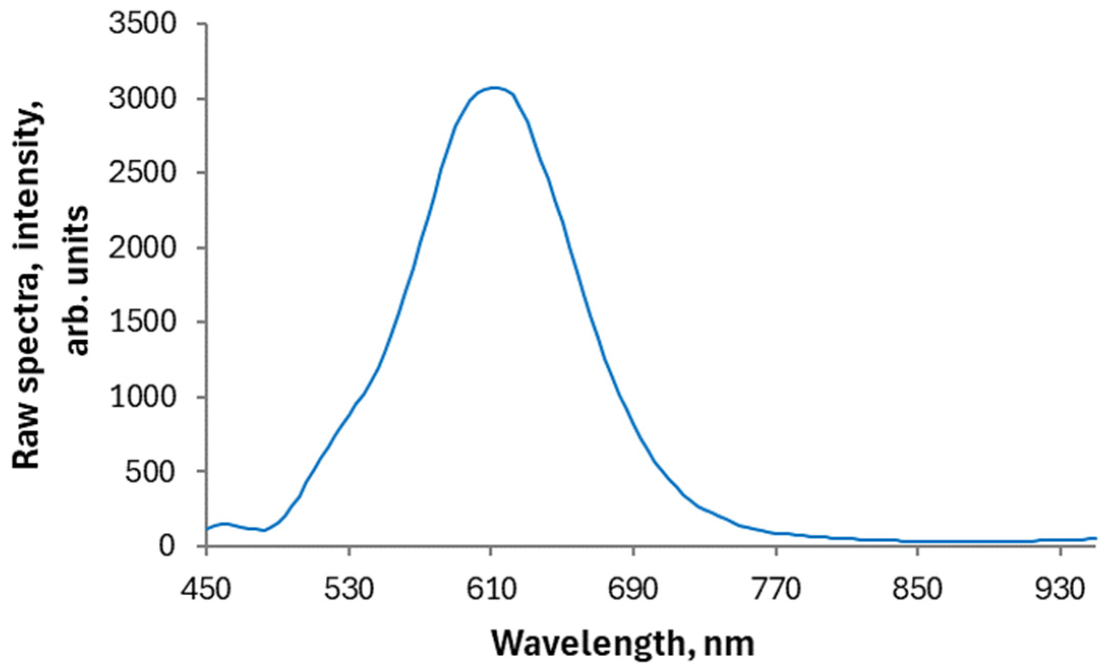
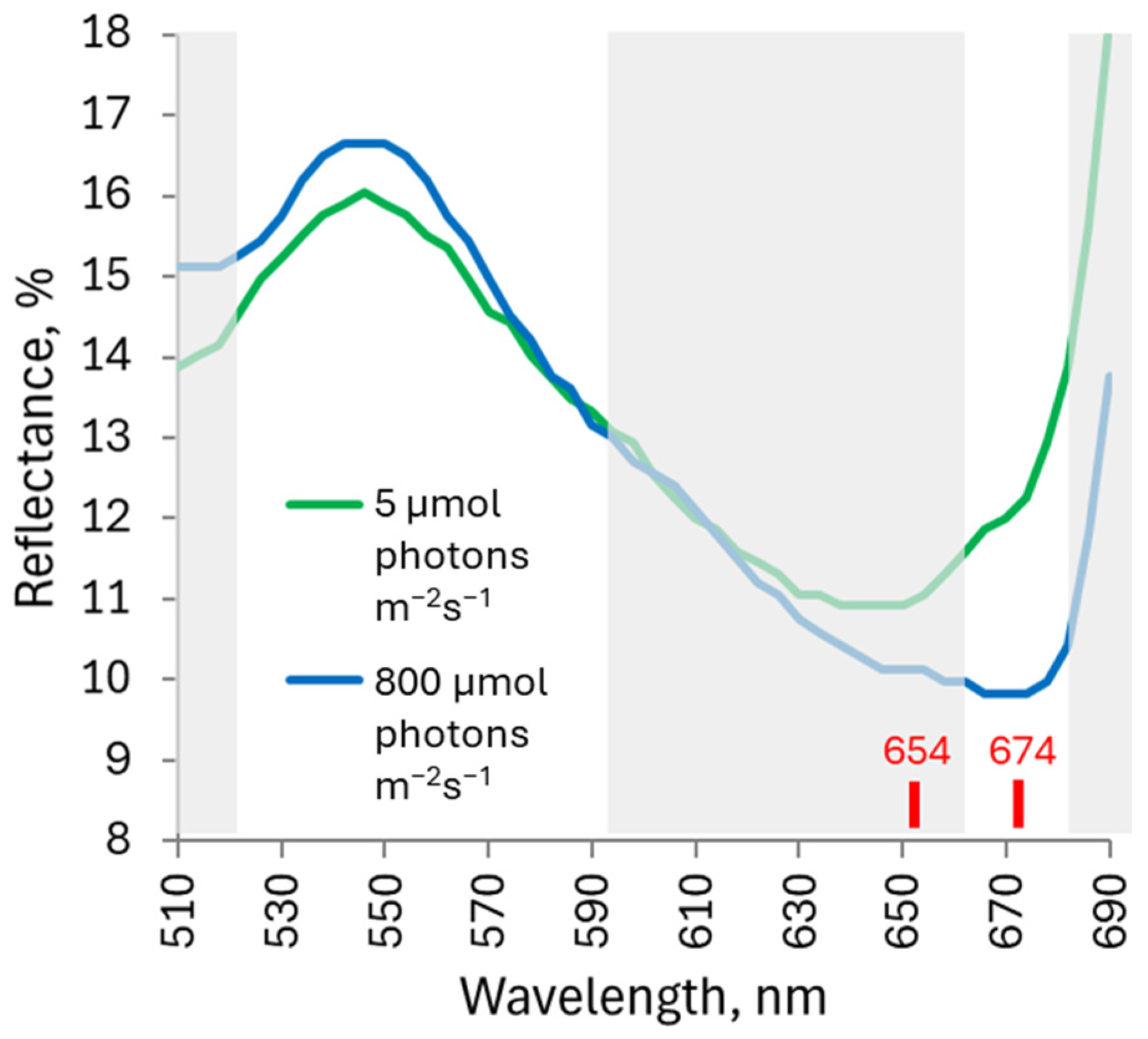
3.1. Character of Changes in the F. elastica Spectral Profiles Induced by the EL Exposure

Figure 2 demonstrates that the EL-induced multidirectional alterations in the spectral profile occurred in the 522–594 and 666–682 nm regions. This finding formed the basis for proposing the LSI vegetation index. Thus, EL led to the noticeable differences in the location of the inflection points of the spectral curve in the red region. For the control plants, the inflection point was detected at 654 nm, whereas it was detected at 674 nm for EL-exposed plants. Based on this, two more vegetation indices were proposed in addition to LSI: LSIRed (R674/R654) and LSINorm ((R674 − R654)/(R674 + R654)).

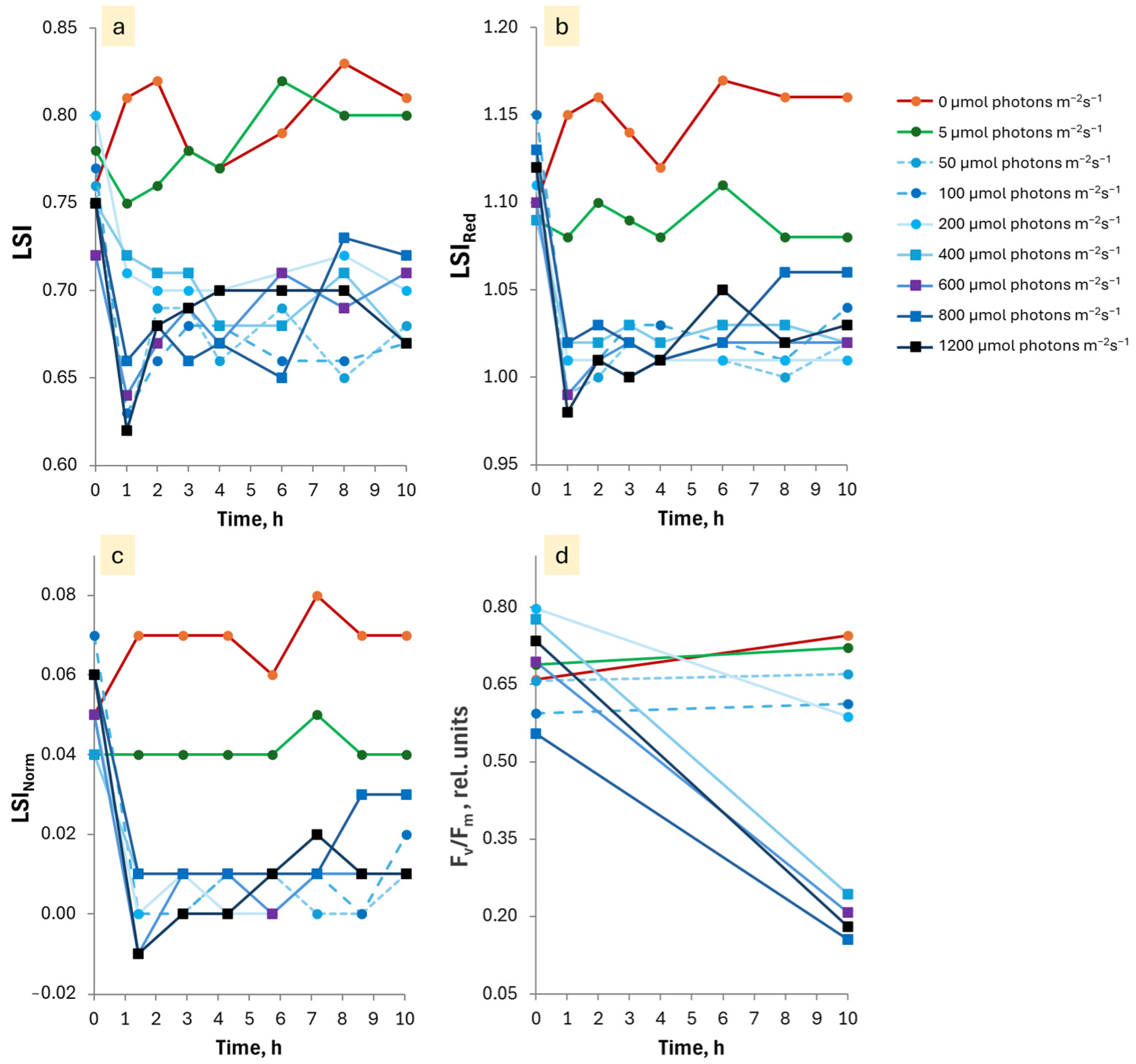
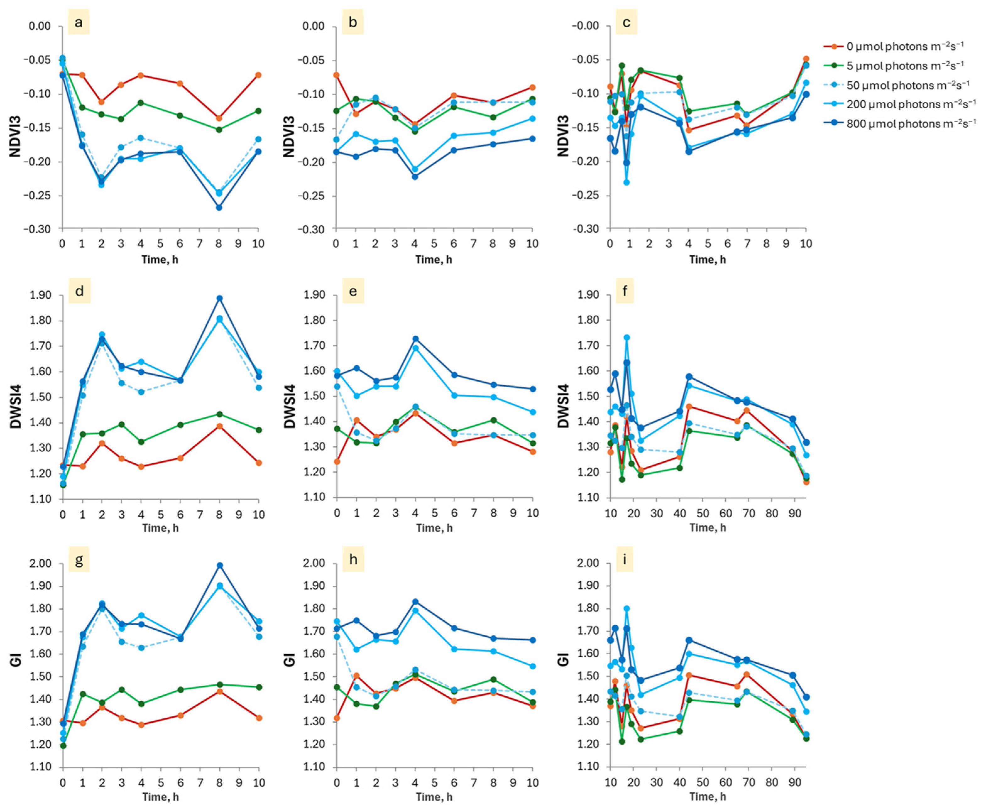
3.2. Dependence of the EL After-Effects on PPFD and Duration of Exposure

The after-effects of EL and LL of different PPFD revealed in F. elastica leaves are shown in Figure 3.
The largest difference in LSI, LSIRed, and LSINorm between the plants exposed to 5 μmol photons m−2s−1 and EL was observed after the first hour of exposure (Figure 3). This difference then became slightly less pronounced. Furthermore, such an EL-after-effect (measured on the basis of LSI, LSIRed, and LSINorm) was independent of PPFD levels in the range from 50 to 1200 μmol photons m−2s−1.
LSI, LSIRed, and LSINorm were found to have different sensitivities to LL exposure. The difference between 5 μmol photons m−2s−1 and LL-exposed plants (0 μmol photons m−2s−1) was small for LSI (Figure 3a), and large for LSIRed and LSINorm (Figure 3b,c). This is the advantage of these two VIs over LSI. The changes in Fv/Fm values (Figure 3d), measured before and after the end of LL and EL exposure, highlights well the PPFD stress range from 400 μmol photons m−2s−1 and above.

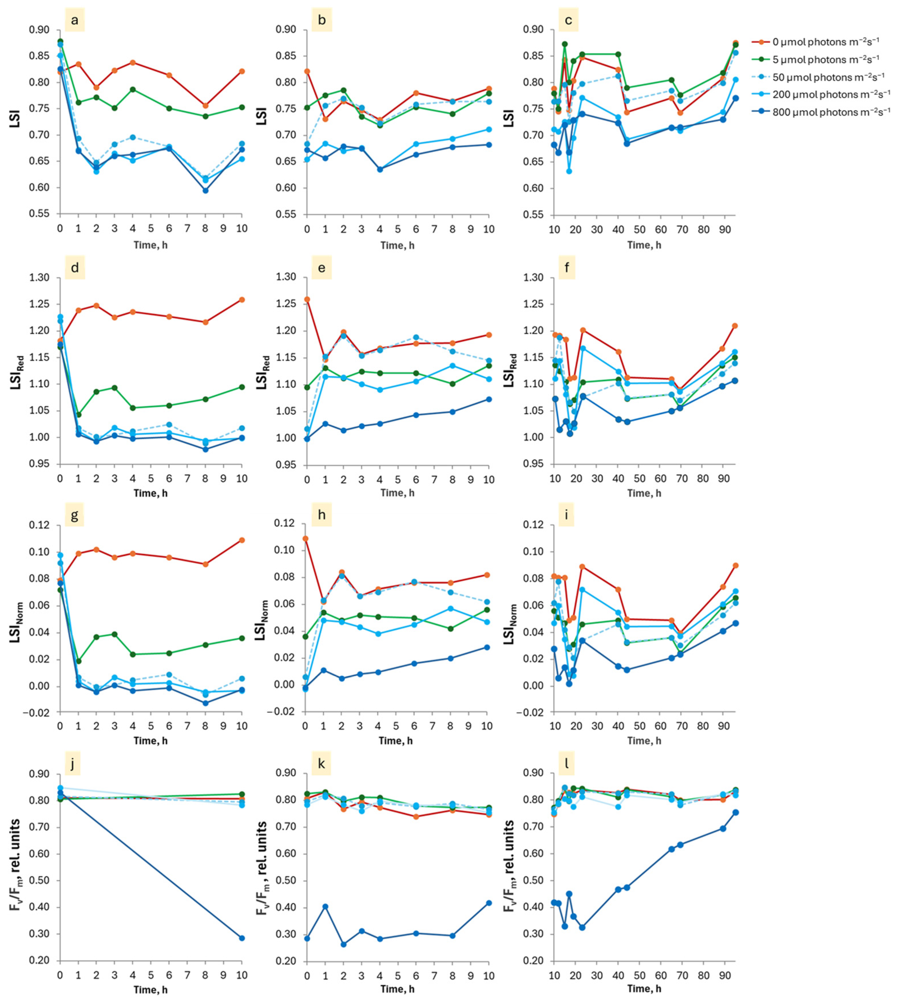
3.3. Duration of the Persistence of the EL and LL After-Effects

The effect of LL exposure was found to have disappeared two hours after cessation of exposure, when LSI, LSIRed, and LSINorm values became equal to those of 5 μmol photons m−2s−1 (Figure 4b,e,h). The persistence of the EL after-effect over time depended on the PPFD level and the VI used. The EL after-effect at the PPFD level of 50 μmol photons m−2s−1 on LSI values disappeared two hours after exposure (Figure 4b). The EL after-effect at PPFD levels of 200 and 800 μmol photons m−2s−1 on LSI values was observed at more than 80 h (Figure 4b,c). The dynamics of the LSIRed and LSINorm values showed prolonged persistence of the EL effect only for PPFD 800 μmol photons m−2s−1 (Figure 4e,f,h,i).
In this regard, the PPFD-dependent Fv/Fm dynamics in F. elastica leaves and its shifts after cessation of exposure are of interest. Only PPFD of 800 μmol photons m2s1 caused significant changes in Fv/Fm values (Figure 4j). This change at the tenth hour of exposure was 0.545 and persisted long after exposure ceased (Figure 4k,l). That is, according to the dynamics of the Fv/Fm value, only this PPFD variant caused stress.

3.4. Comparison of the Response of LSI, LSIRed and LSINorm to Light Stress with Other VIs

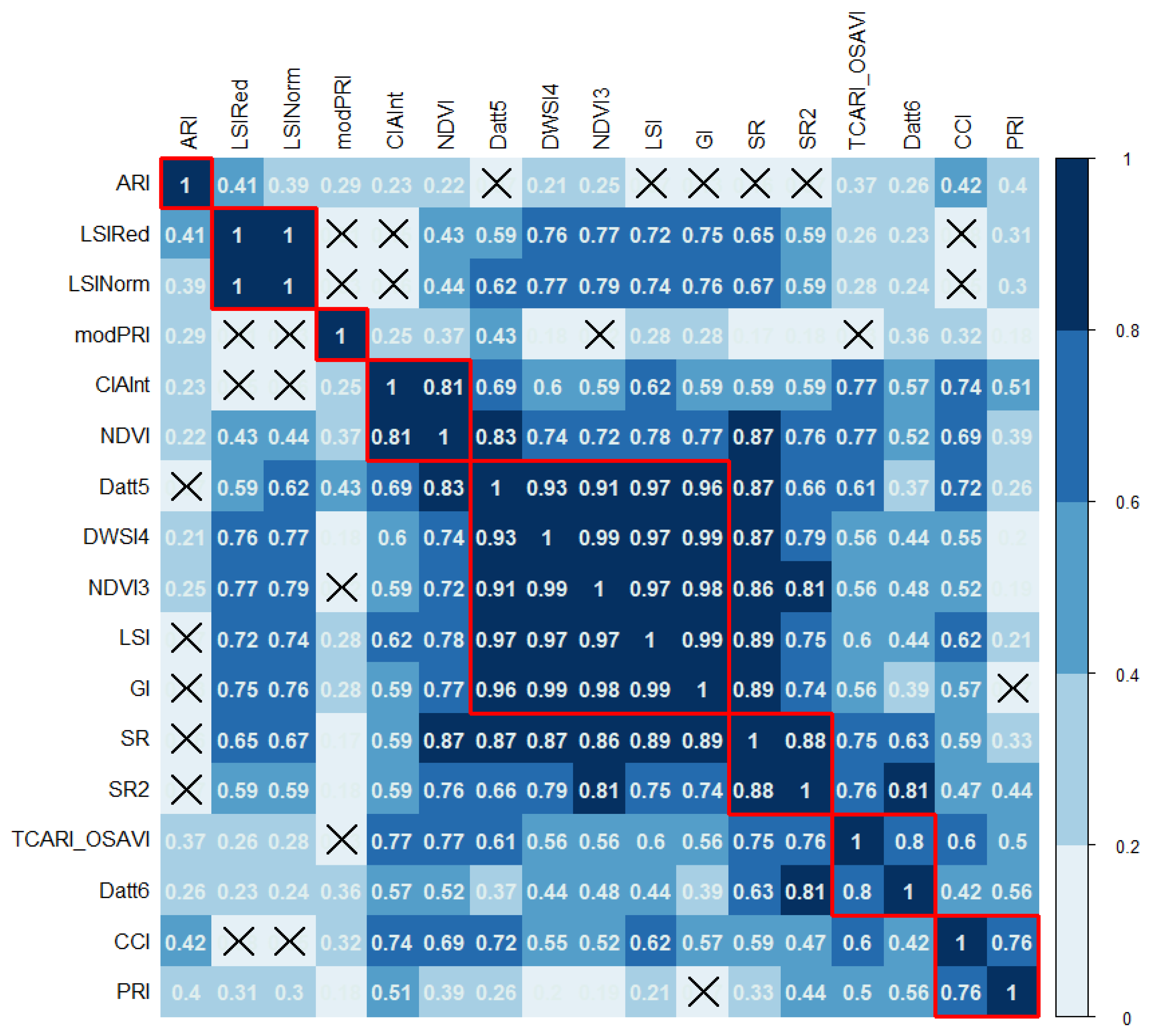
3.4.1. Results of Correlation and Regression Analysis

To evaluate the specific distinguishing features of the proposed VIs, the correlation analysis of the spectral data obtained (see Section 3.3) was performed. Specifically, the aim was to identify the VIs whose response to light stress coincides with that of LSI, LSIRed, and LSINorm. In addition to LSI, LSIRed, and LSINorm, the following VIs were applied as base VIs to construct the correlation matrix: light stress index (modPRI515/550), PRI (used to assess changes in the rapid interconversions of xanthophyll pigments), Anthocyanin Reflectance Index (ARI), CCI, and the most widely used index—Normalized Difference Vegetation Index (NDVI). These VIs were compared with the other 76 VIs presented in Supplementary Table S1. The correlation matrix of vegetation indices is shown in Figure 5. The analysis indicated that LSI had a very high strength of association according to the Cheddock scale (0.90 < r ≤ 0.99) with Datt5, DWSI4, NDVI3, and GI indices. It should be noted that the formulas of these five VIs are similar (Figure 4 and Figure 6, Supplementary Table S1).
The LSIRed and LSINorm VIs also had a high strength of association (0.7 < r ≤ 0.9) with LSI, DWSI4, NDVI3, and GI (Figure 5). The high strength of the relationship between the values of VIs can be explained both by the similarity of their formulas and their common physiological basis—the physiological process occurring in the plant, which is the root cause of changes in the value of a particular VI.
ModPRI, ARI, and PRI, as they had a high strength of association only with CCI, may be considered as unique indices. However, these VIs showed a large scatter of values and no clear patterns across the variants of the experiment. In addition, they correlated poorly with Fv/Fm (Figure 7g–i).

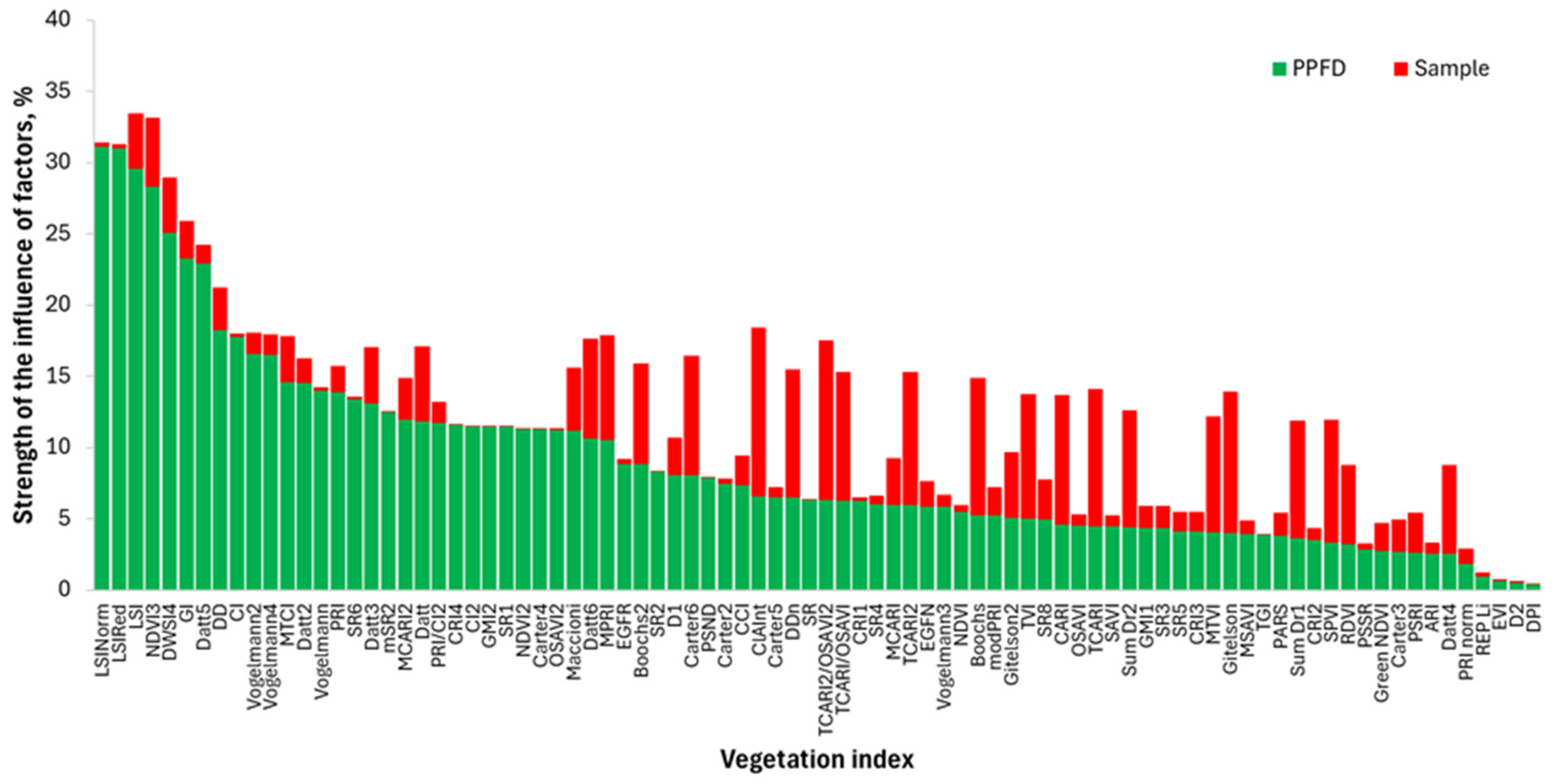
3.4.2. Results of Analysis of Variance

All the VIs discussed in this study were evaluated using two-factor analysis of variance (ANOVA). The first factor was “PPFD” (0 to 1200 μmol photons m−2s−1) and the second factor was “Plant Sample” of F. elastica (three plants were used in each variant). The ANOVA used data after ten of exposure to different levels of PPFD. The results of ANOVA for LSI, LSIRed, and LSINorm are presented in Table 3.
The VIs proposed for the assessment of light stress proved to be very effective for the assessment of light exposure—Sum Sq for the trait “PPFD” was high, and the dependence of the VI value on the PPFD value was highly reliable. This is clearly demonstrated in Figure 8, which shows the strength of the influence of factors (the ratio of the variance of the factor to the total variance, %) LSI, LSIRed, and LSINorm in comparison with other indices.
In addition, the ANOVA results eliminate any doubt regarding the equitability of F. elastica used in the experiment—the influence of variability between individual plant exemplars on the resulting trait, although reliable, is very low in comparison with the influence of PPFD variability.

4. Discussion

Spectral phenotyping of plants is an important approach applied to the biotic and abiotic stress detection currently being used in agriculture. This non-destructive method is based on the registration of electromagnetic radiation reflected by the plant [32].
However, stress detection based on the reflected light spectroscopy of plants has a number of limitations: (1) the high dependence of stress assessment on the species-specific characteristics and environmental conditions [33]; (2) difficulties in distinguishing different types of stress [34]; and (3) difficulties in the stress detection before the visible symptoms appear [35,36].
The results obtained in this study further emphasize the importance of overcoming these challenges in plant stress diagnostics based on the reflected light spectroscopy. The VI formulas employed to assess plant health use wavelengths between 400 and 2500 nm because reflectance in this range is affected by photosynthetic pigments, cell, leaf, canopy structure, and water content [32]. The response of plant pigments (especially chlorophylls, carotenoids, and anthocyanins) to a changing environment is well expressed in the visible region of the reflected electromagnetic spectrum (400–700 nm) [37]. Therefore, plant states (stress, phenological phase, stage of ontogenesis, etc.) are evaluated primarily by VIs through the estimation of photosynthetic pigment content due to the covariance between pigment content and plant state [18]. Thus chlorophyll-sensitive VIs are not specialized in responding to light stress [17].
In the present work, LSI was found to be a good indicator of light stress in Ficus. However, it has been shown to have a very high binding strength to a group of chlorophyll-sensitive VIs (Datt5, DWSI4, NDVI3, and GI) (Figure 5), which calls into question its specificity to light stress.
The Datt5 index has been proposed to estimate the chlorophyll b content of Eucalyptus leaves (while also correlating with chlorophyll a and carotenoids) [38]. The DWSI4 index was proposed to distinguish sugarcane crops severely affected by orange rust disease from those that were not infected [39]. The GI and NDVI3 are structural indices that are sensitive to leaf surface area and leaf chlorophyll content [40]. DWSI4, NDVI3, and GI had relatively high values of R2 with the Fv/Fm value (Figure 7d–f). Despite some differences in the formulas, these VIs appeared to be interchangeable in the presented experiment.
We showed that LSIRed and LSINorm are more specialized to light stress. Although they correlated with NDVI3, DWSI4, GI, and LSI, these indices had a higher dependence on Fv/Fm (Figure 7). LSIRed and LSINorm clearly distinguished between non-stressed (200 μmol photons m−2s−1) and stressed (800 μmol photons m−2s−1) plants (Figure 7e,h). NDVI3, DWSI4, GI, and LSI incorrectly indicated the non-stress exposure of 200 μmol photons m−2s−1 as a stress exposure (Figure 6b,e,h).
A number of other indices are also of great interest for the diagnosis of light stress. In particular, PRI and modPRI515/550 detect rapid interconversions of xanthophyll pigments, thus reflecting one of the mechanisms of plant defense against light stress. Among them also is CCI. It is sensitive to the chlorophyll/carotenoid ratio, which may be changed under prolonged EL exposure [26]. In addition, ARI is an index for estimation of anthocyanin content [41]. However, these indices, working well on other plant species and under other conditions, did not “work” on Ficus under the conditions of our experiment, i.e., they are not universal. It is interesting that modPRI515/550, which was very indicative on maize [26], did not “work” in the case of F. elastica. Together with our data, these facts once again confirm the necessity to develop specific for different types of abiotic stress VIs, which would be universal in relation to plant species.
Thus, the development of VIs capable of assessing certain unique processes of plant defense against light stress is required. This capability would make these VIs unique with respect to the diagnosis of light stress itself. One problem here is that many of the VIs are empirically derived metrics. The LSI, LSIRed, and LSINorm proposed from the study are also empirical. Therefore, the relationship between the values of these VIs and the physiological processes that occur when a plant is exposed to EL requires special studies. The reasons for the observed increase in reflectance in the yellow-green region and decrease in reflectance in the red region with red edge shift under EL action in this study are not clear. Such causes could be changes in pigment concentrations [42] (in particular, xanthoxyl cycle pigments) or light-induced rearrangements of chloroplast localization [8].
In whole, the data obtained showed, that LSI, LSIRed, and LSINorm were the most sensitive to light stress compared to the 81 VIs selected for testing (Supplementary Table S1). At the same time, LSIRed and LSINorm correlated well with the stress indicator Fv/Fm. Therefore, on the one hand, the two new VIs proposed in this study (LSIRed and LSINorm) are more suitable for light stress detection than LSI. On the other hand, LSI, which proved to be more sensitive to EL exposure (LSI is able to detect the after-effect of the non-stressful PPFDs (200 μmol photons m−2s−1)), may be more suitable for the analysis and consideration of the light history of plants. The long-term persistence of the effect of stressed PPFD levels confirms the need to consider the light history of vegetation in its spectral monitoring, as previously pointed out by other authors [43,44].
Limitations and perspectives of the study. The study was performed under the laboratory conditions using proximal hyperspectral imaging at a leaf level. Therefore, it did not address many factors that arise during the remote sensing—spatial resolution, atmospheric characteristics, different levels of canopy PPFD, angle of inclination, etc. The spectral composition of LEDs differs from natural sunlight, which can lead to differences in spectral signatures in artificial and natural light. The study was carried out on a rather highly specialized plant in terms of light conditions—F. elastica. In addition, the formulas of the proposed VIs (LSI, LSIRed, and LSINorm) were derived empirically.
Further research will include (1) testing the proposed VIs on crops and (2) determining the physiological basis of the indices.

5. Conclusions

Exposure of F. elastica leaves to EL results in an increase in reflectance in the yellow-green range and a fall in reflectance in the red range, with a shift of the red edge point towards the longer wavelength.
These changes can be revealed by the proposed VIs: LSI = mean(R666:682)/mean(R522:594), LSIRed = R674/R654 and LSINorm = (R674 − R654)/(R674 + R654). The values of the vegetation indices LSI, LSIRed, and LSINorm are closely correlated with the value of Fv/Fm.
The instantaneous plant response to EL exposure, expressed as VI values, was independent of the PPFD level in the tested range. The effect of EL exposure at the non-stressful PPFD (less than 400 μmol photons m−2s−1) disappeared within one hour after exposure cessation, whereas the effect of stressful PPFD (800 μmol photons m−2s−1) persisted for more than 80 h after exposure cessation.

Supplementary Materials

The following supporting information can be downloaded at: https://www.mdpi.com/article/10.3390/agriengineering6030188/s1, Table S1: Vegetation indices calculated in this study. References [23,26,27,39,40,41,45,46,47,48,49,50,51,52,53,54,55,56,57,58,59,60,61,62,63,64,65,66,67,68,69,70,71,72,73,74,75,76,77,78,79,80,81,82,83,84,85,86,87,88,89] are cited in the supplementary materials.

Author Contributions

Conceptualization, P.A.D., B.L.K. and V.S.L.; Data curation, B.L.K. and A.A.D.; Formal analysis, A.A.D.; Investigation, P.A.D., B.L.K. and A.A.D.; Methodology, P.A.D. and B.L.K.; Project administration, P.A.D.; Resources, V.S.L. and T.V.V.; Software, A.A.D.; Writing—original draft, P.A.D. and B.L.K.; Writing—review and editing, P.A.D., B.L.K. and V.S.L. All authors have read and agreed to the published version of the manuscript.

Funding

The project was supported by the Russian Science Foundation under grant No. 22-14-00338, https://rscf.ru/project/22-14-00338/ (accessed on 7 July 2024), and performed at Southern Federal University (Rostov-on-Don, Russian Federation).

Data Availability Statement

The original contributions presented in the study are included in the article, further inquiries can be directed to the corresponding author.

Conflicts of Interest

The authors declare no conflicts of interest.

References

  1. Zhang, H.; Zhao, Y.; Zhu, J.-K. Thriving under Stress: How Plants Balance Growth and the Stress Response. Dev. Cell 2020, 55, 529–543. [Google Scholar] [CrossRef] [PubMed]
  2. Yadav, S.; Modi, P.; Dave, A.; Vijapura, A.; Patel, D.; Patel, M. Effect of Abiotic Stress on Crops. In Sustainable Crop Production; IntechOpen: London, UK, 2020. [Google Scholar] [CrossRef]
  3. Shi, Y.; Ke, X.; Yang, X.; Liu, Y.; Hou, X. Plants response to light stress. J. Genet. Genom. 2022, 49, 735–747. [Google Scholar] [CrossRef] [PubMed]
  4. Roach, T.; Krieger-Liszkay, A. Regulation of photosynthetic electron transport and photoinhibition. Curr. Protein Pept. Sci. 2014, 15, 351–362. [Google Scholar] [CrossRef] [PubMed]
  5. Takahashi, S.; Badger, M.R. Photoprotection in plants: A new light on photosystem II damage. Trends Plant Sci. 2011, 16, 53–60. [Google Scholar] [CrossRef]
  6. Zhang, M.; Ming, Y.; Wang, H.-B.; Jin, H.-L. Strategies for adaptation to high light in plants. aBIOTECH 2024. [Google Scholar] [CrossRef]
  7. Szymańska, R.; Ślesak, I.; Orzechowska, A.; Kruk, J. Physiological and biochemical responses to high light and temperature stress in plants. Environ. Exp. Bot. 2017, 139, 165–177. [Google Scholar] [CrossRef]
  8. Baránková, B.; Lazár, D.; Nauš, J. Analysis of the effect of chloroplast arrangement on optical properties of green tobacco leaves. Remote Sens. Environ. 2016, 174, 181–196. [Google Scholar] [CrossRef]
  9. Araguirang, G.E.; Richter, A.S. Activation of anthocyanin biosynthesis in high light–what is the initial signal? New Phytol. 2022, 236, 2037–2043. [Google Scholar] [CrossRef]
  10. Nawrocki, W.J.; Tourasse, N.J.; Taly, A.; Rappaport, F.; Wollman, F.-A. The plastid terminal oxidase: Its elusive function points to multiple contributions to plastid physiology. Annu. Rev. Plant Biol. 2015, 66, 49–74. [Google Scholar] [CrossRef]
  11. Curien, G.; Flori, S.; Villanova, V.; Magneschi, L.; Giustini, C.; Forti, G.; Matringe, M.; Petroutsos, D.; Kuntz, M.; Finazzi, G. The water to water cycles in microalgae. Plant Cell Physiol. 2016, 57, 1354–1363. [Google Scholar] [CrossRef]
  12. Rochaix, J.-D. Regulation of photosynthetic electron transport. Biochim. Biophys. Acta 2011, 1807, 375–383. [Google Scholar] [CrossRef] [PubMed]
  13. Lysenko, V.; DRajput, V.; Kumar Singh, R.; Guo, Y.; Kosolapov, A.; Usova, E.; Varduny, T.; Chalenko, E.; Yadronova, O.; Dmitriev, P.; et al. Chlorophyll fluorometry in evaluating photosynthetic performance: Key limitations, possibilities, perspectives and alternatives. Physiol. Mol. Biol. Plants 2022, 28, 2041–2056. [Google Scholar] [CrossRef] [PubMed]
  14. Murata, N.; Nishiyama, Y. ATP is a driving force in the repair of photosystem II during photoinhibition. Plant Cell Environ. 2018, 41, 285–299. [Google Scholar] [CrossRef]
  15. Zeng, Y.; Hao, D.; Huete, A.; Dechant, B.; Berry, J.; Chen, J.M.; Joiner, J.; Frankenberg, C.; Bond-Lamberty, B.; Ryu, Y.; et al. Optical vegetation indices for monitoring terrestrial ecosystems globally. Nat. Rev. Earth Environ. 2022, 3, 477–493. [Google Scholar] [CrossRef]
  16. Xue, J.; Baofeng, S. Significant Remote Sensing Vegetation Indices: A Review of Developments and Applications. J. Sens. 2017, 2017, 1353691. [Google Scholar] [CrossRef]
  17. Ashraf, M.; Harris, P.J.C. Photosynthesis under stressful environments: An overview. Photosynthetica 2013, 51, 163–190. [Google Scholar] [CrossRef]
  18. Wong, C.Y.S. Plant optics: Underlying mechanisms in remotely sensed signals for phenotyping applications. AoB Plants 2023, 15, plad039. [Google Scholar] [CrossRef]
  19. Skendžić, S.; Zovko, M.; Lešić, V.; Pajač Živković, I.; Lemić, D. Detection and Evaluation of Environmental Stress in Winter Wheat Using Remote and Proximal Sensing Methods and Vegetation Indices—A Review. Diversity 2023, 15, 481. [Google Scholar] [CrossRef]
  20. Zhu, K.; Sun, Z.; Zhao, F.; Yang, T.; Tian, Z.; Lai, J.; Zhu, W.; Long, B. Relating Hyperspectral Vegetation Indices with Soil Salinity at Different Depths for the Diagnosis of Winter Wheat Salt Stress. Remote Sens. 2021, 13, 250. [Google Scholar] [CrossRef]
  21. Ihuoma, S.O.; Madramootoo, C.A. Sensitivity of spectral vegetation indices for monitoring water stress in tomato plants. Comput. Electron. Agric. 2019, 163, 104860. [Google Scholar] [CrossRef]
  22. Sanches, I.D.A.; Filho, C.R.S.; Kokaly, R.F. Spectroscopic remote sensing of plant stress at leaf and canopy levels using the chlorophyll 680nm absorption feature with continuum removal. ISPRS J. Photogramm. Remote Sens. 2014, 97, 111–122. [Google Scholar] [CrossRef]
  23. Gamon, J.; Huemmrich, K.; Wong, C.; Ensminger, I.; Garrity, S.; Hollinger, D.; Noormets, A.; Penuelas, J. A remotely sensed pigment index reveals photosynthetic phenology in evergreen conifers. Proc. Natl. Acad. Sci. USA 2016, 113, 201606162. [Google Scholar] [CrossRef]
  24. Gamon, J.; Serrano, L.; Surfus, J. The photochemical reflectance index: An optical indicator of photosynthetic radiation use efficiency across species, functional types, and nutrient levels. Oecologia 1997, 112, 492–501. [Google Scholar] [CrossRef]
  25. Davison, P.; Hunter, C.; Horton, P. Overexpression of β-carotene hydroxylase enhances stress tolerance in Arabidopsis. Nature 2002, 418, 203–206. [Google Scholar] [CrossRef]
  26. Gitelson, A.A.; Zygielbaum, A.I.; Arkebauer, T.J.; Walter-Shea, E.A.; Solovchenko, A. Stress detection in vegetation based on remotely sensed light absorption coefficient. Int. J. Remote Sens. 2024, 45, 259–277. [Google Scholar] [CrossRef]
  27. Dmitriev, P.A.; Kozlovsky, B.L.; Dmitrieva, A.A.; Lysenko, V.S.; Chokheli, V.A.; Varduni, T.V. Indication of Light Stress in Ficus elastica Using Hyperspectral Imaging. AgriEngineering 2023, 5, 2253–2265. [Google Scholar] [CrossRef]
  28. Cun, Z.; Xu, X.Z.; Zhang, J.Y.; Shuang, S.P.; Wu, H.M.; An, T.X.; Chen, J.W. Responses of photosystem to long-term light stress in a typically shade-tolerant species Panax notoginseng. Front. Plant Sci. 2023, 13, 1095726. [Google Scholar] [CrossRef] [PubMed]
  29. Kothari, S.; Montgomery, R.A.; Cavender-Bares, J. Physiological responses to light explain competition and facilitation in a tree diversity experiment. J. Ecol. 2021, 109, 2000–2018. [Google Scholar] [CrossRef]
  30. Poorter, H.; Niinemets, Ü.; Ntagkas, N.; Siebenkäs, A.; Mäenpää, M.; Matsubara, S.; Pons, T. A meta-analysis of plant responses to light intensity for 70 traits ranging from molecules to whole plant performance. New Phytol. 2019, 223, 1073–1105. [Google Scholar] [CrossRef]
  31. Dmitriev, P.A.; Kozlovsky, B.L.; Dmitrieva, A.A.; Varduni, T.V. Classification of invasive tree species based on the seasonal dynamics of the spectral characteristics of their leaves. Earth Sci. Inform. 2023, 16, 3729–3743. [Google Scholar] [CrossRef]
  32. Galieni, A.; D’Ascenzo, N.; Stagnari, F.; Pagnani, G.; Xie, Q.; Pisante, M. Past and Future of Plant Stress Detection: An Overview from Remote Sensing to Positron Emission Tomography. Front. Plant Sci. 2021, 11, 609155. [Google Scholar] [CrossRef] [PubMed]
  33. Zubler, A.V.; Yoon, J.Y. Proximal Methods for Plant Stress Detection Using Optical Sensors and Machine Learning. Biosensors 2020, 10, 193. [Google Scholar] [CrossRef] [PubMed]
  34. Kawamura, K.; Ikeura, H.; Phongchanmaixay, S.; Khanthavong, P. Canopy hyperspectral sensing of paddy fields at the booting stage and PLS regression can assess grain yield. Remote Sens. 2018, 10, 1249. [Google Scholar] [CrossRef]
  35. Reis Pereira, M.; Verrelst, J.; Tosin, R.; Rivera Caicedo, J.P.; Tavares, F.; Neves dos Santos, F.; Cunha, M. Plant Disease Diagnosis Based on Hyperspectral Sensing: Comparative Analysis of Parametric Spectral Vegetation Indices and Nonparametric Gaussian Process Classification Approaches. Agronomy 2024, 14, 493. [Google Scholar] [CrossRef]
  36. Prechsl, U.E.; Mejia-Aguilar, A.; Cullinan, C.B. In vivo spectroscopy and machine learning for the early detection and classification of different stresses in apple trees. Sci. Rep. 2023, 13, 15857. [Google Scholar] [CrossRef] [PubMed]
  37. Blackburn, G.A. Hyperspectral remote sensing of plant pigments. J. Exp. Bot. 2007, 58, 855–867. [Google Scholar] [CrossRef]
  38. Datt, B. Remote Sensing of Chlorophyll a, Chlorophyll b, Chlorophyll a+b, and Total Carotenoid Content in Eucalyptus Leaves. Remote Sens. Environ. 1998, 66, 111–121. [Google Scholar] [CrossRef]
  39. Apan, A.; Held, A.; Phinn, S.; Markley, J. Detecting sugarcane “orange rust” disease using EO-1 Hyperion hyperspectral imagery. Int. J. Remote Sens. 2004, 25, 489–498. [Google Scholar] [CrossRef]
  40. Smith, R.; Adams, J.; Stephens, D.; Hick, P. Forecasting wheat yield in a mediterranean-type environment from the NOAA satellite. Aust. J. Agric. Res. 1995, 46, 113–125. [Google Scholar] [CrossRef]
  41. Gitelson, A.A.; Merzlyak, M.N.; Chivkunova, O.B. Optical properties and nondestructive estimation of anthocyanin content in plant leaves. Photochem. Photobiol. 2001, 74, 38–45. [Google Scholar] [CrossRef]
  42. Laisk, A.; Oja, V.; Eichelmann, H.; Luca Dall’Osto, L. Action spectra of photosystems II and I and quantum yield of photo-synthesis in leaves in State 1. Biochim. Biophys. Acta 2014, 1837, 315–325. [Google Scholar] [CrossRef] [PubMed]
  43. Schmiege, S.C.; Griffin, K.L.; Boelman, N.T.; Vierling, L.A.; Bruner, S.G.; Min, E.; Maguire, A.J.; Jensen, J.; Eitel, J.U.H. Vertical gradients in photosynthetic physiology diverge at the latitudinal range extremes of white spruce. Plant Cell Environ. 2022, 46, 45–63. [Google Scholar] [CrossRef] [PubMed]
  44. Kohzuma, K.; Tamaki, M.; Hikosaka, K. Corrected photochemical reflectance index (PRI) is an effective tool for detecting environmental stresses in agricultural crops under light conditions. J. Plant Res. 2021, 134, 683–694. [Google Scholar] [CrossRef] [PubMed]
  45. Boochs, F.; Kupfer, G.; Dockter, K.; Kuhbauch, W. Shape of the red edge as vitality indicator for plants. Int. J. Remote Sens. 1990, 11, 1741–1753. [Google Scholar] [CrossRef]
  46. Kim, M.; Daughtry, C.; Chappelle, E.; McMurtrey, J.; Walthall, C. The use of high spectral resolution bands for estimating absorbed photosynthetically active radiation (Apar). In Proceedings of the Sixth Symposium on Physical Measurements and Signatures in Remote Sensing, Val d’Isere, France, 17–24 January 1994; Volume 17, pp. 299–306. [Google Scholar]
  47. Carter, G.A. Ratios of leaf reflectances in narrow wavebands as indicators of plant stress. Int. J. Remote Sens. 1994, 15, 697–703. [Google Scholar] [CrossRef]
  48. Zarco-Tejada, P.J.; Pushnik, J.C.; Dobrowski, S.; Ustin, S.L. Steadystate chlorophyll a fluorescence detection from canopy derivative reflectance and double-peak red-edge effects. Remote Sens. Environ. 2003, 84, 283–294. [Google Scholar] [CrossRef]
  49. Gitelson, A.; Gritz, Y.; Merzlyak, M. Relationships between leaf chlorophyll content and spectral reflectance and algorithms for non-destructive chlorophyll assessment in higher plant leaves. J. Plant Physiol. 2003, 160, 271–282. [Google Scholar] [CrossRef]
  50. Oppelt, N.; Mauser, W. Hyperspectral monitoring of physiological parameters of wheat during a vegetation period using AVIS data. Int. J. Remote Sens. 2004, 25, 145–159. [Google Scholar] [CrossRef]
  51. Datt, B. Visible/near infrared reflectance and chlorophyll content in Eucalyptus leaves. Int. J. Remote Sens. 1999, 20, 2741–2759. [Google Scholar] [CrossRef]
  52. Maire, G.; Francois, C.; Dufrene, E. Towards universal broad leaf chlorophyll indices using PROSPECT simulated database and hyperspectral reflectance measurements. Remote Sens. Environ. 2004, 89, 1–28. [Google Scholar] [CrossRef]
  53. Penuelas, J.; Gamon, J.A.; Fredeen, A.L.; Merino, J.; Field, C.B. Reflectance indices associated with physiological-changes in nitrogen-limited and water-limited sun ower leaves. Remote Sens. Environ. 1994, 48, 135–146. [Google Scholar] [CrossRef]
  54. Huete, A.; Liu, H.Q.; Batchily, K.; van Leeuwen, W. A comparison of vegetation indices over a global set of TM images for EOS–MODIS. Remote Sens. Environ. 1997, 59, 440–451. [Google Scholar] [CrossRef]
  55. Gitelson, A.; Buschmann, C.; Lichtenthaler, H. The chlorophyll fluorescence ratio F735/F700 as an accurate measure of the chlorophyll content in plants—Experiments with autumn chestnut and maple leaves. Remote Sens. Environ. 1999, 69, 296–302. [Google Scholar] [CrossRef]
  56. Gitelson, A.A.; Kaufman, Y.J.; Merzlyak, M.N. Use of a green channel in remote sensing of global vegetation from EOS-MODIS. Remote Sens. Environ. 1996, 58, 289–298. [Google Scholar] [CrossRef]
  57. Maccioni, A.; Agati, G.; Mazzinghi, P. New vegetation indices for remote measurement of chlorophylls based on leaf directional reflectance spectra. J. Photochem. Photobiol. B Biol. 2001, 61, 52–61. [Google Scholar] [CrossRef] [PubMed]
  58. Daughtry, C.; Walthall, C.; Kim, M.; Brown de Colstoun, E.; McMurtrey, J.E., III. Estimating corn leaf chlorophyll concentration from leaf and canopy reflectance. Remote Sens. Environ. 2000, 74, 229–239. [Google Scholar] [CrossRef]
  59. Hernandez-Clemente, R.; Navarro-Cerrillo, R.M.; Suarez, L.; Morales, F.; Zarco-Tejada, P.J. Assessing structural effects on PRI for stress detection in conifer forests. Remote Sens. Environ. 2011, 115, 2360–2375. [Google Scholar] [CrossRef]
  60. Qi, J.; Chehbouni, A.; Huete, A.; Kerr, Y.; Sorooshian, S. A modified soil adjusted vegetation index. Remote Sens. Environ. 1994, 48, 119–126. [Google Scholar] [CrossRef]
  61. Chen, J.M. Evaluation of vegetation indices and a modified simple ratio for boreal applications. Can. J. Remote Sens. 1996, 22, 229–242. [Google Scholar] [CrossRef]
  62. Dash, J.P.; Curran, P.J. The MERIS terrestrial chlorophyll index. Int. J. Remote Sens. 2004, 25, 5403–5413. [Google Scholar] [CrossRef]
  63. Haboudane, D.; Miller, J.R.; Pattey, E.; Zarco-Tejada, P.J.; Strachan, I.B. Hyperspectral vegetation indices and novel algorithms for predicting green LAI of crop canopies: Modeling and validation in the context of precision agriculture. Remote Sens. Environ. 2004, 90, 337–352. [Google Scholar] [CrossRef]
  64. Tucker, C.J. Red and photographic infrared linear combinations for monitoring vegetation. Remote Sens. Environ. 1979, 8, 127–150. [Google Scholar] [CrossRef]
  65. Gitelson, A.; Merzlyak, M.N. Quantitative estimation of chlorophyll-a using reflectance spectra: Experiments with autumn chestnut and maple leaves. J. Photochem. Photobiol. B Biol. 1994, 22, 247–252. [Google Scholar] [CrossRef]
  66. Gandia, S.; Fernandez, G.; Garcia, J.; Moreno, J. Retrieval of vegetation biophysical variables from CHRIS/PROBA data in the SPARC campaign. In Proceedings of the ESA SP-578, 2nd CHRIS/Proba Workshop, ESA/ESRIN, Frascati, Italy, 28–30 April 2004; pp. 40–48. [Google Scholar]
  67. Rondeaux, G.; Steven, M.; Baret, F. Optimization of soil-adjusted vegetation indices. Remote Sens. Environ. 1996, 55, 95–107. [Google Scholar] [CrossRef]
  68. Wu, C.; Niu, Z.; Tang, Q.; Huang, W. Estimating chlorophyll content from hyperspectral vegetation indices: Modeling and validation. Agric. For. Meteorol. 2008, 148, 1230–1241. [Google Scholar] [CrossRef]
  69. Chappelle, E.W.; Kim, M.S.; McMurtrey, J.E. Ratio analysis of reflectance spectra (rars)—An algorithm for the remote estimation of the concentrations of chlorophyll-a, chlorophyll-b, and carotenoids in soybean leaves. Remote Sens. Environ. 1992, 39, 239–247. [Google Scholar] [CrossRef]
  70. Gamon, J.; Penuelas, J.P.; Field, C. A narrow-waveband spectral index that tracks diurnal changes in photosynthetic efficiency. Remote Sens. Environ. 1992, 41, 35–44. [Google Scholar] [CrossRef]
  71. Zarco-Tejada, P.J.; Gonzalez-Dugo, V.; Williams, L.E.; Suarez, L.; Berni, J.A.J.; Goldhamer, D.; Fereres, E. A PRI-based water stress index combining structural and chlorophyll effects: Assessment using diurnal narrow-band airborne imagery and the CWSI thermal index. Remote Sens. Environ. 2013, 138, 38–50. [Google Scholar] [CrossRef]
  72. Garrity, S.R.; Eitel, J.U.; Vierling, L.A. Disentangling the relationships between plant pigments and the photochemical reflectance index reveals a new approach for remote estimation of carotenoid content. Remote Sens. Environ. 2011, 115, 628–635. [Google Scholar] [CrossRef]
  73. Merzlyak, M.N.; Gitelson, A.A.; Chivkunova, O.B.; Rakitin, V.Y. Non-destructive optical detection of pigment changes during leaf senescence and fruit ripening. Physiol. Plant. 1999, 106, 135–141. [Google Scholar] [CrossRef]
  74. Blackburn, G.A. Quantifying chlorophylls and caroteniods at leaf and canopy scales: An evaluation of some hyperspectral approaches. Remote Sens. Environ. 1998, 66, 273–285. [Google Scholar] [CrossRef]
  75. Roujean, J.L.; Breon, F.M. Estimating par absorbed by vegetation from bidirectional reflectance measurements. Remote Sens. Environ. 1995, 51, 375–384. [Google Scholar] [CrossRef]
  76. Guyot, G.; Baret, F. Utilisation de la haute resolution spectrale pour suivre l’etat des couverts vegetaux. Spectr. Signat. Objects Remote Sens. 1988, 287, 279–286. [Google Scholar]
  77. Huete, A. A soil-adjusted vegetation index (SAVI). Remote Sens. Environ. 1988, 25, 295–309. [Google Scholar] [CrossRef]
  78. Vincini, M.; Frazzi, E.; D’Alessio, P. Angular dependence of maize and sugar beet VIs from directional CHRIS/PROBA data. In Proceedings of the 4th ESA CHRIS PROBA Workshop, Frascati, Italy, 19–21 September 2006; Volume 1, pp. 19–21. [Google Scholar]
  79. Jordan, C.F. Derivation of leaf-area index from quality of light on forest floor. Ecology 1969, 50, 663–678. [Google Scholar] [CrossRef]
  80. Gitelson, A.A.; Merzlyak, M.N. Remote estimation of chlorophyll content in higher plant leaves. Int. J. Remote Sens. 1997, 18, 2691–2697. [Google Scholar] [CrossRef]
  81. McMurtrey, J.E.; Chappelle, E.W.; Kim, M.S.; Meisinger, J.J.; Corp, L.A. Distinguishing nitrogen-fertilization levels in-field corn (Zea mays L) with actively induced fluorescence and passive reflectance measurements. Remote Sens. Environ. 1994, 47, 36–44. [Google Scholar] [CrossRef]
  82. Zarco-Tejada, P.J.; Miller, J.R. Land cover mapping at BOREAS using red edge spectral parameters from CASI imagery. J. Geophys. Res.-Atmos. 1999, 104, 27921–27933. [Google Scholar]
  83. Hernandez-Clemente, R.; Navarro-Cerrillo, R.M.; Zarco-Tejada, P.J. Carotenoid content estimation in a heterogeneous conifer forest using narrowband indices and PROSPECT + DART simulations. Remote Sens. Environ. 2012, 127, 298–315. [Google Scholar] [CrossRef]
  84. Elvidge, C.D.; Chen, Z.K. Comparison of broad-band and narrow-band red and near-infrared vegetation indices. Remote Sens. Environ. 1995, 54, 38–48. [Google Scholar] [CrossRef]
  85. Filella, I.; Penuelas, J. The red edge position and shape as indicators of plant chlorophyll content, biomass, and hydric status. Int. J. Remote Sens. 1994, 15, 1459–1470. [Google Scholar] [CrossRef]
  86. Haboudane, D.; Miller, J.R.; Tremblay, N.; Zarco-Tejada, P.J.; Dextraze, L. Integrated narrow-band vegetation indices for prediction of crop chlorophyll content for application to precision agriculture. Remote Sens. Environ. 2002, 81, 416–426. [Google Scholar] [CrossRef]
  87. Hunt, E.R.; Doraiswamy, P.C.; McMurtrey, J.E.; Daughtry, C.S.; Perry, E.M.; Akhmedov, B. A visible band index for remote sensing leaf chlorophyll content at the canopy scale. Int. J. Appl. Earth Obs. Geoinf. 2013, 21, 103–112. [Google Scholar] [CrossRef]
  88. Broge, N.; Leblanc, E. Comparing prediction power and stability of broadband and hyperspectral vegetation indices for estimation of green leaf area index and canopy chlorophyll density. Remote Sens. Environ. 2000, 76, 156–172. [Google Scholar] [CrossRef]
  89. Vogelmann, J.E.; Rock, B.N.; Moss, D.M. Red edge spectral measurements from sugar maple leaves. Int. J. Remote Sens. 1993, 14, 1563–1575. [Google Scholar] [CrossRef]
Figure 1. Spectrum of white LEDs in the range from 450 to 950 nm.
Agriengineering 06 00188 g001
Figure 2. Spectral profiles of F. elastica leaves exposed to 5 μmol photons m−2s−1 and EL (800 μmol photons m−2s−1) for 10 h. Vertical white stripes indicate the ranges used for LSI calculation and red bars indicate inflection points (nm).
Agriengineering 06 00188 g002
Figure 3. Values of vegetation indices LSI (a); LSIRed (b); LSINorm (c) and Fv/Fm (d) of F. elastica leaves exposed to different PPFD during 10 h.
Agriengineering 06 00188 g003
Figure 4. LSI, LSIRed, LSINorm, and Fv/Fm dynamics measured in F. elastica leaves after exposure at different PPFD levels. During exposure to PPFD (a,d,g,j); first 10 h after cessation of PPFD exposure (b,e,h,k), period 10 to 90 h after cessation of PPFD exposure (c,f,i,l).
Agriengineering 06 00188 g004
Figure 5. Correlation matrix of LSI, LSIRed, LSINorm, and commonly applied VIs (in absolute values) measured in F. elastica leaves after ten hours of exposure at different PPFD levels and after the cessation of exposure (see Section 3.3). Crosses indicate non-significant (p ≥ 0.01) correlation. The red frame indicates groups of VIs obtained as a result of hierarchical clustering.
Agriengineering 06 00188 g005
Figure 6. NDVI3, DWSI4, and GI dynamics measured in F. elastica leaves after exposure at different PPFD levels. During exposure to PPFD (a,d,g); first 10 h after cessation of PPFD exposure (b,e,h), period 10 to 90 h after cessation of PPFD exposure (c,f,i).
Agriengineering 06 00188 g006
Figure 7. Regression plots between Fv/Fm and LSI (a), LSIRed (b), LSINorm (c), DWSI4 (d), GI (e), NDVI3 (f), ARI (g), CCI (h), and modPRI (i). Measurements were performed in F. elastica leaves after ten hours of exposure to EL (800 μmol photons m−2s−1) and after cessation of exposure (see Section 3.3).
Agriengineering 06 00188 g007
Figure 8. The strength of influence of “PPFD” and “Sample” factors on VI values.
Agriengineering 06 00188 g008
Table 1. Dependence of F. elastica leaf temperature depending on PPFD value and air ventilation, °C.
Measurement VariantPPFD, μmol Photons m−2s−1
05501002004006008001200
No ventilation25.025.026.927.328.028.829.229.931.7
VentilatedNANA25.025.527.027.227.327.527.8
Table 2. The schedule of the experiments and timeline application of different PPFD levels.
Date of ExperimentPPFD, μmol Photons m−2s−1
05501002004006008001200
26 January 2024XX XX
2 February 2024 X X XX
8 February 2024 XXXX
9 February 2024XX XX
16 February 2024 XX X X
Table 3. Results of two-factor ANOVA for LSI, LSIRed, and LSINorm (significant at the p ≤ 0.001 level).
LSI
FactorDfSum SqMean SqF value
PPFD86.2170.777135.500
Sample20.8180.40971.300
PPFD & Sample161.1650.07312.700
Residuals223612.8200.006
LSINorm
FactorDfSum SqMean SqF value
PPFD81.0880.136133.651
Sample20.0110.0065.595
PPFD & Sample160.1210.0087.444
Residuals22362.2750.001
LSIRed
FactorDfSum SqMean SqF value
PPFD85.2260.653132.893
Sample20.0490.0244.951
PPFD & Sample160.5840.0377.426
Residuals223610.9910.005
Disclaimer/Publisher’s Note: The statements, opinions and data contained in all publications are solely those of the individual author(s) and contributor(s) and not of MDPI and/or the editor(s). MDPI and/or the editor(s) disclaim responsibility for any injury to people or property resulting from any ideas, methods, instructions or products referred to in the content.

