Automated Windrow Profiling System in Mechanized Peanut Harvesting

Abstract

In peanut cultivation, the fact that the fruits develop underground presents significant challenges for mechanized harvesting, leading to high loss rates, with values that can exceed 30% of the total production. Since the harvest is conducted indirectly in two stages, losses are higher during the digging/inverter stage than the collection stage. During the digging process, losses account for about 60% to 70% of total losses, and this operation directly influences the losses during the collection stage. Experimental studies in production fields indicate a strong correlation between losses and the height of the windrow formed after the digging/inversion process, with a positive correlation coefficient of 98.4%. In response to this high correlation, this article presents a system for estimating the windrow profile during mechanized peanut harvesting, allowing for the measurement of crucial characteristics such as the height, width and shape of the windrow, among others. The device uses an infrared laser beam projected onto the ground. The laser projection is captured by a camera strategically positioned above the analyzed area, and through advanced image processing techniques using triangulation, it is possible to measure the windrow profile at sampled points during a real experiment under direct sunlight. The technical literature does not mention any system with these specific characteristics utilizing the techniques described in this article. A comparison between the results obtained with the proposed system and those obtained with a manual profilometer showed a root mean square error of only 28 mm. The proposed system demonstrates significantly greater precision and operates without direct contact with the soil, making it suitable for dynamic implementation in a control mesh for a digging/inversion device in mechanized peanut harvesting and, with minimal adaptations, in other crops, such as beans and potatoes.

1. Introduction

Climate change, natural disasters and desertification have made agricultural production increasingly challenging. In addition, the increase in the world’s population has increased the demand for food to an unprecedented extent. New strategies and technologies strongly based on agricultural automation are needed, seeking to optimize production and minimize losses in a context of sustainability. Precision agriculture is a viable means of achieving these goals. In this context, the acquisition of data for sensing in agricultural areas has traditionally been performed using satellite images and unmanned aerial vehicles. These images provide a view of the upper part of the crop.

In more recent applications, mobile land robots have also been used in monitoring and mapping tasks, as they have abilities to acquire data from plants and crops at different observation points, combined with a large payload capacity. They are also more robust to weather conditions and are not subject to specific laws and regulations, in contrast to unmanned aerial vehicles.

According to Fasiolo et al. [1], various robotic platforms have been developed by the academic community and agricultural companies. They can basically be grouped into custom mobile robots [2,3,4,5,6,7,8,9], sensorized agricultural machines [10,11] and commercial solutions [12,13,14]. The use of these platforms in precision agriculture involves analyzing data to make cultivation more efficient, with fewer harvest losses and, consequently, better use of natural resources.

Among agricultural mechanized systems, harvesting is considered one of the most relevant and crucial stages, as it ensures the return on investment made in all stages of production. As the penultimate mechanized operation in the peanut production system, digging is challenging due to the interaction between various factors related to cultivation, such as soil conditions, harvest time, climate, crop health, and maturation, as well as those related to machinery, like travel speed and adjustments, which affect the quality of this operation. In Brazil, losses found at this stage are very high, ranging from 3.1 to 47.1% of productivity [15,16,17,18,19], with the digging stage being responsible for most of the total loss.

Therefore, it is necessary to establish adequate working conditions to minimize these losses and ensure the economic viability of the crop. In this regard, diggers/inverters must be well-adjusted so that the windrows are well-aligned and of adequate dimensions to reduce losses.

The peanut (Arachis hypogaea L.) is of great importance on the global agricultural scene. The largest peanut producers are China and the United States. Approximately 55 million tons are produced annually in the world in a planted area of around 32 million hectares [20].

Brazil and Argentina are the largest peanut producers in South America. In Brazil alone, about 730.000 tons were produced in 2023. This volume is mainly the product of an increase in mechanization of the steps in harvesting. This reduces losses during the global process.

Due to the fact that pods are formed below the soil surface, peanut harvesting is carried out indirectly, i.e., it requires the use of more than one machine to carry out the different stages of the process. Harvesting is carried out in two distinct phases, called digging and collection. The digging stage is carried out by a machine called a digger–inverter. This machine has two blades that cut the root of the peanut plants. The cut plants are placed on a vibrating belt driven by a shaft derived from the tractor engine that drives the mechanism. Plants are then inverted and deposited in the soil, forming a windrow. Figure 1 details the digger–inverter mechanism. Losses occur in this process. Invisible Losses are related to the pods that remain below the soil during the digging process, and visible losses are related to the pods that are deposited on the soil during the inversion process (some peanuts fall when passing through the conveyor belt). These losses represent between 30% and 47% of production, and minimizing them could result in a significant increase in the producer’s productivity and earnings [21].

There are several works related to techniques for minimizing losses in the peanut digging process. Ortiz [22] studied the effect of digging machine deviations around the midline of the windrow on peanut productivity and quality. He also determined the economic impact of using tractors with automatic guidance systems in harvesting operations. The authors experimentally proved that the use of these systems results in higher yield rates, as their data showed that for each row deviation of 20 mm, an average loss of 186 kg/ha is expected.

Santos [21] studied the impact of digger-blade wear on the peanut digging process. A possible correlation between the blades of the digging mechanism (the wear of these blades) and the losses that occur during the harvesting process (digging) was studied, considering different harvesting periods (morning, afternoon and night). This study showed that there was no correlation between working periods and losses in the peanut harvest. However, they showed that wear on the blades of the digging equipment results in a major increase in losses. As a result of the experiment, the authors concluded that there could be an increase of up to 22% in profitability due to the reduction in excavation losses, just by conveniently changing the blades during the excavation process.

Yang [23] studied the problem of high loss rates in the peanut harvest in China. He focused on studying the flow selection device of the harvesting machine. Project parameters were defined for the components of the harvesting machine, involving aspects related to the quantity of plants fed onto the belt and the speed of the tangential and axial cylinders, seeking to reduce losses in the peanut digging process.

Shi [24] studied the correlation between the peanut harvesting process and the mechanical properties of peanuts. Tests were carried out on a mechanized harvesting device to evaluate various parameters, such the speed of the harvesting cylinder, the plant-feeding volume, etc. Through field tests, the parameters for maximum performance were obtained. The authors proposed a comprehensive scheme for reducing losses and optimizing the harvesting process based on the obtained results.

Azmoodeh-Mishamandani et al. [25] studied the correlation between pod losses in peanut harvesting and soil moisture content, as well as between the forward speed and conveyor belt inclination in a digger machine. Results showed a significant correlation between different pod losses and soil moisture content and forward speed, while the effect of conveyor inclination was not significant. The authors concluded that it is possible to reduce total loss rates by reducing the loss of unexposed pods by controlling soil moisture content at harvest. The results also revealed that the loss of exposed fruit can be minimized by using the minimum conveyor inclination at the minimum forward speed and vice-versa.

Shen et al. [20] analyzed the correlation between harvesting methods and peanut digging and inversion techniques in China and other countries. They carried out an experiment using digger–inverter to evaluate the inversion rate, buried pod rate and fallen pod rate as a function of tractor travel speed, conveyor chain speed and inverter roller line speed. According to the authors, the obtained experimental results can be used to optimize digger–inverter equipment through the implementation of data collection relating to the process.

Ferezin [26] evaluated visible, invisible and total losses and operational performance in mechanized peanut harvesting related to different PTO (tractor power take-off) speeds. The authors concluded that there was no influence of PTO speed on the average visible, invisible and total losses during digging.

Bunhola [27] evaluated the relationship between windrow height and visible losses in the mechanized harvesting of peanuts and found that these two parameters showed a positive correlation. The authors concluded that the higher the windrow height, the higher the visible losses in the harvesting process.

Based on the results obtained in [27], the need for a system capable of estimating the height of the windrow formed during the peanut harvesting process was identified in order to provide the excavator operator with information for dynamic process adjustments. This information can enable the operator to make the necessary in-field adjustments, and since mechanized harvesting involves high variability in the factors that affect the process and, consequently, the harvest losses, dynamic adjustment of the settings becomes essential to minimize losses and, consequently, increase the efficiency of the operation.

In order to estimate windrow height in an automated way, it is necessary to carry out three-dimensional reconstruction. Three-dimensional reconstruction methods are an important field in engineering and can be grouped into the following two distinct groups: methods used in computer-aided design/computer-aided engineering integration environments (CAD/CAM), 3D printing, virtual reality and augmented reality [28] and methods used to analyze physical 3D profiles. The latter can be divided into three categories [29,30,31,32] according to the way in which the data are acquired. The first category includes algorithms based on stereoscopic vision that observe the scene through two or more simultaneous views. Depth information is obtained by estimating the distance of the same point in the two images. However, depending on the complexity of the scene, finding corresponding points can be a challenging task. The second category includes methods based on the propagation time of a wave pulse (Time of Flight or ToF), usually in the form of light. The distance is calculated from the time measured between the emission of the pulse and its return after reflecting off a point of interest. Reconstruction applications using this method typically use LiDAR (Light Detection and Ranging) sensors. The last category comprises methods based on structured light, in which the projection of a light pattern onto the scene is used to estimate the depth from the distortions of the light pattern in the image. This last method, based on structured light projection, is very suitable for agricultural areas and their peculiarities. There is no mention in the literature of a three-dimensional reconstruction system based on a laser beam for use in analyzing the windrow profile resulting from the peanut digging process.

The combination of the monitoring and mapping potential of mobile agricultural robots with the possibility of working on the ground to improve harvests is the focus of this article, as it provides a solution for dynamically monitoring the height of the windrow resulting from the digging process, consequently providing real-time information to the driver of the digger–inverter mechanism, allowing losses in the peanut harvest to be minimized. The use of automated mapping of the windrow profile to dynamically adjust the grubbing equipment and, consequently, reduce losses has not been mentioned in the specialized literature in the area and is, therefore, a new application for the involved computational process, as well as for the utilized engineering solution.

In this context, this work describes the use of a sensor based on the triangulation of the projection, in image, of a beam produced from an infrared laser, allowing the profile of the windrow to be determined using a scanning strategy by means of the displacement of a robot, or coupled with the digger–inverter equipment. This strategy allows the profile of the windrow to be analyzed during the digging operation. Detailing the dimensions of the windrow can help to estimate productivity and losses. In addition, the correlation between the dimensions of the windrow and the losses obtained in the peanut production process can provide performance parameters, allowing operations to be improved. The proposed system, when used in a georeferenced way, makes it possible to carry out a sectorized productivity study within the guidelines of precision agriculture. The use of the proposed system can be extended to different crops with similar characteristics to help in tasks such as crop analysis, production estimation and pest control.

The proposed system was tested in a real experiment, and the obtained data were compared with those obtained using a manual profilometer (a device traditionally used for this purpose). The obtained results demonstrate its viability.

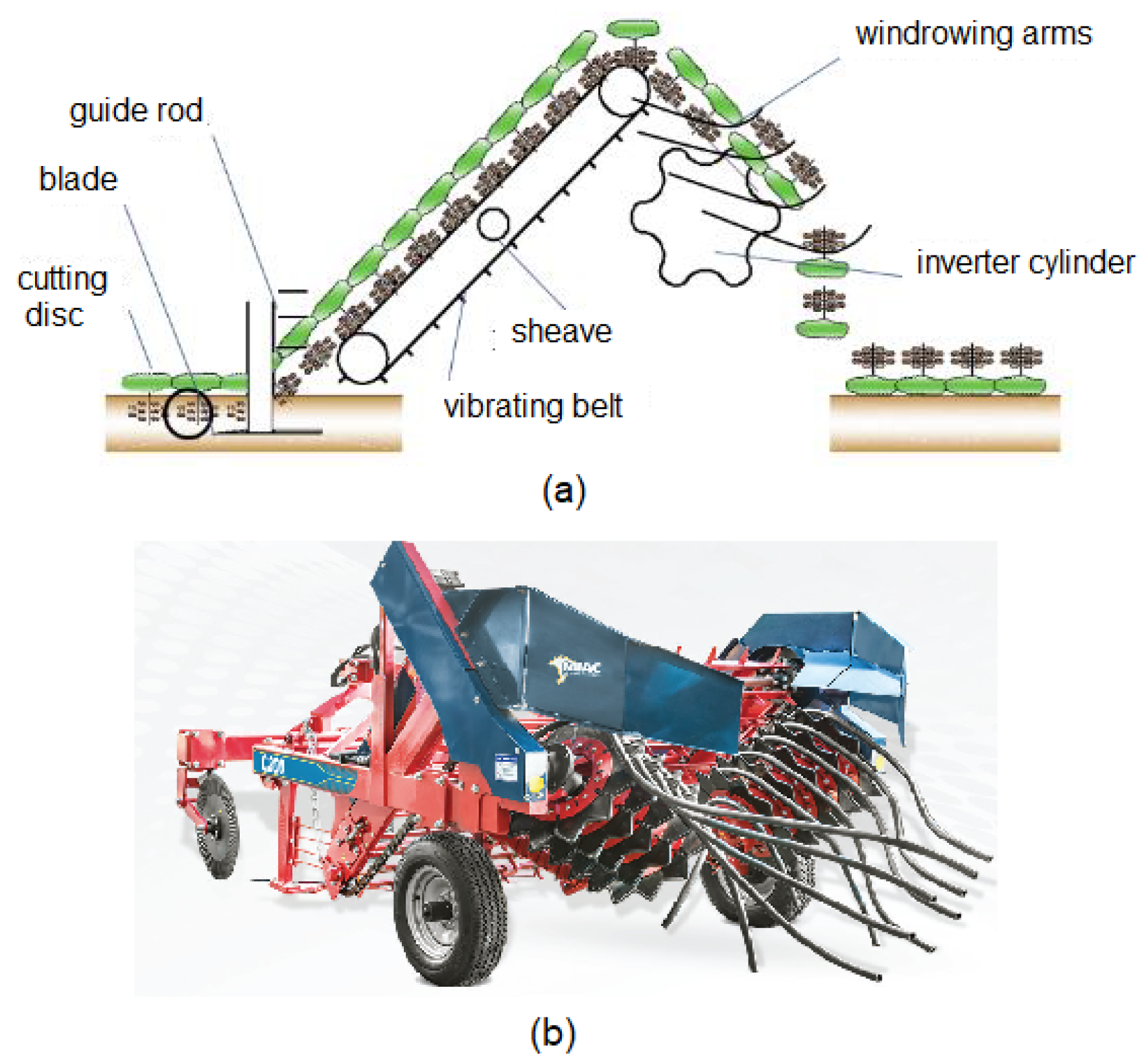
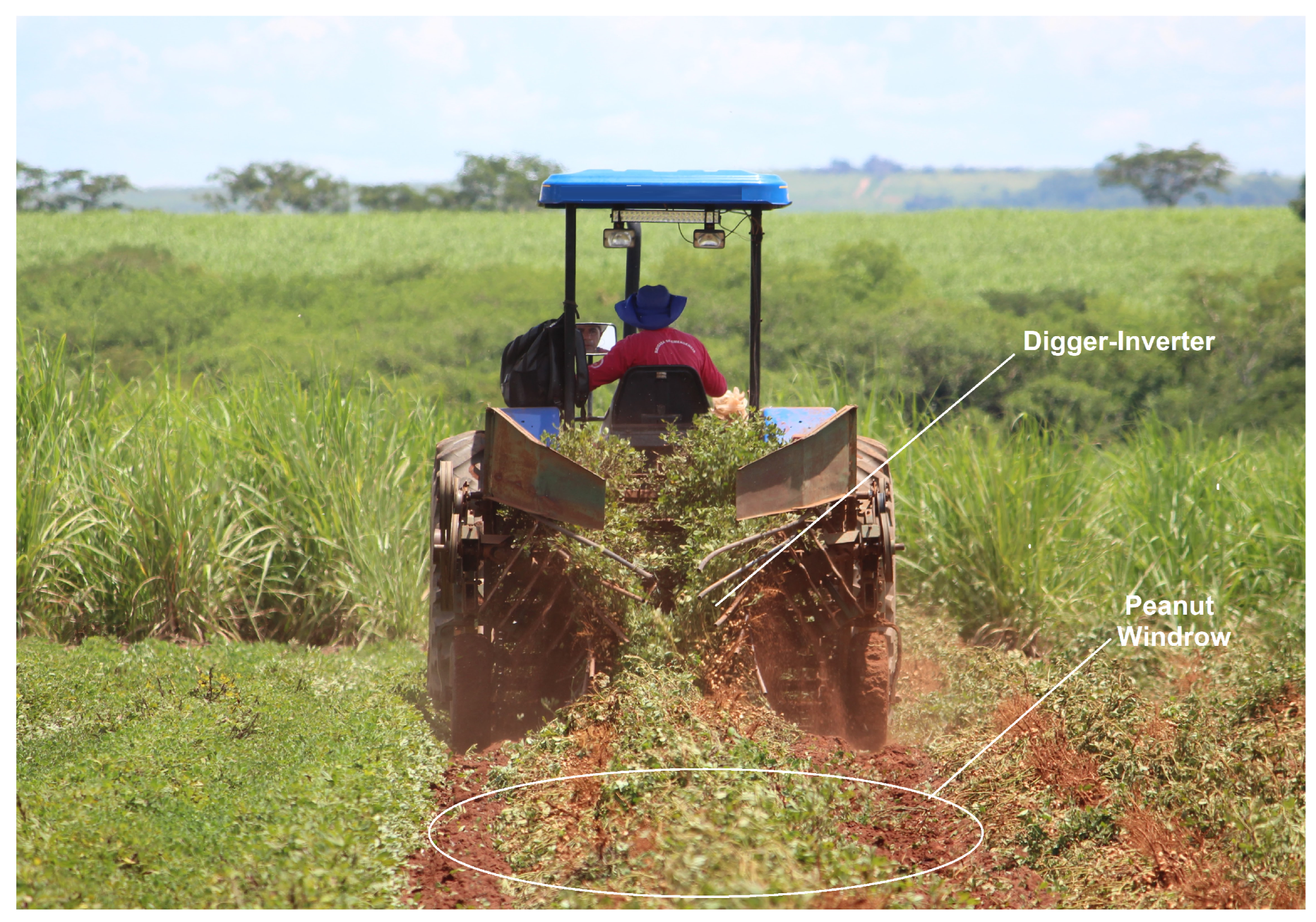
Finally, this article is organized as follows. Section 2 (Mechanized Harvesting and Losses in Peanut Cultivation) characterizes the problem, detailing aspects related to the harvesting process and the losses inherent to this process when carried out in a mechanized manner. In Section 3 (Materials and Methods), the proposed system is detailed, from image acquisition to the determination of the coordinates of the points that are part of the soil profile collected with the proposed sensor. In Section 4 (Results), the results obtained with the use of the proposed sensor in experiments involving measurements on the ground (real and not simulated measurements) and a comparison of the results with those obtained by the manual method (use of a profilometer) are presented. In Section 5 (Conclusions) the main conclusions regarding the obtained experimental results are presented, as well as a discussion regarding the validity of the proposed method.

2. Mechanized Harvesting and Losses in Peanut Cultivation

For mechanized peanut harvesting, the following two steps are necessary: digging and collecting. By using a machine called a digger–inverter (Figure 1), the processes of digging and windrowing are carried out simultaneously. At the front of the machine, there are two disks responsible for cutting the branches. Two cutting blades pull the plants out of the ground, and the guide rods direct them onto an elevating conveyor belt. From the top of the conveyor, the plants fall into the inversion system and are left on the ground, forming a windrow with the pods facing upwards and the foliage downwards, making it easier to dry the fruit. The equipment also has a vibration system to remove excess soil from the pods. The machine is driven by a medium-sized tractor (power class III). Figure 2 shows the windrowing process, forming the windrow.

To reduce losses inherent to the process, harvesting must be carried out in the shortest possible time. The monitoring of losses makes it possible to detect errors that occur during the harvesting process and, thus, minimize losses through corrective measures. Most losses in peanut production occur during the digging operation [34] and are due to the interaction of various factors related to both the crop (soil, time of digging, climate, crop health, development conditions, weeds and maturity) and the machinery used (design, adjustment, maintenance and speed) [17]. Analysis of the causes and effects that determine losses leads to improvements in the involved operations, contributing to the sustainability of the production chain.

Total Digging losses (TDLs) are related to Visible Digging Losses (VDLs) and Invisible Digging Losses (IDLs). The first correspond to the pods and grains that are deposited on the soil after the digging operation. The other losses (invisible losses) are losses related to the pods and grains found below the soil after the operation. Based on these parameters, the total digging losses can be determined using Equation (1). The unit used is kg per hectare (kg/ha).

$$\begin{array}{c}\hfill TDL=VDL+IDL\end{array}$$

(1)

Total visible losses correspond to the pods and grains found on the surface of the soil after the harvesting operation. The methodology commonly used to assess quantitative losses consists of collecting pods and grains at sampling points in the area where peanuts have been dug/inverted and subsequently harvested. For this purpose, a metal frame is used to delimit the sampling area to be evaluated. The pods and grains found on the surface of the ground and contained inside the frame are counted as visible losses during digging. At the same sampling point, the soil is removed and sieved. The pods and seeds removed from the soil comprise the invisible losses during digging. Experimental work in the area has reported total digging losses of around 37% of actual productivity, corresponding to losses of more than 1 ton per hectare.

Figure 3 illustrates the collection procedures.

Evaluating harvesting performance also involves measuring the dimensions of the bed formed after digging. Estimating the geometry of the windrow makes it possible to maintain the feed rate of the harvester (the machine used after the digging/inversion operation), contributing to efficient action. The dimensions of the windrow are usually determined using rudimentary equipment, where the width and height of the windrow are measured using a tape measure and a graduated steel bar, respectively. Profilometers are also used in conjunction with digital cameras, as shown in Figure 4. The automation of this process of estimating the dimensions of the windrow can be used to generate estimates of losses in the production process.

In an important experimental work [28], harvesting losses were correlated with the height of the peanut windrow generated during the digging/inversion operation. The authors found that the height of the windrow and the visible losses in the harvesting process showed a positive correlation. Therefore, it was possible to state that the greater the height of the windrow, the greater the visible losses in the harvesting process. Figure 5 and Figure 6 below show the obtained experimental results.

The correlation between the height of the windrow and the amount of visible losses is clear. Based on this survey, this paper presents a technique for evaluating the profile of the windrow formed after digging. The results obtained with this technique can be used to adjust its operating height of the digging machine, modifying the height of the formed windrow in real time and, consequently, reducing losses. This technique is described in the following sections.

3. Materials and Methods

The methodology used in this study is shown in the block diagram in Figure 7. A laser beam with a line profile is projected onto the surface of the windrow and captured by a monocular camera. The processed images are used to estimate the three-dimensional coordinates of the points of incidence of the beam on the windrow. By computing the coordinates of these points, it is possible to create a 3D profile of the windrow. In the image acquisition stage, a subtraction strategy is used between a pair of consecutive images in order to highlight the projection of the beam on the image. In the next step, an optimized segmentation algorithm is used to separate the beam projected onto the image. Subsequently, in the beam detection stage, specific characteristics of the beam are used to identify it from the segmented image. In the last stage, a triangulation model is used to obtain a point cloud from the coordinates of the beam projection on the image. These steps are shown in detail below.

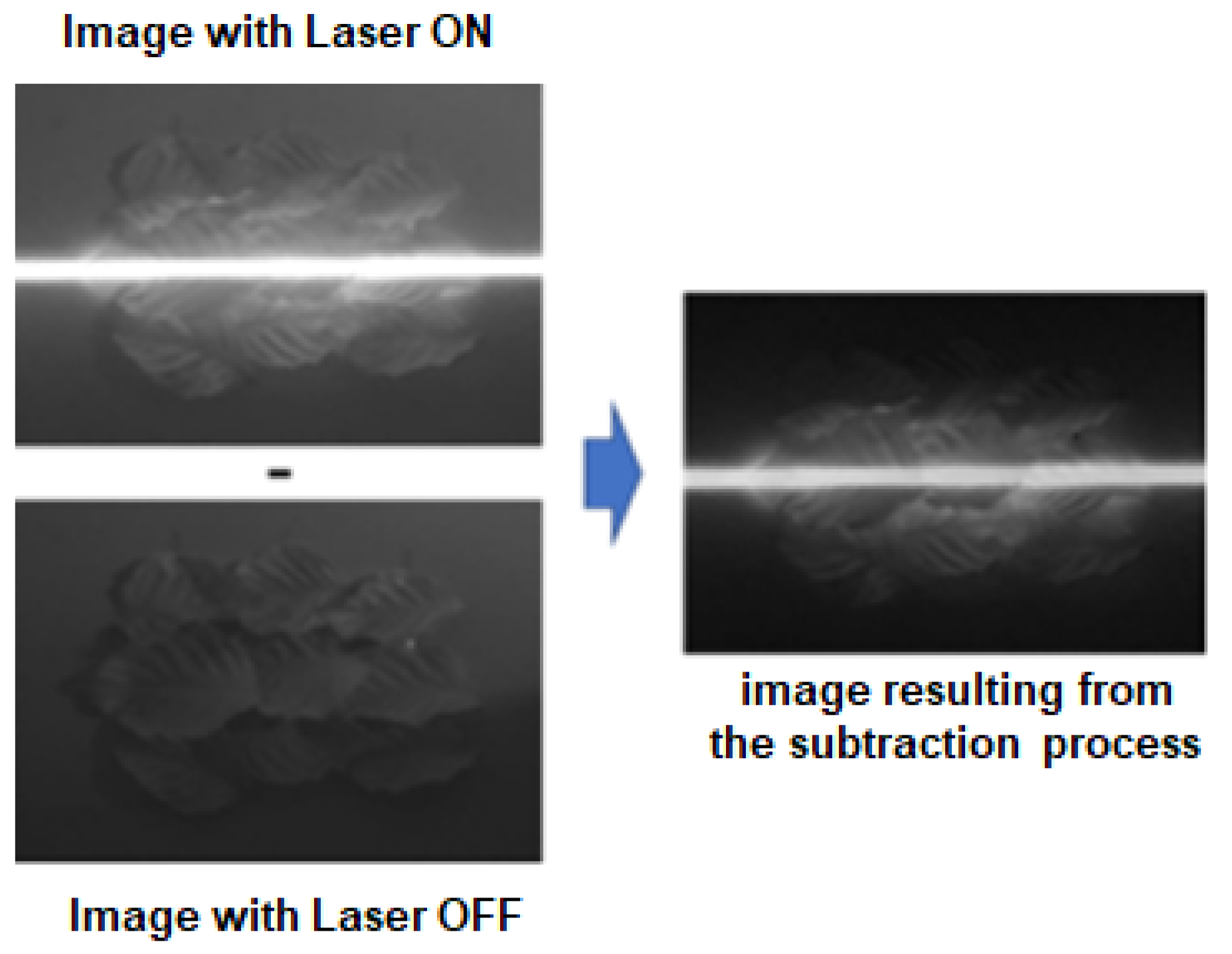
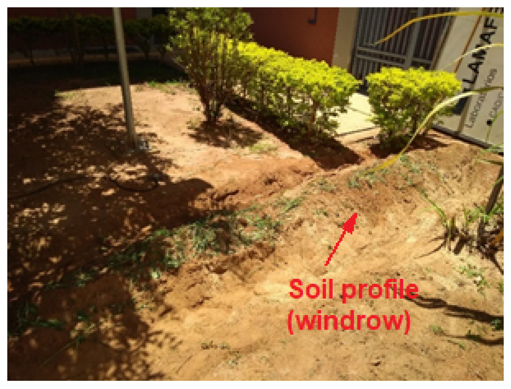
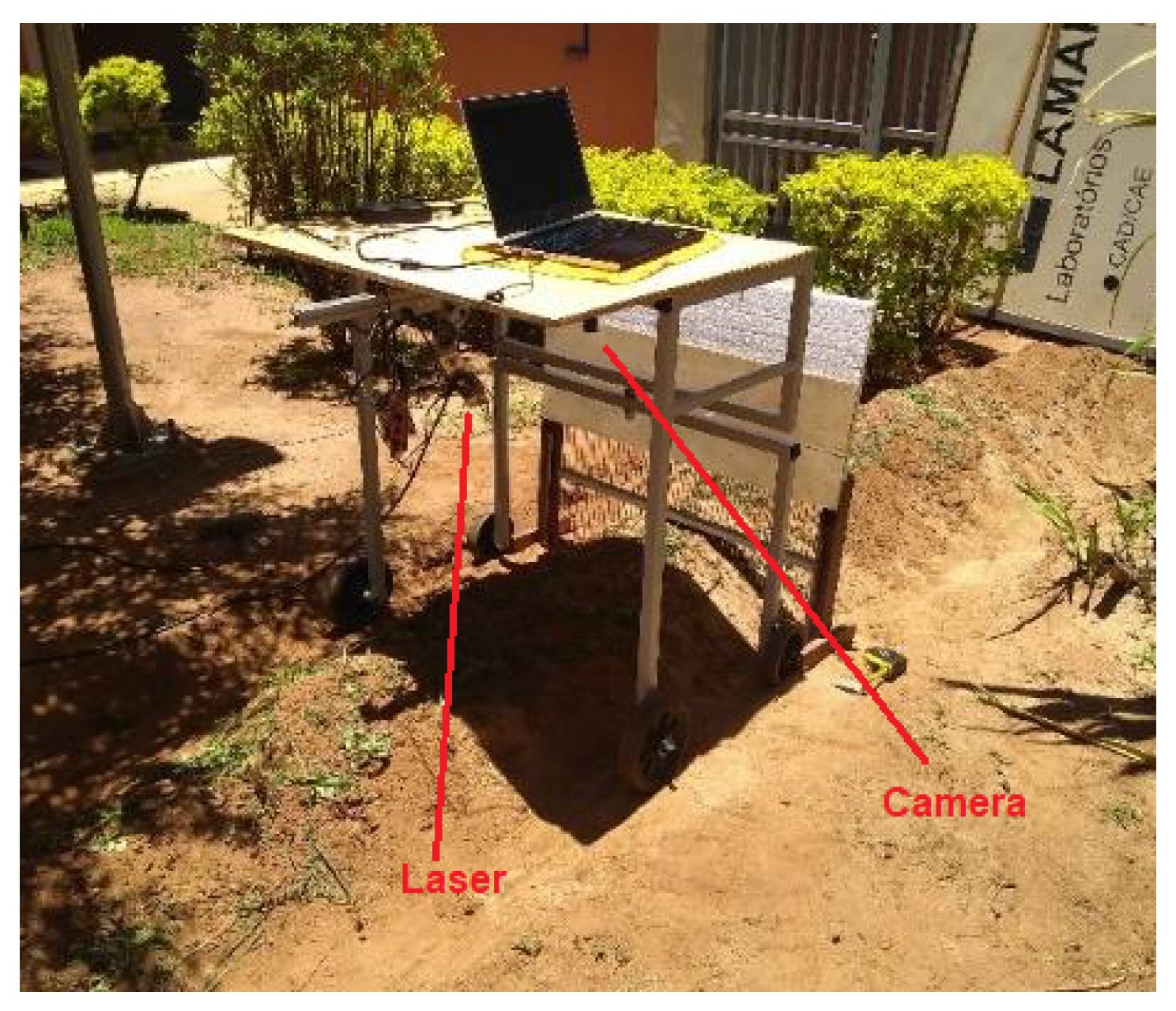
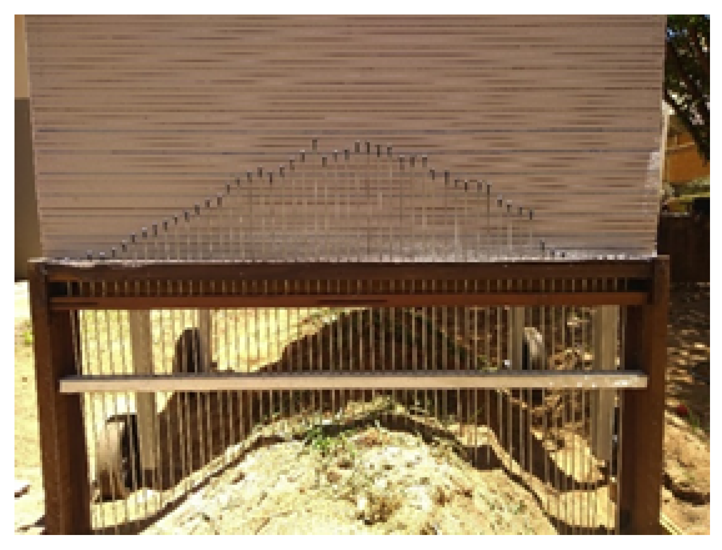
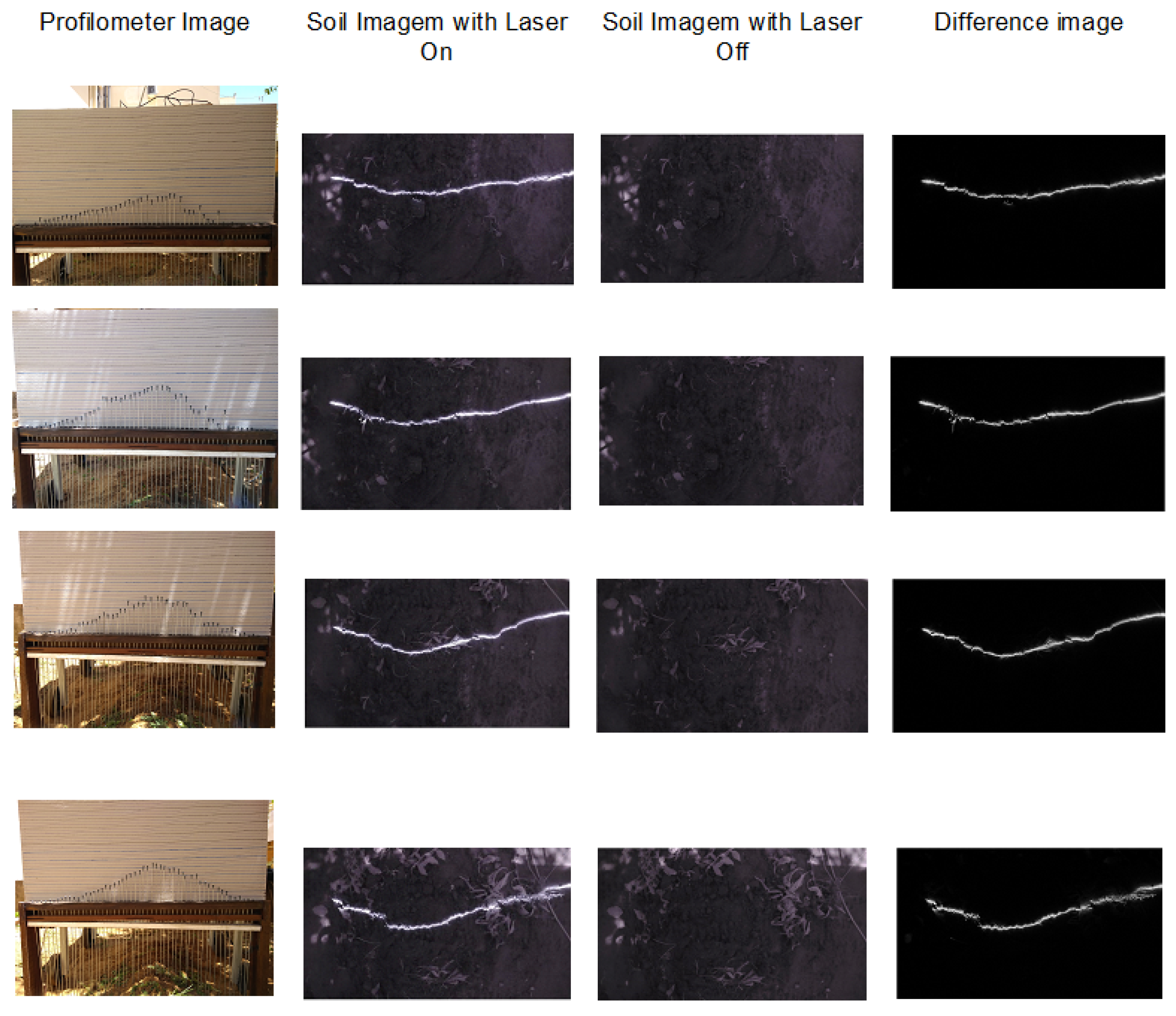
3.1. Acquisition of Images

The image subtraction strategy was used, which consists of sequentially acquiring two images—one with the laser on and the other with the laser off. With the projection of the beam present in only one of the images, the subtraction process produces an image in which the beam is highlighted in intensity, as shown in Figure 8.

Although this strategy leads to a better result in image segmentation, it is necessary to impose a minimum movement of the device in the interval between capturing the pair of images. In this way, the time involved in this process becomes a relevant variable. Intervals that are too long can make it difficult to acquire images of the same scene, and on the other hand, shorter intervals may be insufficient to correctly activate the laser and acquire the beam projected onto the surface. In this study, an experiment was carried out to characterize the transient of the laser and camera set, allowing the ideal interval for sampling in pairs to be estimated. This interval was defined experimentally as 70 ms. For this purpose, two acquisition sequences were defined, as shown in Figure 9. In the first sequence, acquisition begins with the laser switched on. The laser is then switched off, and the devices are left to settle for the second acquisition. In the second sequence, the first image is acquired with the laser switched off, and the laser is switched on after the settling-in time to carry out the second acquisition.

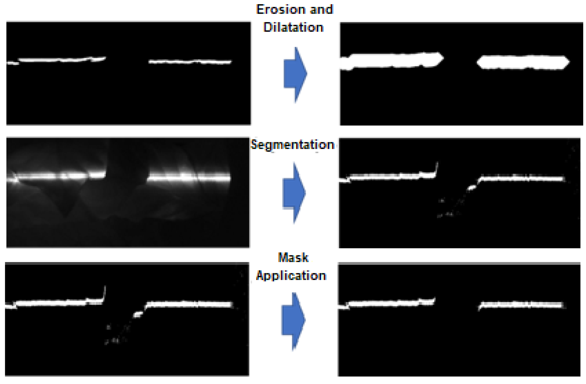
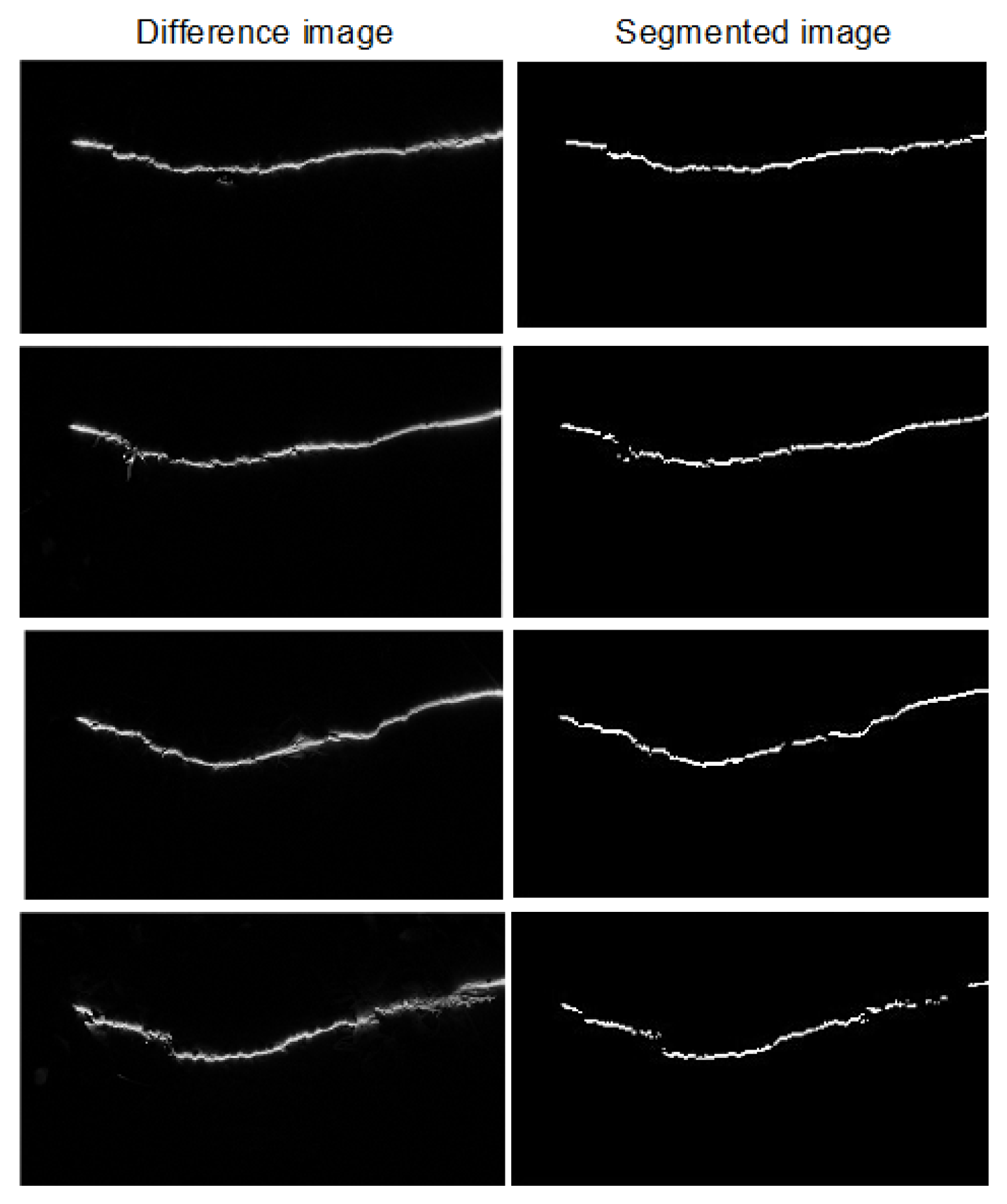
3.2. Segmentation

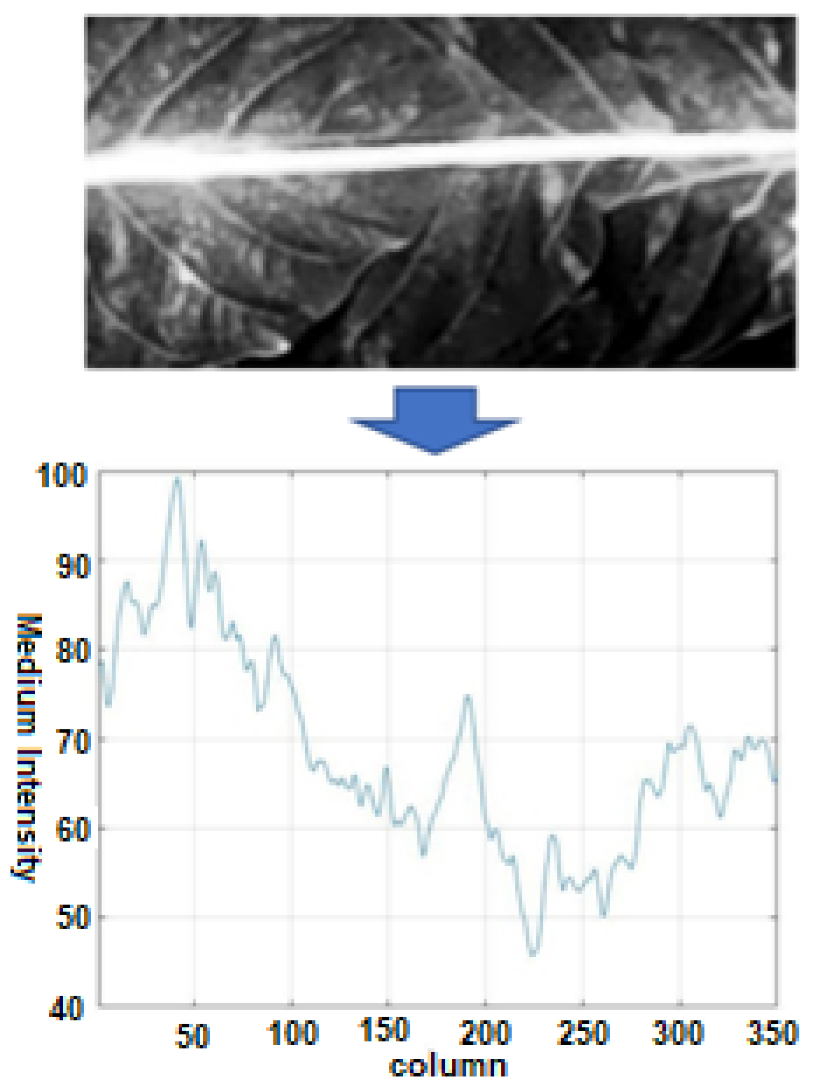
3.2.1. Adaptive Segmentation

In the image segmentation process, the step called optimized adaptive segmentation carries out the segmentation process using the average thickness expected for the beam projection onto the image, measured in number of pixels, and using the spatial information in which the beam is distributed horizontally in the image. The adopted strategy showed very satisfactory results in segmenting the beam. However, a significant number of false positives were obtained in regions far from the beam in which the image shows little contrast. The adopted solution was to include a step to identify these regions, then remove them from the segmentation result. In addition, morphological operation steps were included to improve the results. As the laser beam is arranged horizontally across the image, adaptive segmentation by region is carried out considering each column of the image. Thus, for each column, the average intensity of the pixels is initially calculated as illustrated in the graph in Figure 10. In this figure, the horizontal coordinate of the image is represented on the horizontal axis, and the average intensity of the pixels in the respective column is represented on the vertical axis.

Considering that the beam has an intensity that overlaps regionally with the background, the optimal threshold for local segmentation of the beam in the column is expected to be in the range between the integer ($m_i$) closest to the average value for the column intensity and the maximum value allowed in the image (usually 255). To estimate the ideal threshold ($L_i$), for each possible threshold (Li,k), the number of pixels with a value greater than the threshold is calculated, as represented by Ni,k. Since E is an expectation for the beam thickness, the optimal threshold is expected to have the sum (Ni,k) closest to E. Equation (2) formalizes the process for calculating the threshold for each image column. In addition to expecting the optimal threshold to have a number of pixels similar to the beam width, it is also expected that the pixels will be preferentially concentrated in their respective region of incidence. For this reason, the Ci,k term was added to the equation to penalize possible Li,k thresholds with a greater number of related elements. The calculation of the Ci,k term is shown in Equation (3), where Eci,k is the number of connected elements calculated for each column (i) and value (k). The constant that multiplies the Ci,k term in Equation (2) was established empirically through experiments.

$$\begin{array}{c}\hfill L_i=min\left(\right|N_{i,k})-E|+8C^{i,k},kϵ\mathbb{N}:m_i<k<255\end{array}$$

(2)

$$\begin{array}{c}\hfill C_{i,k}=\left\{\begin{array}{ccc}{E}_{C_{i,k}}-1,& E_{C_{i,k}}\ge 1& \\ 0,& E_{C_{i,k}}<1& \end{array}\right.\end{array}$$

(3)

The first step in the process of segmenting regions with low contrast was to use the Prewitt filter to emphasize the horizontal edges of the image. Subsequently, an averaging filter was applied using a mask with dimensions of 5 × 12. This strategy made it possible to attenuate scattered elements and preserve the horizontal edges. The result is shown in Figure 11.

3.2.2. Detection and Removal of Regions without Contrast

Regions with an intensity below the 20% threshold after filtering were classified as having insufficient contrast and were marked as background in the thresholding process, as shown in Figure 12.

The threshold used was established empirically. In the next step, the morphological erosion operation was applied with a structuring element with dimensions of 3 × 3 in order to remove small elements resulting from noise in the image. Finally, the dilation operation was carried out using a diamond-shaped structuring element with a radius of 20 pixels. The appropriate intensity of the beam, according to the lighting conditions, results in sharp edges in the respective region. Considering that the expansion through dilation is greater than the thickness of the beam, it is expected that it will be contained within the segmented image obtained in this process. In this way, the obtained result is used as a mask after the adaptive beam segmentation process. Figure 13 shows the process.

The image used in the examples consists of overlapping leaves with a difference in depth sufficient to cause beam occlusion in the center of the image and close to the edge on the right-hand side, making it possible to clarify the purpose of this strategy. The beam occlusion regions do not meet the conditions assumed when the adaptive segmentation algorithm was developed, resulting in an incorrect threshold for the respective columns. Therefore, obtaining a mask to separate the low-contrast region eliminates false positives due to the occlusion problem.

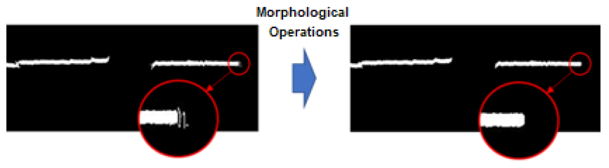
3.2.3. Morphological Operations

In the final stage of the segmentation process, the morphological opening operation is used, followed by the closing operation, with the aim of perfecting the segmented image. The used structuring elements are diamond-shaped, with the radius of the element in the first operation equal to 2 pixels and that in the second equal to 5 pixels. Figure 14 illustrates the obtained result, showing the effect of the morphological operations.

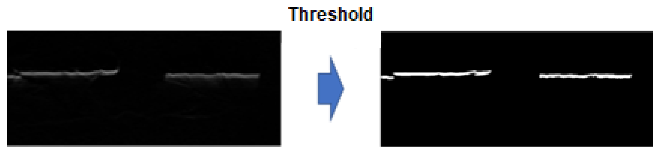
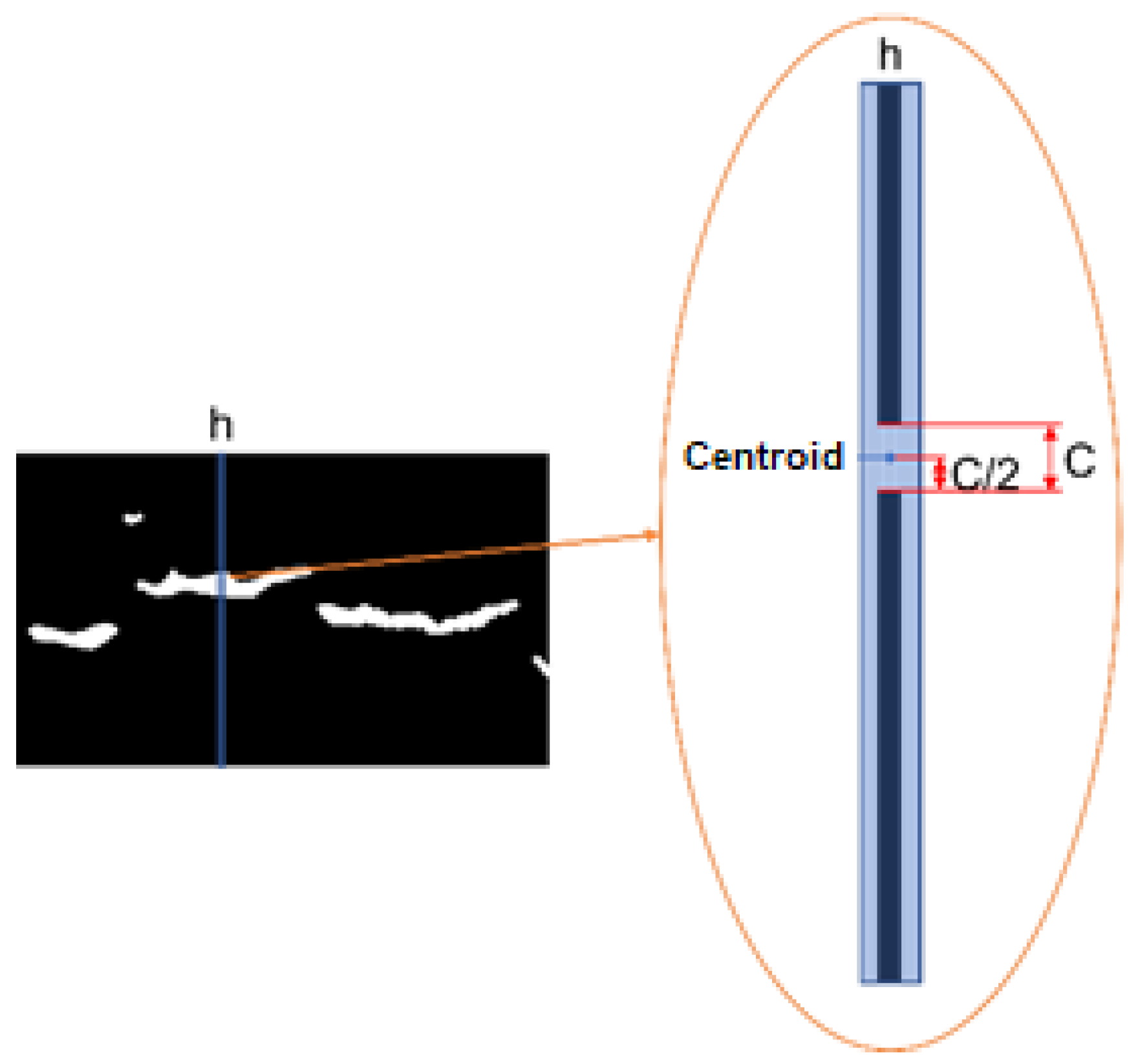
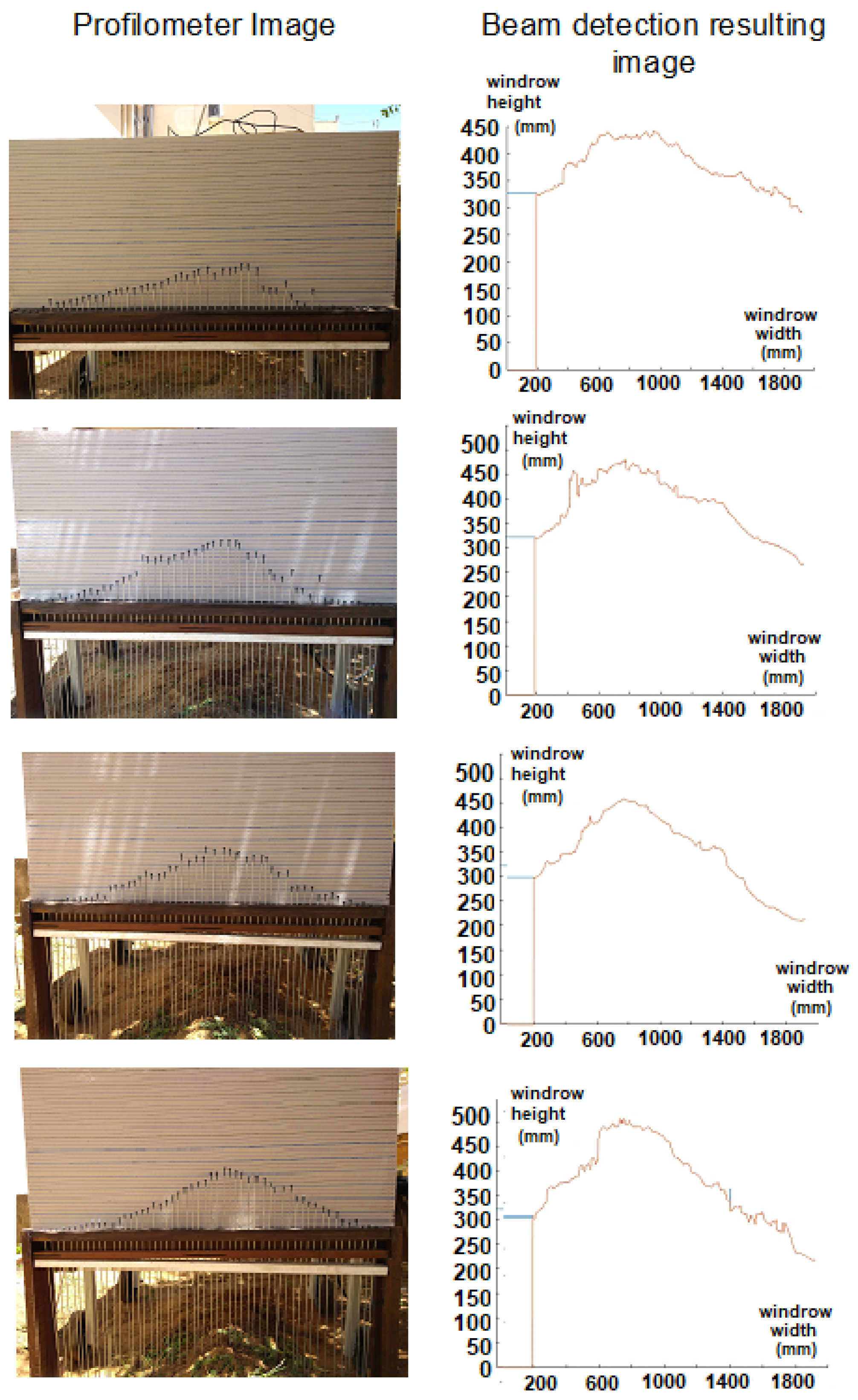
3.3. Beam Detection

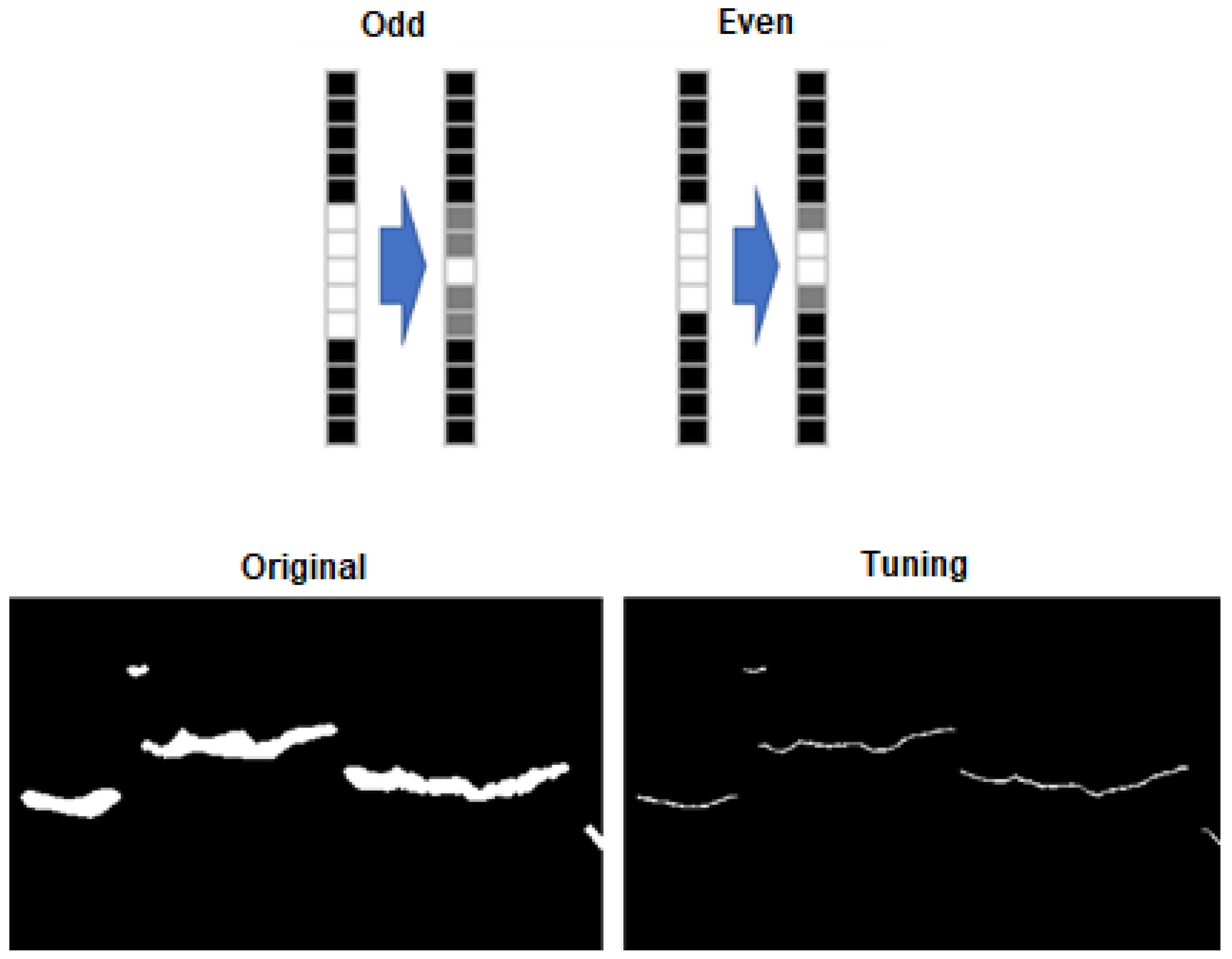
3.3.1. Column Thinning

The proposed approach to the image thinning process uses the previously known characteristic of the image in which the beam must be found to be positioned horizontally across the image. The result of the thinning process using the traditional method based on morphological operations is illustrated in Figure 15.

The result obtained using this method produces bifurcations at the ends and along each segment, which can cause ambiguities in the three-dimensional reconstruction process. The strategy adopted to carry out the thinning process consists of separately searching each column (h) of the image for related elements, then calculating the centroid of the elements, as illustrated in Figure 16.

For connected elements of odd size, the centroid can be obtained by averaging, and for elements of even size, the centroid is defined as the two central pixels of the element. This strategy makes it possible, later in the dimensionality transformation stage, to identify the pixel’s position as an average between the two central pixels, allowing for minimization of quantization errors in the triangulation process. The strategy for representing the centroid of the connected elements and the result of the thinning process are illustrated in Figure 17.

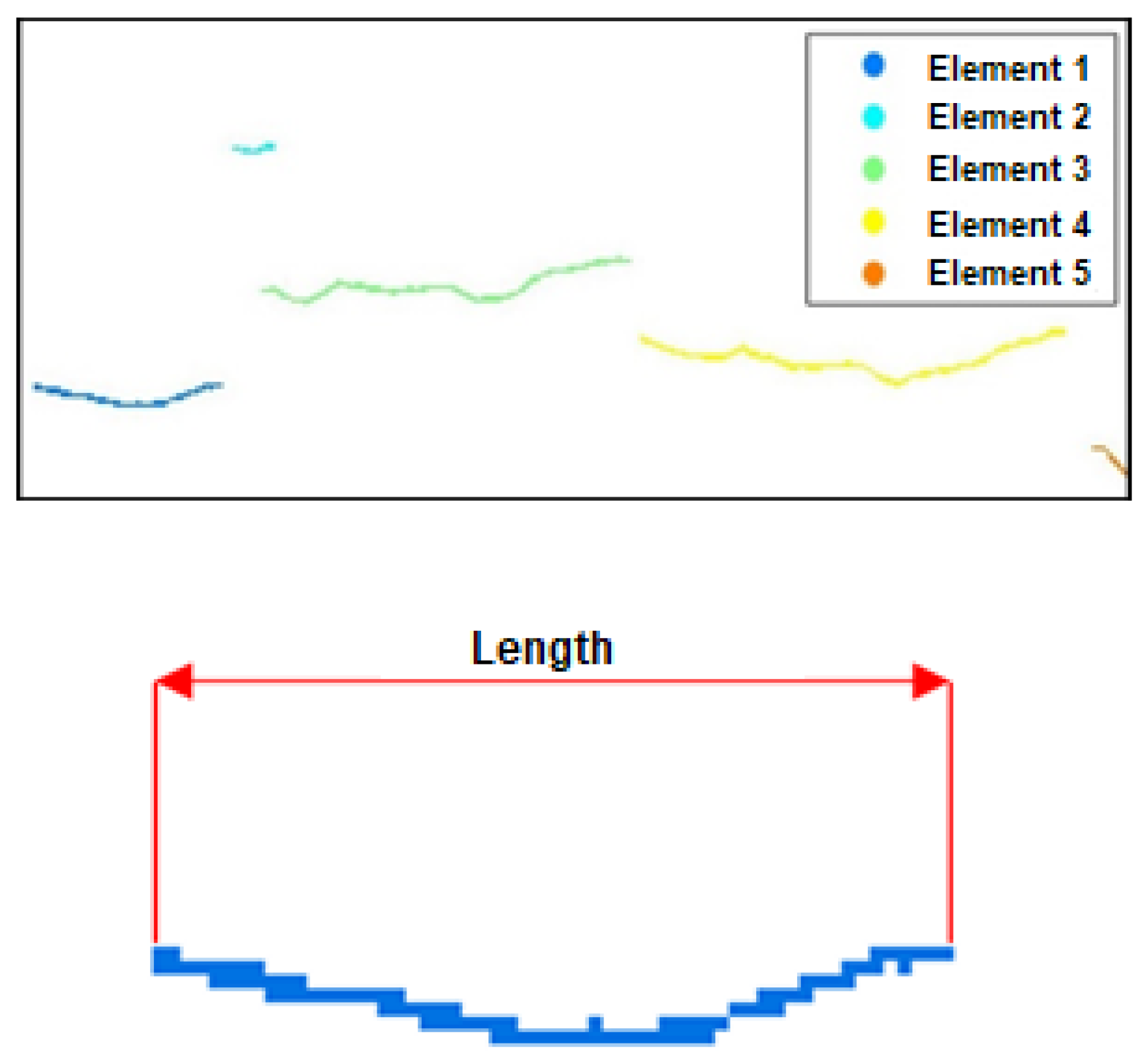
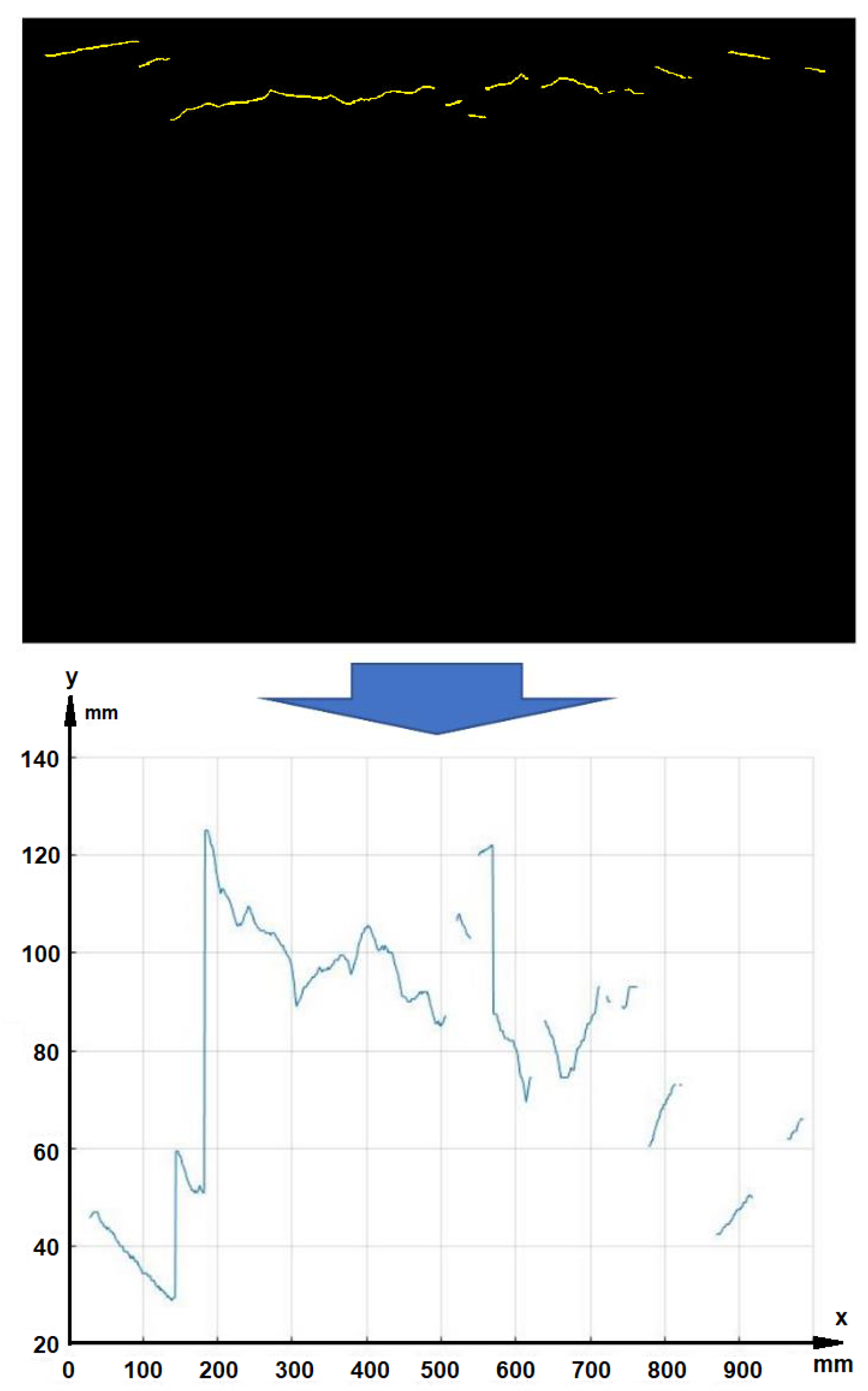
3.3.2. Extraction of Connected Elements

At this stage, the connected elements in the sharpened image are extracted and enumerated using connectivity-8. For each element, the length is calculated considering only the coordinates. Figure 18 shows the result obtained in this process.

3.3.3. Vertical Overlap Removal

Knowing the characteristic of the beam that must be projected along the horizontal axis of the image, the vertical overlap of elements in the image is considered a flaw that can be associated with laser reflections on the incident surface. Therefore, the next stage of the beam extraction algorithm consists of the process of removing vertically overlapping elements. The adopted strategy consists of first eliminating the overlapping pixels while retaining the element with the longest length. After this operation, the length of each element is recalculated to eliminate the elements considered to be outliers. In the example illustrated in Figure 19, the connected element highlighted in red was eliminated because its final length was less than 50% of its initial length.

The adopted criterion consists of removing elements whose final lengths are less than a threshold and eliminating elements whose final lengths are less than a certain fraction of the length before the process of eliminating overlapping pixels. Although these parameters can be adjusted according to the specific characteristics of the local culture, in preliminary tests, the parameters were set at 10 for the minimum length and 50% for the maximum reduction allowed for an element. In the illustrated example, the connected element highlighted in red was eliminated because its final length was less than 50% of the initial length.

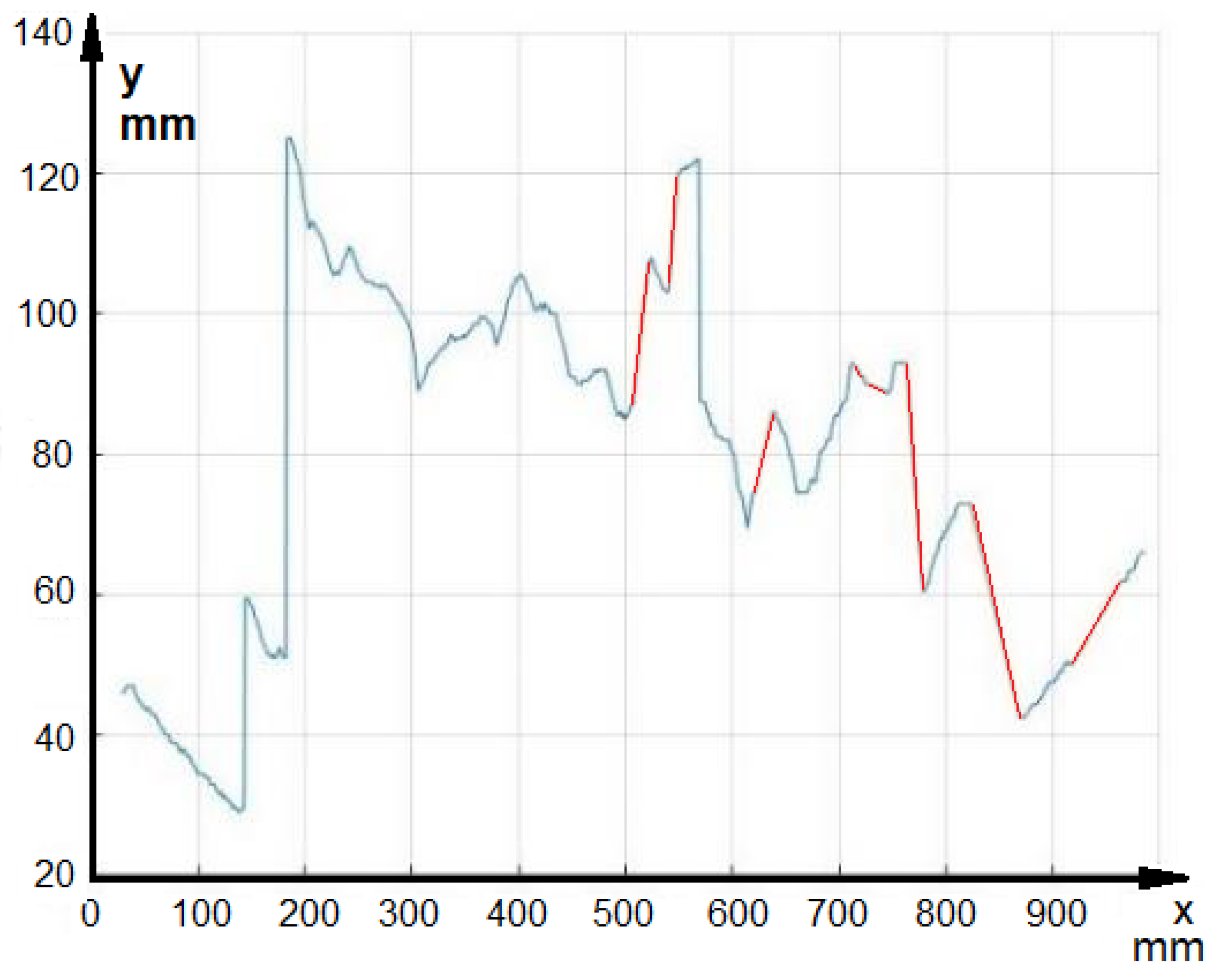
3.3.4. Interpolation

At this stage, the image representing the laser beam on the windrow is a binary image in which there is only one pixel with a value of “1” in each column. Before being submitted to a triangulation process, this image must undergo a dimensionality transformation process, followed by an interpolation process. In the dimensionality transformation, a function (g(x)) is used to transform the vertical coordinate (y) of a pixel (p) in the image, which is defined by f(x,y), according to Equation (4).

$$\begin{array}{c}\hfill p=f(x,y)\Rightarrow y=g\left(x\right)\end{array}$$

(4)

In this equation, the left side shows the value of any pixel (p) using the function f(x,y). On the right side, the result of the transformation is shown, which obtains a function (g(x)) for the vertical coordinate (y). Figure 20 shows an example of the process.

In the interpolation process, for columns containing two adjacent pixels, the y-coordinate value is calculated using the average of the two pixels, obtaining a spatial resolution of 0.5 pixels for the vertical coordinate. For the region of the image in which there are no “1” pixels in any column, the y value is obtained by linear interpolation. The “0” pixels at the ends of the x axis are kept as zero in the interpolation process. This feature allows these pixels to be excluded in the reconstruction process. Thus, the beginning and end of the beam correspond to the first pixels with values of “1” at the ends of the axis. Figure 21 shows the result after the interpolation process. The segments obtained through interpolation are highlighted in red in the graph.

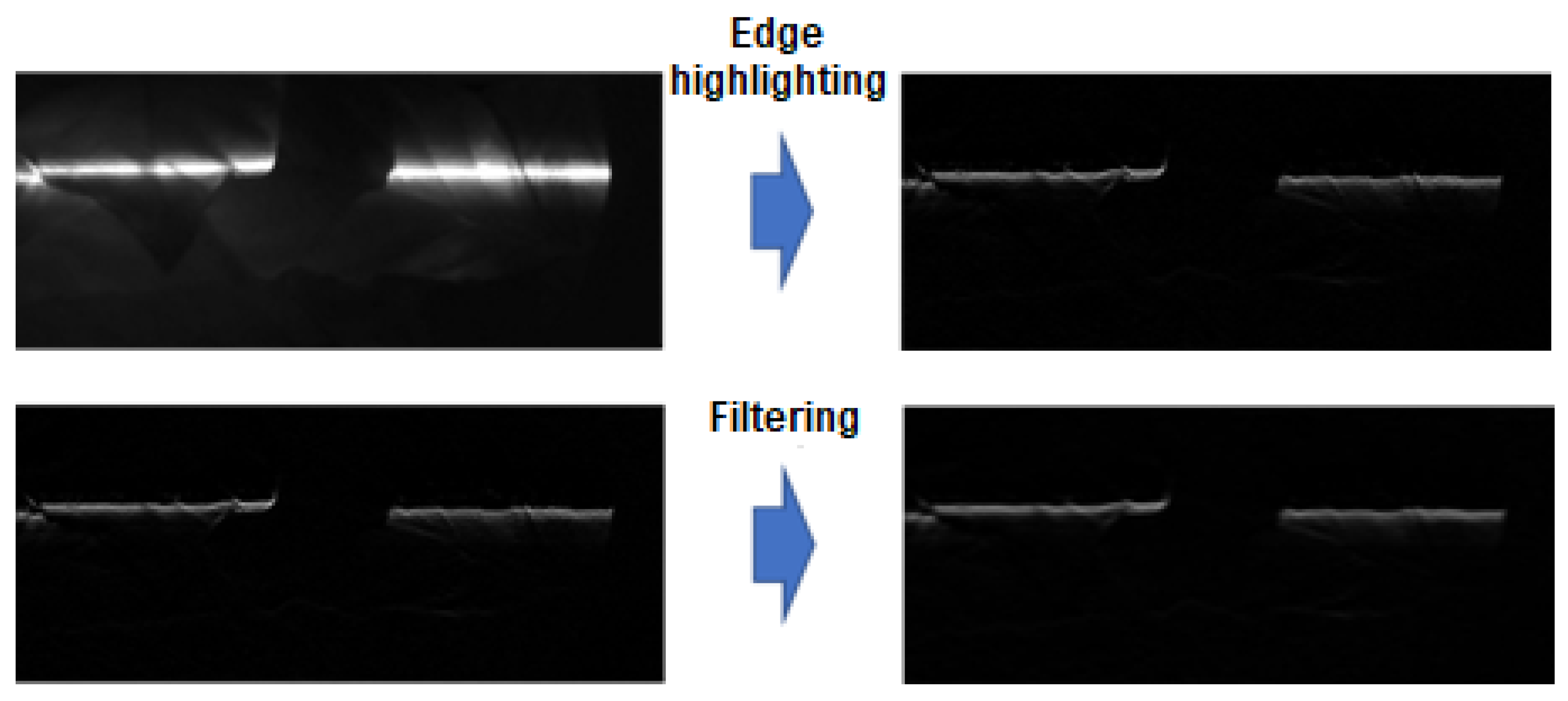
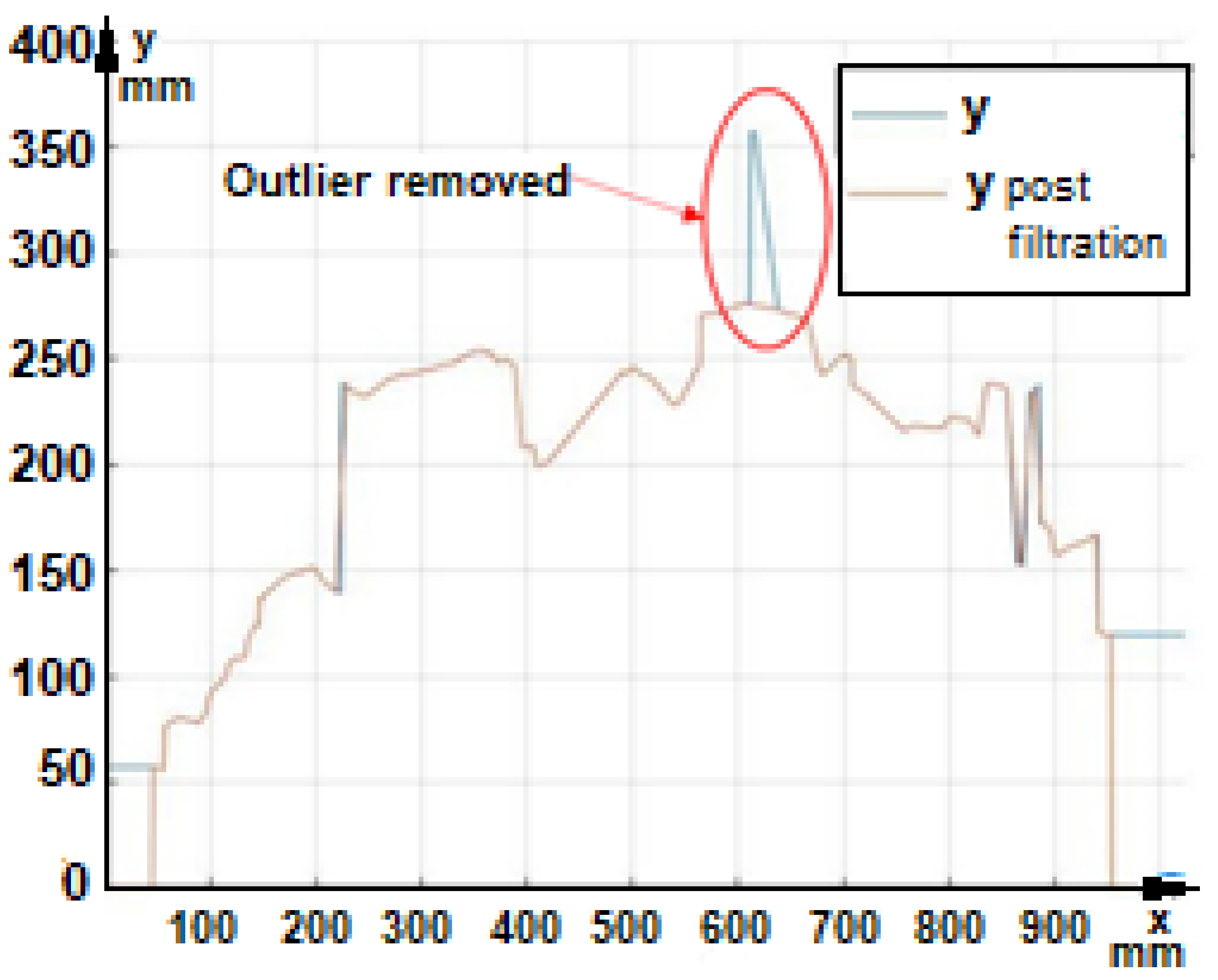
3.3.5. Filtering

In the filtering stage, digital signal processing techniques are used to remove elements that are considered outliers according to the previously adopted criteria, as shown in Figure 22.

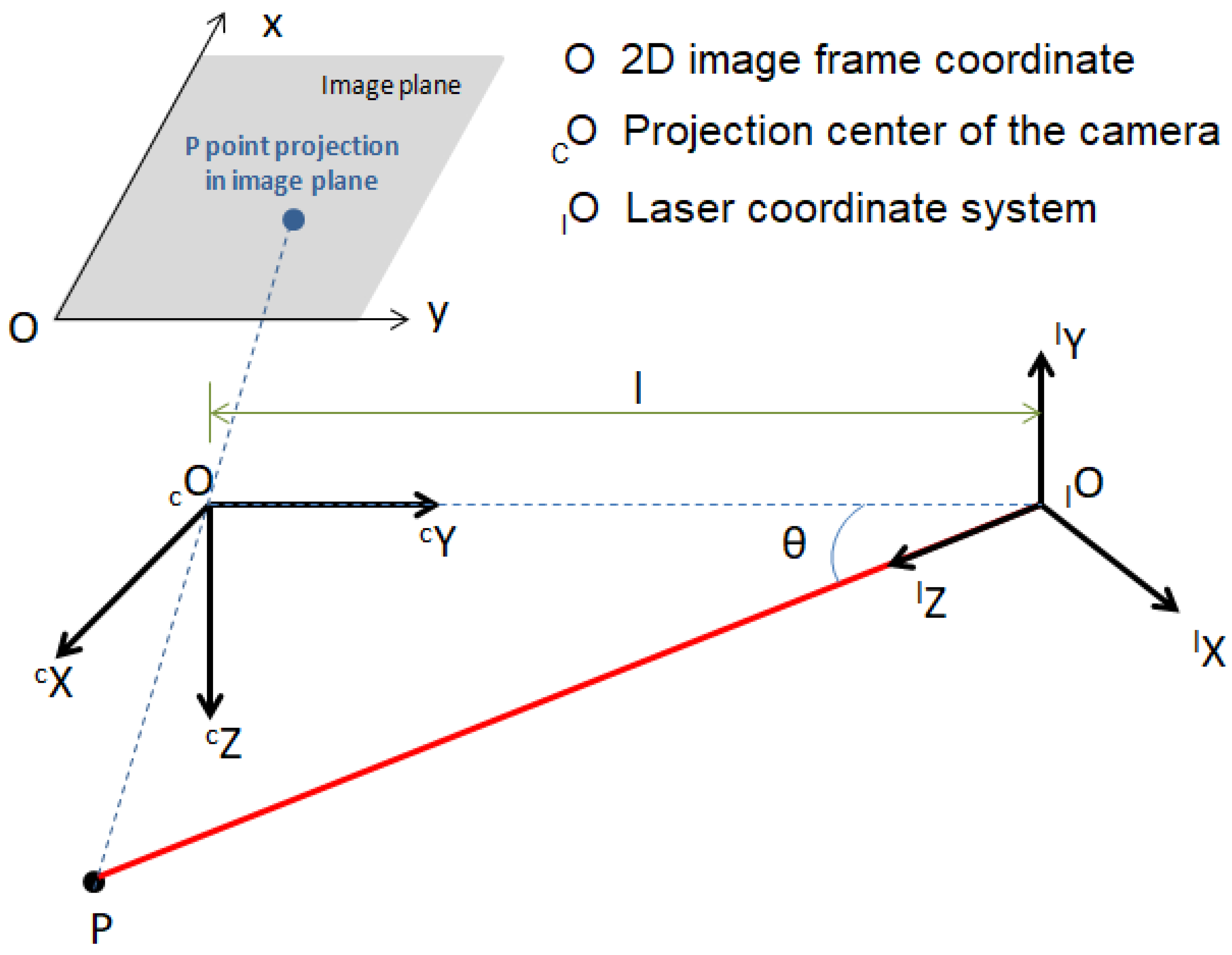
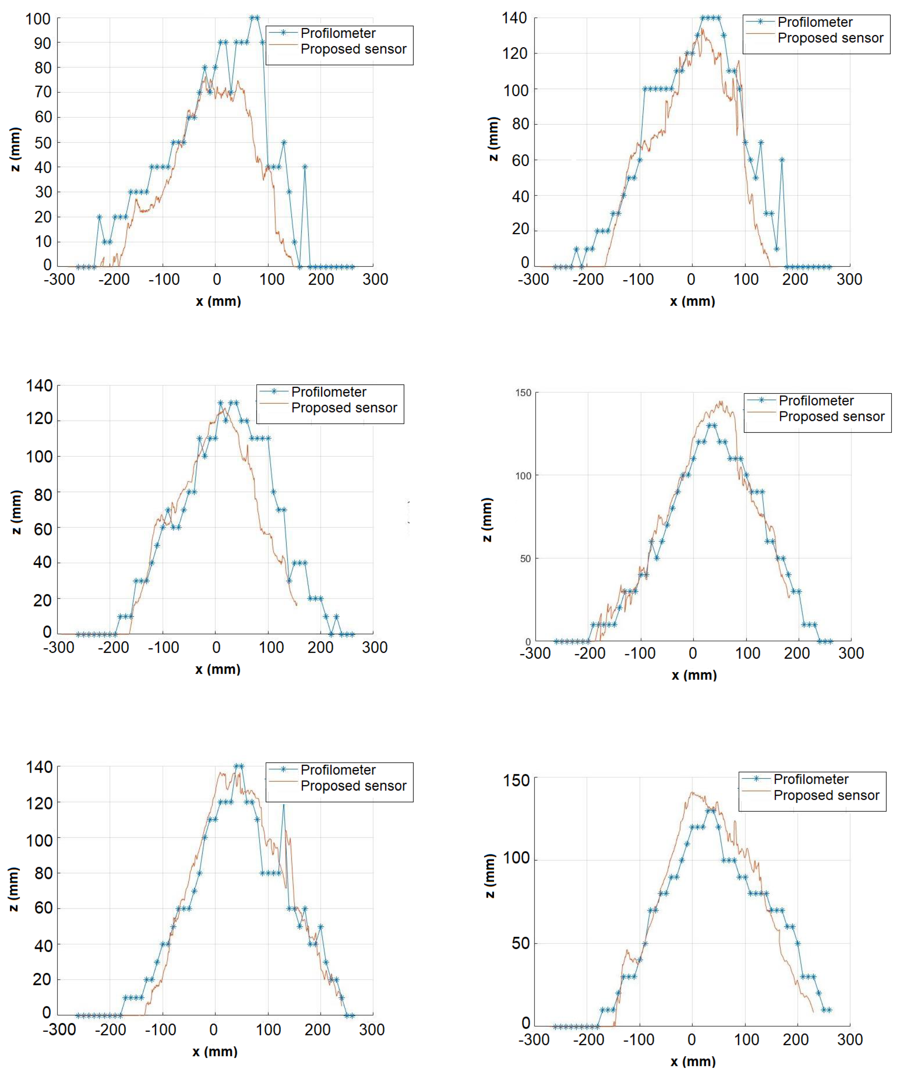
3.4. Triangulation

In the triangulation stage, the coordinates of the beam are used to perform the three-dimensional reconstruction of the scene, then georeference the measurements using the positioning estimates of a sensor fusion system. To calculate the three-dimensional coordinates of the windrow profile, triangulation was used between the beam emitted by the laser and its projection on the image. The triangulation scheme used for the reconstruction process in the next stage is shown in Figure 23. The terms x and y are the image coordinates in the camera’s projection plane; ^cX, ^cY and ^cZ are the three-dimensional coordinates considering the camera coordinate system; and ^lX, ^lY and ^lZ are the coordinates in the laser system. The geometric parameters are the distance (d) between the camera and laser coordinate systems, and the angle is $\theta$.

The image coordinates in pixels can be transformed into the coordinate system of the camera’s projection plane using Equations (5) and (6). The coordinates of a point in the image, in pixels, are given by $O_x$ and $O_y$. The effective pixel size is given by $S_x$ and $S_x$. The image coordinates, in pixels, are given by $x_{im}$ and $y_{im}$.

$$\begin{array}{c}\hfill x=-(x_{im}-O_x)S_x\end{array}$$

(5)

$$\begin{array}{c}\hfill y=-(y_{im}-O_y)S_y\end{array}$$

(6)

The transformation process from the laser coordinate system to the camera coordinate system is shown in Equation (7). The terms ^cP and ^lP represent any point in the camera and laser coordinate system, respectively. The vector ^cT_l consists of the laser position for the camera coordinate system, as defined using Equation (8). The rotation matrix (${}_l{}^c\mathrm{R}$) relates the orientation of the coordinate systems, as defined using Equation (9).

$${}^c\mathrm{P}={}_l{}^c\mathrm{R}+{}^c\mathrm{T}_l$$

(7)

$${}^c\mathrm{T}_l=\left[\begin{array}{c}0\\ -d\\ 0\end{array}\right]$$

(8)

$$\begin{array}{c}\hfill {}_l{}^c\mathrm{R}=\left|\begin{array}{ccc}1& 0& 0\\ 0& sen\left(\theta \right)& cos\left(\theta \right)\\ 0& -cos\left(\theta \right)& sen\left(\theta \right)\end{array}\right|\end{array}$$

(9)

Using the definition of the rotation matrix (${}_l{}^c\mathrm{R}$) and the translation vector (${}^c\mathrm{T}_l$), Equation (7) can be rewritten as shown in Equation (10).

$$\begin{array}{c}\hfill {}^c\mathrm{P}=\left[\begin{array}{c}{}^c\mathrm{X}\\ {}^c\mathrm{Y}\\ {}^c\mathrm{Z}\end{array}\right]=\left[\begin{array}{c}{}^l\mathrm{X}\\ {}^l\mathrm{Y}sen\left(\theta \right)+{}^l\mathrm{Z}cos\left(\theta \right)-d\\ -{}^l\mathrm{Y}cos\left(\theta \right)+{}^l\mathrm{Z}sen\left(\theta \right)\end{array}\right]\end{array}$$

(10)

As shown in the representation of the triangulation model in Figure 23, the coordinate in the laser system (${}^l\mathrm{Y}$) for any point of incidence of the beam is zero. Equations (11)–(13) are obtained by applying this constraint to Equation (10).

$$\begin{array}{c}\hfill {}^c\mathrm{X}={}^l\mathrm{X}\end{array}$$

(11)

$$\begin{array}{c}\hfill {}^c\mathrm{Y}={}^l\mathrm{Z}cos\left(\theta \right)-d\end{array}$$

(12)

$$\begin{array}{c}\hfill {}^c\mathrm{Z}={}^l\mathrm{Z}sen\left(\theta \right)\end{array}$$

(13)

To obtain an independent equation in the camera system, the ${}^l\mathrm{Z}$ term was isolated from Equation (12) and substituted into Equation (11). The result is shown in Equation (14).

$$\begin{array}{c}\hfill {}^c\mathrm{Y}={}^c\mathrm{Z}cot\left(\theta \right)-d\end{array}$$

(14)

The perspective projection model relates the camera coordinate system to the image projection plane system, as shown in Equations (15) and (16). The $f_x$ and $f_y$ parameters correspond to the focal length of the camera.

$$\begin{array}{c}\hfill x=f_x{\displaystyle \frac{{}^c\mathrm{X}}{{}^c\mathrm{Z}}}\end{array}$$

(15)

$$\begin{array}{c}\hfill y=f_y{\displaystyle \frac{{}^c\mathrm{Y}}{{}^c\mathrm{Z}}}\end{array}$$

(16)

Substituting the ${}^c\mathrm{Y}$ term from Equation (15) into Equation (13) gives the equation for the ${}^c\mathrm{Z}$ coordinate as a function of the y coordinate of the image projection plane, as shown in Equation (17).

$$\begin{array}{c}\hfill {}^c\mathrm{Z}={\displaystyle \frac{d}{f_{y}cot\left(\theta \right)-y}}{f}_y\end{array}$$

(17)

The equation for the ${}^c\mathrm{Y}$ component was obtained by substituting the ${}^c\mathrm{z}$ term from Equation (16) into Equation (17), as shown in Equation (18).

$$\begin{array}{c}\hfill {}^c\mathrm{Y}={\displaystyle \frac{d}{f_{y}cot\left(\theta \right)-y}}y\end{array}$$

(18)

To find the equation of the last component (${}^c\mathrm{X}$), the ${}^c\mathrm{Z}$ term was substituted from Equation (15) into Equation (17), as shown in Equation (19).

$$\begin{array}{c}\hfill {}^c\mathrm{X}={\displaystyle \frac{d}{f_{y}cot\left(\theta \right)-y}}x{\displaystyle \frac{f_y}{f_x}}\end{array}$$

(19)

The equations relating the image projection plane to the camera coordinate system can be rewritten in matrix form according to Equation (20).

$$\begin{array}{c}\hfill {}^c\mathrm{P}={\displaystyle \frac{d}{f_{y}cot\left(\theta \right)-y}}\left[\begin{array}{c}x{\displaystyle \frac{f_y}{f_x}}\\ y\\ f_y\end{array}\right]\end{array}$$

(20)

Since the intrinsic camera parameters ($f_x$, $f_y$, $S_x$ and $S_y$) are linearly dependent, the calibration process obtains the focal length expressed in the effective pixel size, as shown in Equations (21) and (22). Thus, Equation (23) is the equation used for the reconstruction process.

$$\begin{array}{c}\hfill f_{x,s}={\displaystyle \frac{f_x}{S_x}}\end{array}$$

(21)

$$\begin{array}{c}\hfill f_{y,s}={\displaystyle \frac{f_y}{S_y}}\end{array}$$

(22)

$$\begin{array}{c}\hfill {}^c\mathrm{P}={\displaystyle \frac{d}{f_{y,s}cot\left(\theta \right)+(y_{im}-O_x)}}\left[\begin{array}{c}(O_y-x_{im}){\displaystyle \frac{f_{y,s}}{f_{x,s}}}\\ O_x-y_{im}\\ f_{y,s}\end{array}\right]\end{array}$$

(23)

After triangulating the points corresponding to the beam, coordinate transformation is carried out using the positioning and orientation estimates from a sensor fusion system, allowing the data to be grouped into a point cloud in a local coordinate system.

This process is carried out according to Equation (23), where

- $P_n$ is a point in the local coordinate system;

- ${}_c{}^f\mathrm{R}$ is matrix that rotates the camera coordinate system in relation to the fixed system of the model of sensory fusion;

- ${}_f{}^N\mathrm{R}$ is the rotation matrix obtained from the quaternion that represents the orientation of the fusion model;

- ^cT_f is a translation vector that comprises the position of the fusion system in the coordinate system from the camera;

- ^cP represents coordinates obtained in the triangulation process; and

- ^NP is the position in the local coordinate system estimated by the sensory fusion model.

$$\begin{array}{c}\hfill P_n={}_f{}^N\mathrm{R}({}_c{}^f\mathrm{R}^c\mathrm{P}+{}^c\mathrm{T}_f)+{}^N\mathrm{P}\end{array}$$

(24)

4. Results

An experiment involving the reconstruction system was carried out in an area containing soil similar in shape to a peanut windrow and covered with vegetation, as illustrated in Figure 24. The width of the used windrow was approximately 400 mm, and it was approximately 3 m long and 200 mm high. The set of sensors was fixed to a platform so that it could be moved over the ground to carry out the reconstruction process. The platform is shown in Figure 25. To compare the results, we used the measurements obtained using the profilometer shown in Figure 26, which consists of 53 bars spaced 1 cm apart and a scale with a resolution of 1 cm. The experiment was carried out in natural light between 10 am and 2 pm. The sampling process was carried out every 10 cm.

4.1. Image Acquisition

The results of the acquisition of four images of the ground captured with the proposed system, taking into account the strategy of capturing one image with the laser on and another image with the laser off, separated by a time interval of 70 ms, are shown in Figure 27 to illustrate the technique.

4.2. Segmentation

Following the same procedure as before, Figure 28 shows the results of the segmentation stage for the four captured soil images.

4.3. Beam Detection

The results of the beam detection stage are shown in Figure 29.

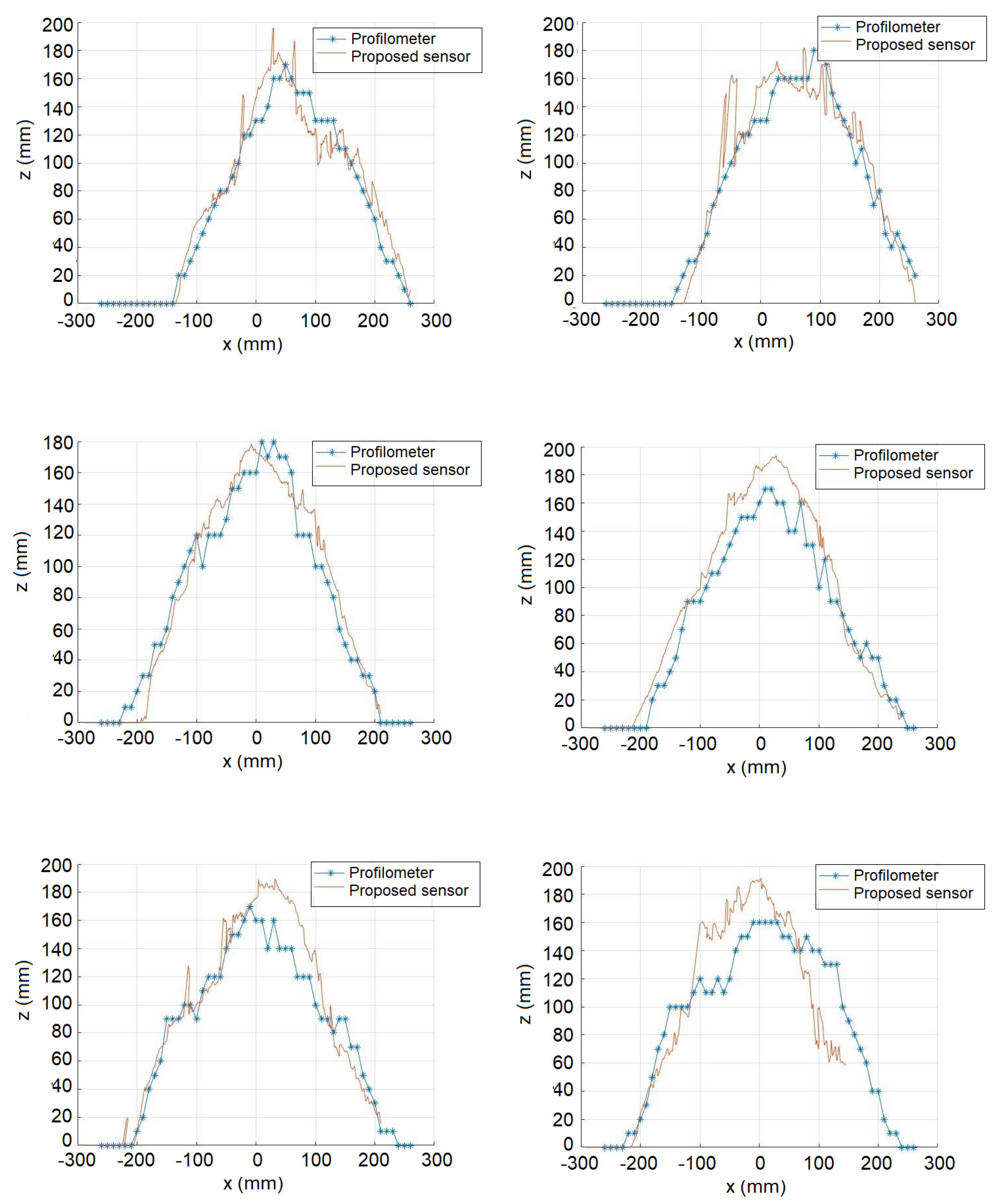
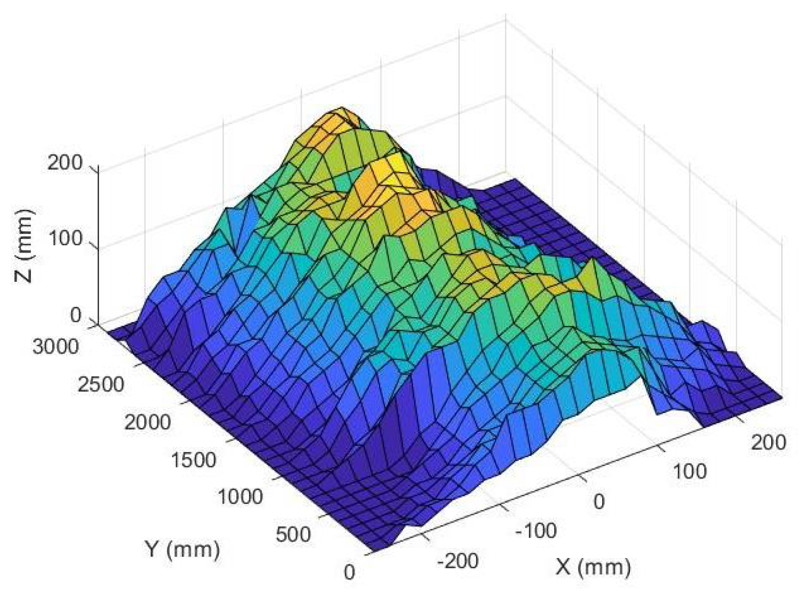
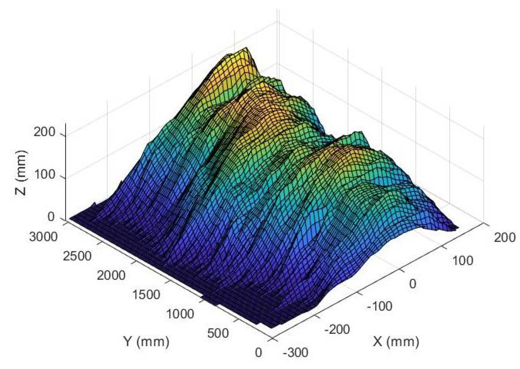
4.4. Triangulation

As the final stage of the proposed system, the triangulation stage shows the final shape of the bed at the point where the laser beam was projected. Figure 30 and Figure 31 show the results for various points sampled in the soil by superimposing the obtained data with the profilometer and the proposed system.

As the profilometer only produces point measurements, based on bars separated by a certain distance, the profile generated with its measurements is quite precarious. The system based on the proposed sensor, on the other hand, is based on a point cloud obtained by triangulating the laser projection points, providing great precision.

The root mean square error obtained by comparing the reconstruction result with the profilometer measurements is 28.86 mm.

With the data collected using the profilometer and the proposed system, it was possible to plot the 3D soil profiles. Figure 32 shows the reconstruction of the bed profile based on the profilometer reading.

Figure 33 shows the reconstruction of the windrow profile based on the reading of the proposed sensor.

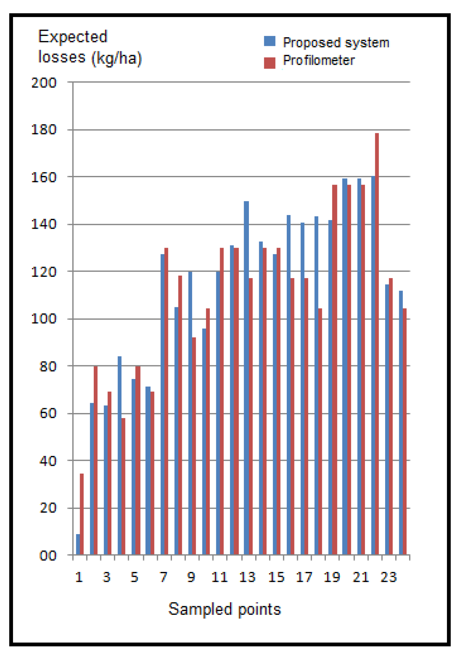
4.5. Estimated Losses

Based on the results obtained in [33], the points that correlate harvesting losses as a function of the height of the bed were drawn up, as shown in

Table 1. Estimated harvest losses according to windrow height.

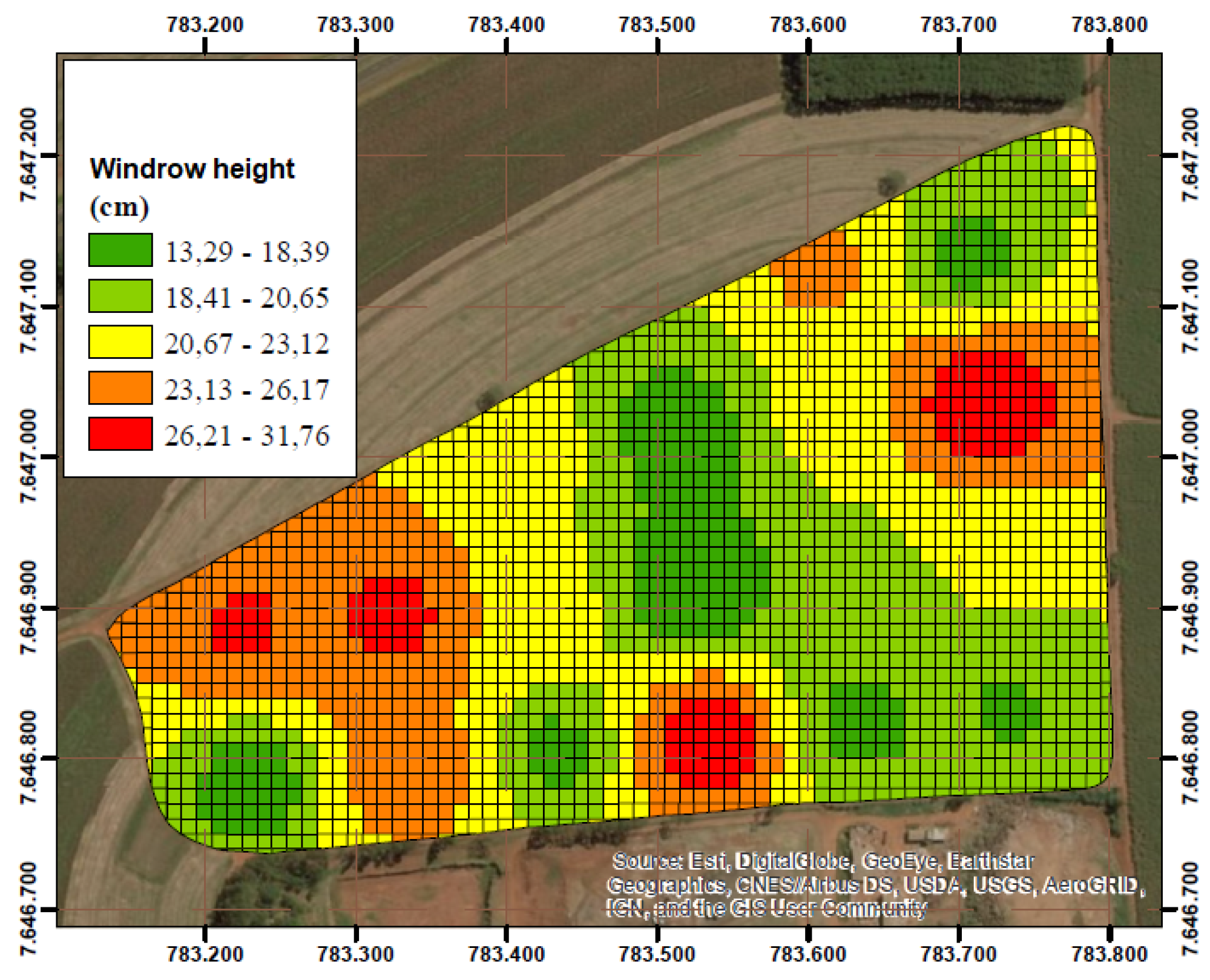
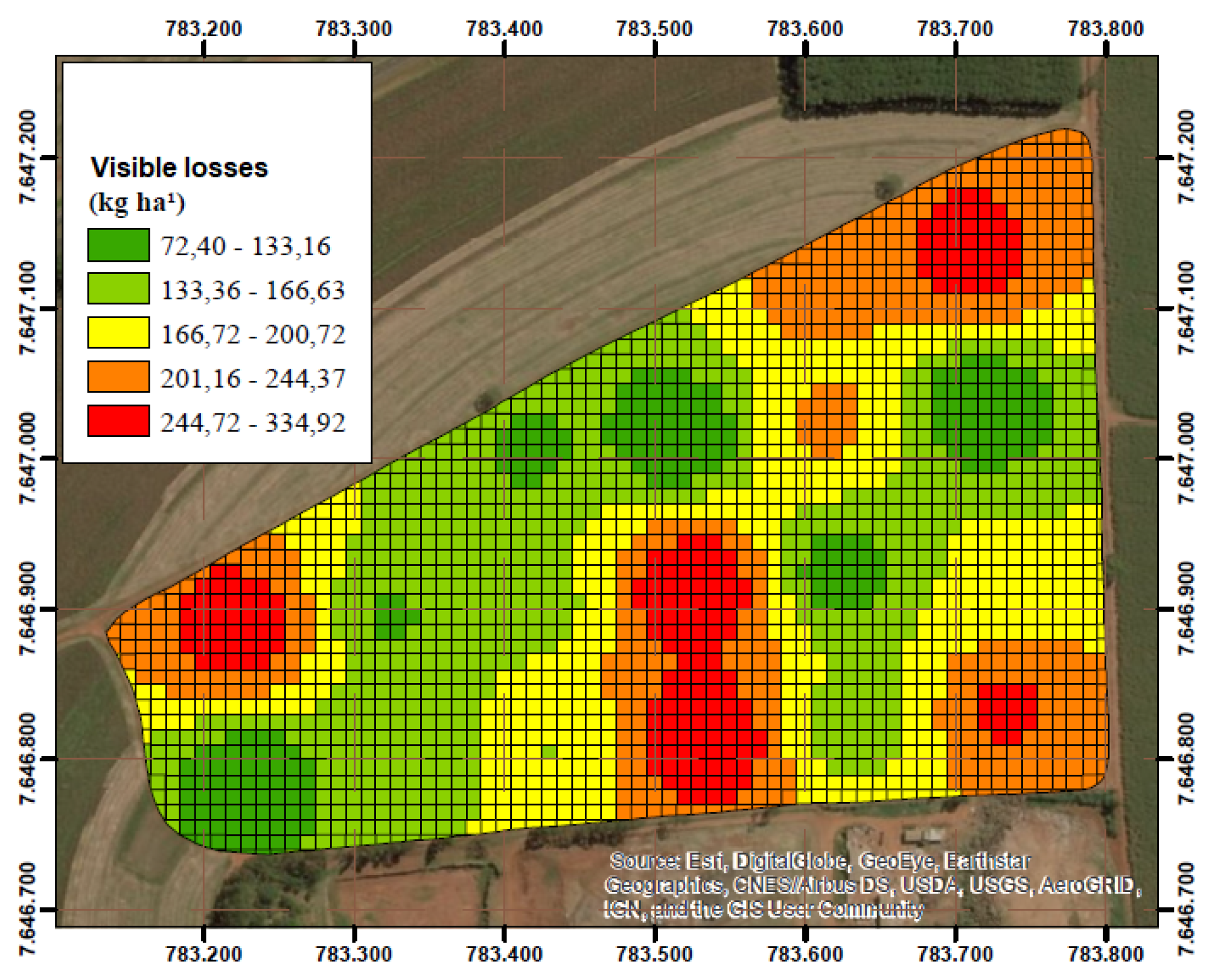
Windrow Height	Estimated Losses
13.29–18.39	72.40–133.16
18.41–20.65	133.36–166.63
20.67–23.12	166.72–200.72
23.13–26.17	201.16–244.37
26.21–31.76	244.72–334.92

.

The curve expressing the relationship between the height of the bed and the estimated losses in mechanized harvesting was drawn. This relationship is shown in Equation (25).

$$\begin{array}{c}\hfill y=0.1366x^2+8.10x-60.14\end{array}$$

(25)

For dynamic use, coupled with the digging/inversion system, the proposed method takes Equation (25) into account, i.e., for each sampled point, the profile of the bed, its maximum point and the expected losses for that point are considered. With the expected loss value, it is possible to dynamically alter the mechanism that does the grubbing, seeking to adjust the height of the formed bed to minimize losses. Figure 34 illustrates the concept.

By using the data from Equation (25) and the data obtained in the experimental analysis, it was possible to plot the expected losses for the obtained points using the maximum point of the profile obtained by triangulation and through the use of a profilometer for each sampled point. Figure 35 shows the correlation. Twenty-four sampling points were considered on the ground, spaced 10 cm along the length of the windrow. The proposed method provides a much more accurate analysis of the maximum point of the bed, resulting in a more detailed loss expectancy survey. These expected loss values act as a set point for the cutting-blade height control system of the digging–inverting mechanism and allow for closed-loop control of the mechanism. This control loop can be used to reduce digging losses and increase productivity per hectare.

5. Conclusions

In this paper, we present a system for estimating the windrow profile during mechanized peanut harvesting based on the incidence of an infrared laser beam on the ground under investigation. The process of acquiring images in pairs improves the task of segmenting the projection of the beam on the image, making the system less susceptible to interference from natural lighting. The proposed segmentation stage was implemented based on the specific characteristics of the application, which allowed for better precision. Additionally, the beam detection algorithm leverages the specific characteristics of the images to eliminate false positives and improve the performance of the reconstruction system. When comparing the results obtained with the proposed system to those obtained using a profilometer, it is evident that the proposed system is highly accurate, as it takes into account a cloud of points rather than just point measurements. The curve representing the windrow provides extensive information (maximum height point, width, shape, etc.), which can be used to dynamically adjust the digging/inversion system. Consequently, losses during this process can be minimized using the equation that correlates losses with the height of the bed.

Finally, mechatronic devices can be used to modify the reconstruction device’s d and $\theta$ parameters in real time in order to optimize the sensor’s coverage area and accuracy. The use of multiple beams at different wavelengths is a possible alternative for dealing with a greater variety of structures in the scene.

References

- Fasiolo, D.T.; Scalera, L.; Maset, E.; Gasparetto, A. Towards autonomous mapping in agriculture: A review of supportive technologies for ground robotics. Robot. Auton. Syst. 2023, 169, 104514. [Google Scholar] [CrossRef]
- Manish, R.; Lin, Y.-C.; Ravi, R.; Hasheminasab, S.M.; Zhou, T.; Habib, A. Development of a miniaturized mobile mapping system for in-row, under-canopy phenotyping. Remote Sens. 2021, 13, 276. [Google Scholar] [CrossRef]
- Baek, E.-T.; Im, D.-Y. ROS-based unmanned mobile robot platform for agriculture. Appl. Sci. 2022, 12, 4335. [Google Scholar] [CrossRef]
- Garrido, M.; Paraforos, D.S.; Reiser, D.; Arellano, M.V.; Griepentrog, H.W.; Valero, C. 3D maize plant reconstruction based on georeferenced overlapping LiDAR point clouds. Remote Sens. 2015, 7, 17077–17096. [Google Scholar] [CrossRef]
- Chebrolu, N.; Lottes, P.; Schaefer, A.; Winterhalter, W.; Burgard, W.; Stachniss, C. Agricultural robot dataset for plant classification, localization and mapping on sugar beet fields. Int. J. Robot. Res. 2017, 36, 1045–1052. [Google Scholar] [CrossRef]
- Cubero, S.; Marco-Noales, E.; Aleixos, N.; Barbé, S.; Blasco, J. Robhortic: A field robot to detect pests and diseases in horticultural crops by proximal sensing. Agriculture 2020, 10, 276. [Google Scholar] [CrossRef]
- Gasparino, M.V.; Higuti, V.A.; Velasquez, A.E.; Becker, M. Improved localization in a corn crop row using a rotated laser rangefinder for three-dimensional data acquisition. J. Braz. Soc. Mech. Sci. Eng. 2020, 42, 1–10. [Google Scholar] [CrossRef]
- Pire, T.; Mujica, M.; Civera, J.; Kofman, E. The Rosario dataset: Multisensor data for localization and mapping in agricultural environments. Int. J. Robot. Res. 2019, 38, 633–641. [Google Scholar] [CrossRef]
- Underwood, J.; Wendel, A.; Schofield, B.; McMurray, L.; Kimber, R. Efficient in-field plant phenomics for row-crops with an autonomous ground vehicle. J. Field Robot. 2017, 34, 1061–1083. [Google Scholar] [CrossRef]
- Kragh, M.F.; Christiansen, P.; Laursen, M.S.; Larsen, M.; Steen, K.A.; Green, O.; Karstoft, H.; Jø rgensen, R.N. Fieldsafe: Dataset for obstacle detection in agriculture. Sensors 2017, 17, 2579. [Google Scholar] [CrossRef]
- Krus, A.; Van Apeldoorn, D.; Valero, C.; Ramirez, J.J. Acquiring plant features with optical sensing devices in an organic strip-cropping system. Agronomy 2020, 10, 197. [Google Scholar] [CrossRef]
- Grimstad, L.; From, P.J. The Thorvald II agricultural robotic system. Robotics 2017, 6, 24. [Google Scholar] [CrossRef]
- Shafiekhani, A.; Kadam, S.; Fritschi, F.B.; DeSouza, G.N. Vinobot and vinoculer: Two robotic platforms for high-throughput field phenotyping. Sensors 2017, 17, 214. [Google Scholar] [CrossRef] [PubMed]
- de Silva, R.; Cielniak, G.; Gao, J. Towards agricultural autonomy: Crop row detection under varying field conditions using deep learning. arXiv 2021, arXiv:2109.08247. [Google Scholar]
- Brito Filho, A.L.P.; Carneiro, F.M.; Souza, J.B.C.; Almeida, S.L.H.; Lena, B.P.; Silva, R.P. Does the Soil Tillage Affect the Quality of the Peanut Picker? Agronomy 2023, 13, 1024. [Google Scholar] [CrossRef]
- Santos, E. Produtividade e Perdas em Função da Antecipação do Arranquio Mecanizado de Amendoim; Universidade Estadual Paulista: Jaboticabal, Brazil, 2011. [Google Scholar]
- Cavichioli, F.A.; Zerbato, C.; Bertonha, R.S.; da Silva, R.P.; Silva, V.F.A. Perdas quantitativas de amendoim nos períodos do dia em sistemas mecanizados de colheita. Científica 2014, 42, 211–215. [Google Scholar] [CrossRef]
- Zerbato, C.; Furlani, C.E.A.; Ormond, A.T.S.; Gírio, L.A.S.; Carneiro, F.M.; da Silva, R.P. Statistical process control applied to mechanized peanut sowing as a function of soil texture. PLoS ONE 2017, 12, e0180399. [Google Scholar] [CrossRef]
- Anco, D.J.; Thomas, J.S.; Jordan, D.L.; Shew, B.B.; Monfort, W.S.; Mehl, H.L.; Campbell, H.L. Peanut Yield Loss in the Presence of Defoliation Caused by Late or Early Leaf Spot. Plant Dis. 2020, 104, 1390–1399. [Google Scholar] [CrossRef]
- Shen, H.; Yang, H.; Gao, Q.; Gu, F.; Hu, Z.; Wu, F.; Chen, Y.; Cao, M. Experimental Research for Digging and Inverting of Upright Peanuts by Digger-Inverter. Agriculture 2023, 13, 847. [Google Scholar] [CrossRef]
- dos Santos, A.F.; Oliviera, L.P.; Oliveira, B.R.; Ormond, A.T.S.; da Silva, R.P. Can digger blades wear affect the quality of peanut digging? Rev. Eng. Agric. 2021, 29, 49–57. [Google Scholar] [CrossRef]
- Ortiz, B.V.; Balkcom, K.B.; Duzy, L.; van Santen, E.; Hartzog, D.L. Evaluation of agronomic and economic benefits of using RTK-GPS-based auto-steer guidance systems for peanut digging operations. Precis. Agric. 2013, 14, 357–375. [Google Scholar] [CrossRef]
- Yang, H.; Cao, M.; Wang, B.; Hu, Z.; Xu, H.; Wang, S.; Yu, Z. Design and Test of a Tangential-Axial Flow Picking Device for Peanut Combine Harvesting. Agriculture 2022, 12, 179. [Google Scholar] [CrossRef]
- Shi, L.; Wang, B.; Hu, Z.; Yang, H. Mechanism and Experiment of Full-Feeding Tangential-Flow Picking for Peanut Harvesting. Agriculture 2022, 12, 1448. [Google Scholar] [CrossRef]
- Azmoode-Mishamandani, A.; Abdollahpoor, S.; Navid, H.; Vahed, M.M. Performance evaluation of a peanut harvesting machine in Guilan province, Iran. Int. J. Biosci.—IJB 2014, 5, 94–101. [Google Scholar]
- Ferezin, E.; Voltarelli, M.A.; Silva, R.P.; Zerbato, C.; Cassia, M.T. Power take-off rotation and operation quality of peanut mechanized digging. Afr. J. Agric. Res. 2015, 10, 2486–2493. [Google Scholar] [CrossRef]
- Bunhola, T.M.; de Paula Borba, M.A.; de Oliveira, D.T.; Zerbato, C.; da Silva, R.P. Mapas temáticos para perdas no recolhimento em função da altura da leira. In Conference: 14º Encontro sobre a cultura do Amendoim; Anais: Jaboticabal, Brazil, 2021. [Google Scholar] [CrossRef]
- Lia, L.; Hea, F.; Fana, R.; Fanb, B.; Yan, X. 3D reconstruction based on hierarchical reinforcement learning with transferability. Integr. Comput.-Aided Eng. 2023, 30, 327–339. [Google Scholar] [CrossRef]
- Hu, X.; Xiong, N.; Yang, L.T.; Li, D. A surface reconstruction approach with a rotated camera. In Proceedings of the International Symposium on Computer Science and Its Applications, CSA 2008, Hobart, TAS, Australia, 13–15 October 2008; pp. 72–77. [Google Scholar]
- Li, D.; Zhang, H.; Song, Z.; Man, D.; Jones, M.W. An automatic laser scanning system for accurate 3D reconstruction of indoor scenes. In Proceedings of the 2017 IEEE International Conference on Information and Automation (ICIA), Macao, China, 18–20 July 2017; pp. 826–831. [Google Scholar]
- Shan, P.; Jiang, X.; Du, Y.; Ji, H.; Li, P.; Lyu, C.; Yang, W.; Liu, Y. A laser triangulation based on 3D scanner used for an autonomous interior finishing robot. In Proceedings of the 2017 IEEE International Conference on Robotics and Biomimetics, ROBIO 2017, Macau, China, 5–8 December 2017; pp. 1–6. [Google Scholar]
- Hadiyoso, S.; Musaharpa, G.T.; Wijayanto, I. Prototype implementation of dual laser 3D scanner system using cloud to cloud merging method. In Proceedings of the APWiMob 2017—IEEE Asia Pacific Conference on Wireless and Mobile, Bandung, Indonesia, 28–29 November 2017; pp. 36–40. [Google Scholar]
- Schlosser, J.F.; Herzog, D.; Rodrigues, H.E.; Souza, D.C. Tratores do Brasil. Cultiv. Máquinas 2023, XXII, 20–28. [Google Scholar]
- Simões, R. Controle Estatístico Aplicado ao Processo de Colheita Mecanizada de Sementes de Amendoim; Universidade Estadual Paulista: Jaboticabal, Brazil, 2009. [Google Scholar]
- Ferezin, E. Sistema Eletrohidráulico para Acionamento da Esteira vibratóRia do Invertedor de Amendoim; Universidade Estadual Paulista: Jaboticabal, Brazil, 2015. [Google Scholar]