Abstract
The implementation of poultry houses with enhanced control over environmental variables represents a solution to the growing demands for production and animal welfare. This study assessed the internal environment of dark-house poultry houses for broilers on a weekly basis throughout a production cycle. Data were collected over six weeks, from March to April 2016 involving 40,000 Cobb500TM broilers. A Hobo® datalogger continuously monitored the temperature (°C), relative humidity (%), dew point temperature (°C), and black globe temperature (°C) at 15 min intervals. The indices analyzed included the temperature and humidity index (THI), the black globe and humidity index (BGHI), and enthalpy (H). In the first week, both the THI and BGHI indicated favorable conditions for the birds, with the THI ranging from 72.4 to 80 and the BGHI from 77 to 81.6. Between the second and fifth weeks, the THI conditions varied between thermal comfort and discomfort, from 56.6 to 72. In the sixth week, all indices indicated discomfort, reflecting increased metabolism and population density. The dark-house system demonstrated a feed efficiency of 51%, an accumulated mortality rate of 1.97%, and a total production of 99,873 kg of meat. The study highlights the importance of continuously monitoring and adjusting environmental conditions to optimize production and enhance bird welfare.
1. Introduction
Factors such as investments in breeding facilities and the adoption of advanced technologies have been decisive in consolidating Brazil’s global leadership in broiler chicken exports [1]. Among the available structural typologies, the “dark house” stands out as an intensive production system, equipped with automated systems that control variables such as temperature, relative humidity, wind speed, and light intensity. The precise control of these variables creates an optimized environment, allowing the animals to achieve their maximum productive performance [2,3,4], as well as reducing carcass condemnation due to locomotor issues and mortality rates [5]. Additionally, the ability to control lighting regulates the broilers’ activity cycles, improving feed conversion and growth [6].
Although this system presents various benefits, there is a wide range of materials used for lateral closure, aimed at isolating the internal environment from external conditions, which may facilitate or hinder the performance of the animals [7,8]. Given the scarcity of information regarding specific environments based on the materials employed in climate-controlled poultry houses, it is important to evaluate the dark-house system by considering the type of management adopted, the conditions of the internal environment, and the characteristics of the regional climate.
Broiler production presents specific challenges, particularly in high-density environments and regions with hot climates. Proper management of heat stress is essential, as the broilers’ accelerated metabolism, combined with their limited ability to dissipate heat, makes them particularly vulnerable to overheating [9]. Heat stress directly impacts productive performance, reducing feed intake and feed conversion efficiency, while also increasing mortality risks [10].
Broiler chicken production involves a dynamic cycle, in which environmental variables are regularly adjusted to meet the animals’ needs at different growth stages. The technologies used in dark-house facilities create a stable and comfortable environment, primarily mitigating issues related to heat stress, which directly affects productivity [11].
Heat stress occurs when there is an imbalance between the internal heat production of the broilers and their ability to dissipate it into the environment [12]. This imbalance, caused by both high and low temperatures, affects the physiological parameters and performance of the broilers [13,14]. In cold-stress situations, broilers utilize dietary energy to generate heat rather than promote growth. Conversely, in heat-stress conditions, energy is directed towards losing heat, resulting in reduced feed intake and feed conversion efficiency [15]. Stressful situations can occur over short or prolonged periods, with each bird responding individually to the intensity and duration of these events, directly impacting their health, welfare, and productivity [12,16].
To reduce animals’ responses to heat stress, various strategies can be adopted, including environmental enrichment [17] and dietary supplementation [18]. The implementation of effective thermoregulatory solutions involves physical modification of the environment, breeding heat-tolerant animals, and improving nutritional management and feed composition [19].
In relation to the environment, variables such as temperature, relative humidity, and wind speed can be assessed using specific indices that allow for a non-invasive evaluation of the animals’ thermal comfort [20,21]. The temperature and humidity index (THI) combines air temperature and relative humidity to provide an integrated measure of thermal comfort [22]. The black globe temperature and humidity index (BGHI) includes thermal radiation, offering a more comprehensive assessment of the environment as perceived by the broilers [23]. Enthalpy, on the other hand, indicates the amount of thermal energy that must be removed to ensure adequate survival conditions within the facility [24].
The practical applications of these indices to broiler production allow for the monitoring of environmental conditions, aiding in the identification of thermal discomfort and optimization of management. These indices can guide adjustments in ventilation, heating, and cooling practices, ensuring that the birds are in a conducive environment for growth and welfare.
Selecting an appropriate index to evaluate and manage the microclimate in poultry houses requires a careful analysis of factors, such model of the facility, the technology used, and the regional climate. Implementing and maintaining optimal environmental conditions based on these indices can reduce heat stress, optimize feed conversion, and increase productivity, promoting more sustainable and economically viable production [25].
Given the impact of these technologies on environmental and production management, this study aims to analyze the effectiveness of automated environmental control systems in dark-house facilities by investigating the weekly thermal dynamics and environmental indices, namely THI, BGHI, and enthalpy, throughout the broilers’ growth phases. The research seeks to identify the need for system adjustments to ensure maximum productive performance and promote a sustainable and economically viable environment.
2. Materials and Methods
2.1. Characterization of the Site and the Installation
The research was approved by the Federal University of Lavras Ethics Committee on the Use of Animals, registered under protocol number 030/16. The research was conducted in a commercial poultry house in the state of Minas Gerais, Brazil (21°03′13″ south latitude and 44°05′24″ west longitude and an altitude of 1050 m), from March to April 2016. According to the Köppen classification, the climate is mild humid subtropical (Cwb), with average temperatures in the hottest and coldest months of 17 °C and 14.3 °C, respectively [26].
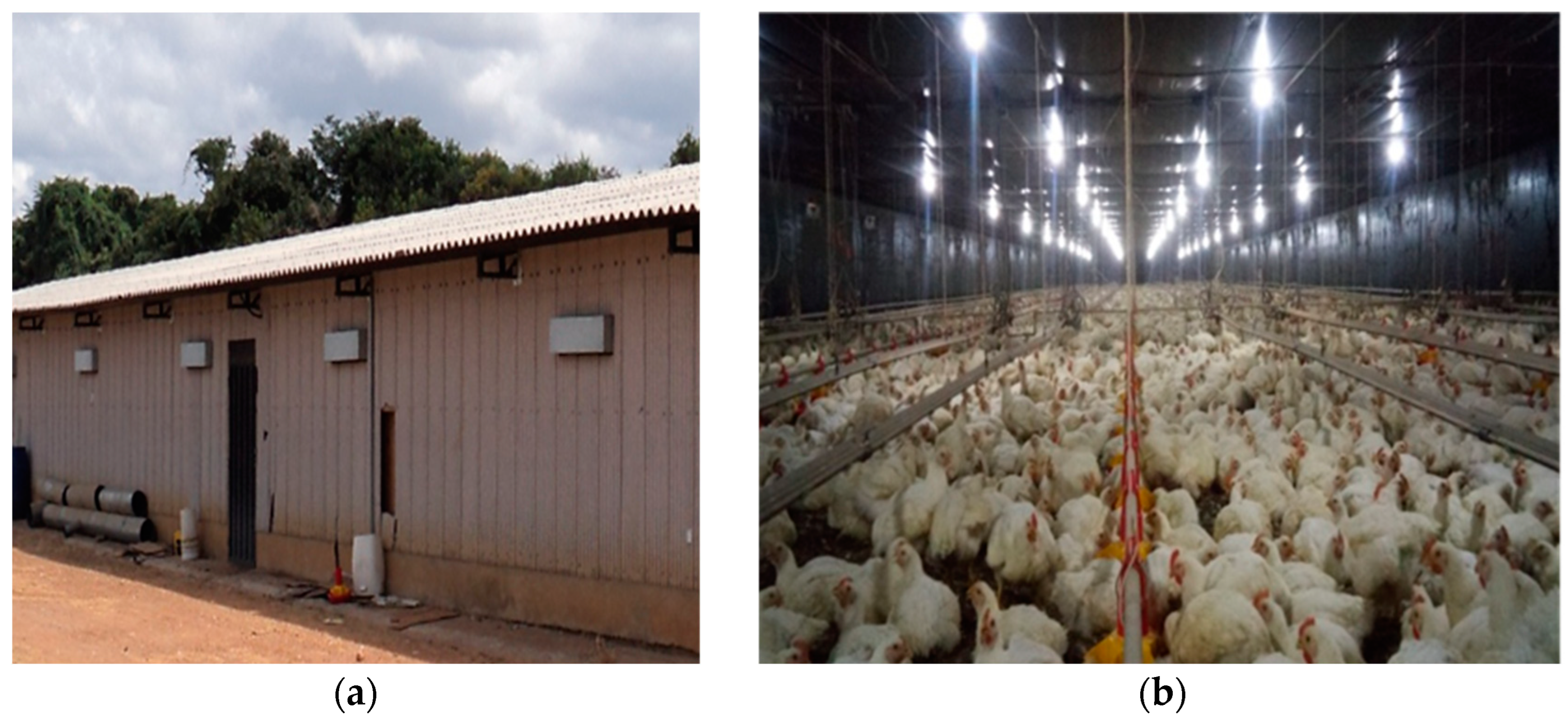
The aviary has dimensions of 150 m length, 18 m width, 2.80 m height, and an east–west orientation. The system has a lateral closure composed externally of fiber cement tiles and internally of plywood (painted black) supported on a 0.40 m high wall (Figure 1a). For illumination, the system has 89 LED lamps with a white color temperature of 7000 K and 8.6 W of power each (Figure 1b).
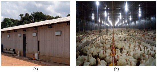
Figure 1.
External (a) and internal (b) view of the poultry house with sidewalls composed of fiber cement sheets and plywood.
The cooling of the poultry house is obtained by cellulose evaporative panels installed at one end of the shed and 16 1.0 HP exhaust fans opposite end. During the first two weeks of production, minimal ventilation is maintained with the evaporative panels operating continuously until the end of the cycle. To achieve minimal ventilation, 38 lateral inlets are used, which are made of galvanized steel sheets that open automatically due to pressure differences and the reduced, intermittent operation of the exhaust fans.
The roof of the sheds consists of six mm thick fiber cement roofing sheets with a 15% slope, with the ceiling lined with black tarpaulin. The heating system consists of two wood-fired stoves, model Vosser 4000 turbo, with dimensions of 2.70 m length, 1.20 m width, and 1.85 m height. Each stove is equipped with a 1/3 HP fan, two 2 HP motors, and an electronic panel for temperature control. The heated air is transferred to the interior of the poultry house through main ducts made of galvanized steel sheets, complemented by secondary ducts made of canvas. The poultry litter material used was sawdust, which was not reused.
The lighting program adopted throughout the experimental period was continuous (24 h of artificial light), using 25 lux from the 1st to the 25th day, followed by 5 lux until the end of the production cycle.
2.2. Operation of the Climate-Controlled Production System
The dark-house production system is characterized by a closed poultry house, with complete isolation between the internal and external environments. Generalizing, the system features an operations room equipped with a control panel that interacts with sensors installed in the production area and with predefined programs. This panel automatically activates the cellulose evaporative panels (with circulating water), heaters, inlets, exhaust fans, nebulizers, and lighting, ensuring the automation of environmental conditions.
The input values for the controller regarding the temperature and relative humidity of the production environment are determined by the producers according to the phase of development of the chickens. For those who are new to this system, these values are generally based on data from other properties. In some cases, the parameters are adjusted every seven days or at shorter intervals. In this experiment, the variations in reference values occur weekly.
The development cycle of broiler chickens is dynamic and can be divided into three main phases, namely the initial phase, from 1 to 14 days; the growth phase, from 15 to 35 days; and the finishing phase, from 36 days onwards. For each phase, there is an ideal range of temperature and relative humidity, which may vary according to the region and the genetics of the animal, ensuring adequate development. When the internal production environment deviates from these recommended ranges, the control panel automatically activates the equipment to adjust the internal conditions.
In the initial phase, the chicks require higher temperatures, necessitating a warmer environment. To meet this need, the controller activates the inlets, evaporative panels, and heaters, maintaining the environment under ideal conditions. As the chickens enter the growth phase, the heaters are turned off, and the controller gradually begins to operate the exhaust fans. In the final phase, if the evaporative panels and exhaust fans are insufficient to lower the internal temperature, the controller activates the nebulization system. The lighting control is achieved through the gradual reduction of the light intensity in the production environment, creating a space where the chickens remain calmer, which favors better conversion of the feed consumed. For this cycle, the producer opted not to gradually alter the lighting program, as described in Section 2.1.
Despite the automation of the system, it is essential to monitor and control all operations rigorously to avoid declines in productivity, which may result from inadequate regulation or excess humidity in the bedding. Given the level of technology involved and the potential fluctuations in the power supply, the use of energy generators becomes indispensable.
The direct effects of these operations are observed daily in the mortality counts and the visual characteristics of the development of the birds. This research employed independent sensors to monitor the environmental conditions provided by this control system.
2.3. Animals Housed and Measurement of Environmental Variables
Forty thousand mixed-sex broiler chickens of the Cobb500TM lineage, with an initial weight of 46.6 g and a final density of 39 kg/m2, were housed during a production cycle lasting 42 days.
The variables air temperature (t, °C), dew point temperature (dpt, °C), black globe temperature (bgt, °C), and relative air humidity (RH, %) were recorded over 42 days of age, using portable dataloggers from the Hobo® brand (Onset, Sigma Sensors, São José dos Campos, Brazil), model U12-013, with an accuracy of ±0.35 °C for temperature and ±2.5% for relative humidity. The dataloggers have two external channels, one of which is coupled to the external temperature sensor and inserted into a black globe, with a diameter of 15 cm painted with matte black paint. The sensors were distributed in nine points (Figure 2), with height adjusted according to the age of the poultry and programmed to collect and record data every 15 min for 24 h.

Figure 2.
Diagram of distribution of dataloggers inside the poultry house.
2.4. Spatialization of Environmental Comfort Indices
The collected variables were used to calculate the index temperature and humidity index (THI), black globe temperature index (BGHI), and the thermodynamic property, enthalpy (H).
In determining the THI, the equation proposed by Thom [22] was applied:
where
THI = t + 0.36 dpt + 41.5
t = air temperature (°C);
dpt = dew point temperature (°C).
The BGHI responsible for indirectly quantifying the effects of ventilation and radiation was calculated using the equation proposed by Buffington et al. [23]:
where
BGHI = bgt + 0.36 dpt + 41.5
bgt = black globe temperature (°C);
dpt = dew-point temperature (°C).
Enthalpy (H) is a physical property of thermodynamics and is also used as an indicator of comfort in a system. It provides the amount of thermal energy to be removed from the environment to provide thermal comfort for the animals. The enthalpy was calculated according to the equation proposed by Rodrigues et al. [24]:
where
H = enthalpy (kJ kg of dry air−1);
t = air temperature (°C);
RH = relative humidity (%);
BP = local barometric pressure (mmHg).
The recorded and calculated data were initially subjected to a descriptive analysis, defining parameters such as the mean, median, coefficient of variation, asymmetry, kurtosis, and standard deviation.
To identify the dispersion and spatial dependence of environmental variables and indices, geostatistical techniques were applied using the GS+® version 10 software. The semivariance was estimated by Equation (4), as described by Bachmaier and Backes [27]:
where
N(h) is the number of sampled pairs Z(Xi);
Z(Xi + h) are positions separated by a distance of h.
For the semivariance adjustment, the following models were applied: spherical, exponential, and Gaussian [28]. The parameters nugget effect (C0), contribution (C0 + C1), and amplitude (a) were obtained from the semivariance equation adjusted according to the behavior of the graphs.
The quality of adjustment was assessed by the degree of spatial dependence (DSD) according to the classification that considers values greater than 75% as weak spatial dependence; values between 25% and 75% as moderate spatial dependence; and values below 25% as strong spatial dependence [29]. The choice of model was also determined by the highest coefficient of determination (R2) and the lowest sum of squared residuals (SSR) [30,31]. After analyzing the spatial dependence, kriging interpolation was performed with the Surfer® 13 software to construct the maps.
2.5. Productive Responses
At the end of the production cycle, data on feed consumption and mortality were collected from the company to calculate production indicators.
The mortality rate refers to the percentage of broilers that die during the rearing cycle, from chick placement to slaughter, and is calculated according to Equation (5):
The mortality rate is a key indicator of the broilers’ health and welfare, as well as the efficiency of management, feeding, and biosecurity systems in a poultry house.
Feed efficiency in broiler production is a measure that reflects the impact of all actions taken throughout the production cycle on the broilers’ ability to convert feed into body weight gain, as shown in Equation (6):
Finally, the total meat production was calculated by multiplying the average live weight of the broilers by the total number of broilers at the end of the cycle. The efficiency of this production is influenced by factors such as broiler genetics, management, feeding, and rearing conditions throughout the production cycle.
3. Results and Discussion
The descriptive analysis of the recorded values aims to identify discrepant data, verify the normality of the frequency distribution, and analyze the data variation. To provide ideal conditions for animal development, environmental parameters must be homogeneously distributed in the production environment [32]. That said, Table 1 presents the descriptive analysis of the environmental variables investigated across all weeks.

Table 1.
Statistical indicators of the measures of position and dispersion for the variables analyzed throughout the production cycle, including temperature (°C), relative humidity (%), temperature and humidity indices (THI), black globe temperature and humidity index (BGHI), and enthalpy (H).
The coefficient of variation (CV) allows for the comparison of sample variability and the determination of experiment precision, serving as an indicator of the homogeneity of the collected data. According to Xue et al. [33], CV intervals of ≤10%, 10% < CV ≤ 100%, and CV > 100% indicate low, moderate, and high variability, respectively. Therefore, the experimentally collected data mostly present low variability, with weekly values below 10%. An exception occurred with ITU in the fourth and fifth weeks. However, these values are close to the lower limit of what is considered moderate variability.
The normal distribution of the data can be tested by comparing the mean and median values, in addition to the skewness and kurtosis. Based on these statistical indicators, a normal distribution with low skewness and leptokurtic distribution is observed, indicating a higher concentration of data near the mean. For geostatistical analysis, these features are desirable, as they indicate consistent spatial correlation and relationship within the dataset [34].
Random phenomena occurring in an environment can be analyzed by spatial variability, which quantifies the correlation between variables to deal with aggregated predictions and uncertainties [35]. This enables spatial analysis to examine patterns of data distribution with high spatial variability across various agricultural systems [36,37,38,39,40]. In other words, in a specific area, it is possible to measure the degree of spatial dependence between samples [41], although there is no rule limiting the minimum number of samples to be studied. Table 2 presents the parameters of semivariogram fittings for the evaluated variables and indices.

Table 2.
Models and estimated parameters of the semivariograms for temperature (°C), relative humidity (%), temperature and humidity indexes (THI), black globe temperature and humidity index (BGHI), and enthalpy (H) in the different weeks of rearing.
For the evaluated weeks, the Gaussian model demonstrated the best fit for most weeks, with a success rate of 63.4%, followed by the spherical (26.6%) and exponential (10%) models. These models are preferred due to their ability to provide an amplitude value corresponding to the maximum distance of spatial dependence [42,43]. The Gaussian model, in particular, is known for its efficiency in predicting continuous phenomena, providing an unbiased estimate in regions with autocorrelated data, making it suitable for estimating spatial variability in various environmental factors [44,45].
The relevant piece of information extracted from the semivariogram is the practical range (A), which indicates the distance within which the variable is spatially correlated between the assessed points [39]. For the variables t and THI, regardless of the week evaluated, the range obtained was greater than the distance between the collection points (37.5 m), indicating that, in isolated environments, it may be possible to reduce the number of samples. Ranges smaller than the distance between the collection points were identified in specific situations, with RH in the fifth week (19.3 m), BGHI in the second week (27.62 m), and H in the first and second weeks (28.07 m and 17.79 m, respectively). These distances allow the overlap of the range radii around the sampled points.
The nugget effect (C0) is a parameter of the semivariogram that denotes an unexplained variability [46]. Thus, the smaller C0 is, the greater the spatial dependence and, consequently, the better the estimate by kriging [7,47]. According to the classification by Cambardella et al. [29], the DSD was characterized as strong for most weeks in all variables (Table 2), suggesting good accuracy in the estimation of the behavior of indices and environmental variables using spatial distribution maps.
The spatial variability analysis also demonstrated strong results, showing a high degree of spatial dependence (DSD) in the evaluation of environmental factors in poultry farms across various regions of Brazil [30,39,47,48,49].
In certain situations, especially during the first week, low R2 values were observed for the variables t, RH, and BGHI, as well as for the variable H in the second, third, and fourth weeks. This result does not indicate an absence of correlation between the observed and model-predicted values, since the data may have a curvilinear, rather than a linear, relationship [50]. Furthermore, a low R2 means that other factors, such as randomness, are affecting the variability of the data. Therefore, when evaluating a geostatistical model, other factors should be considered, such as the lowest SSR and C0, and the best DSD.
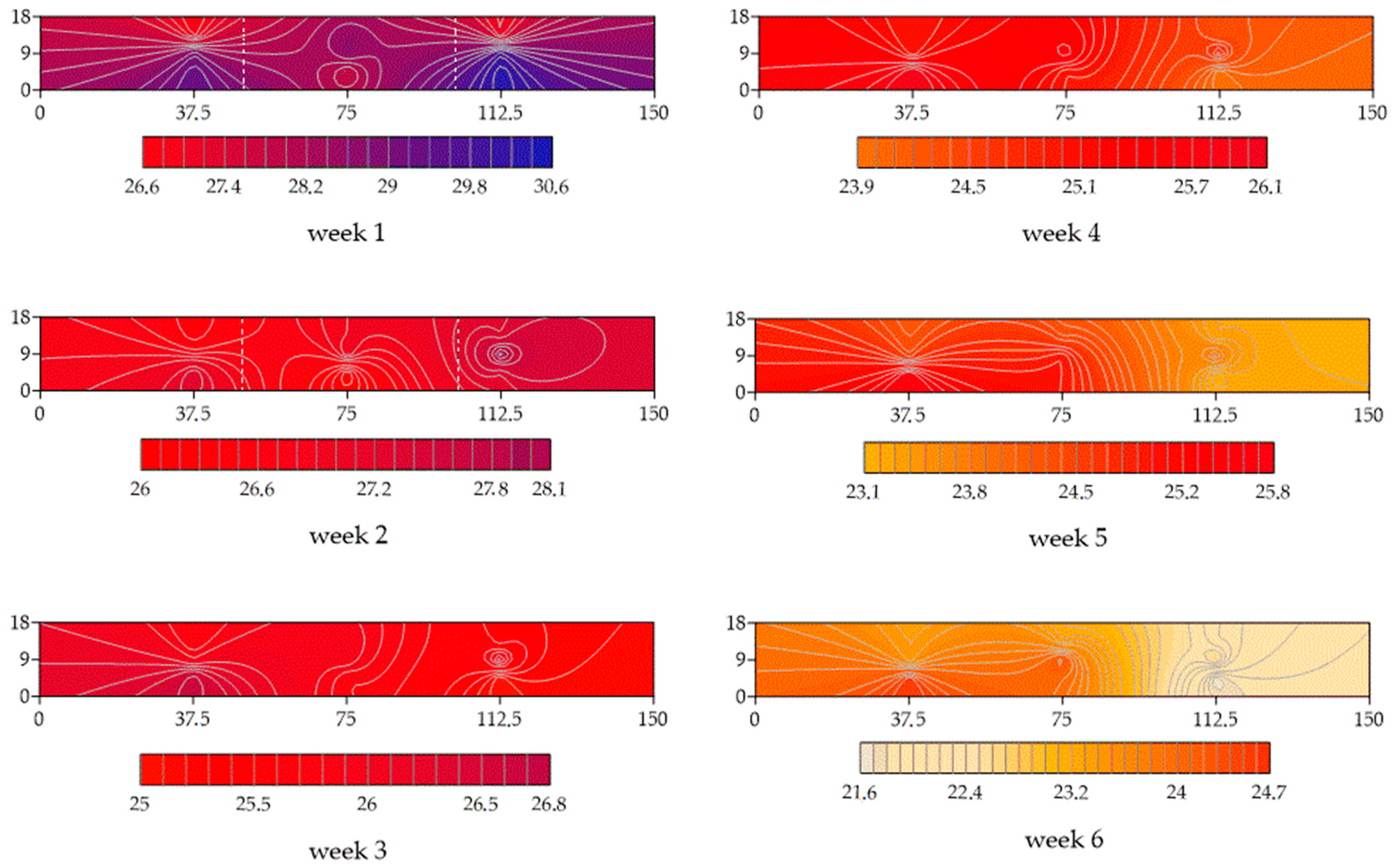
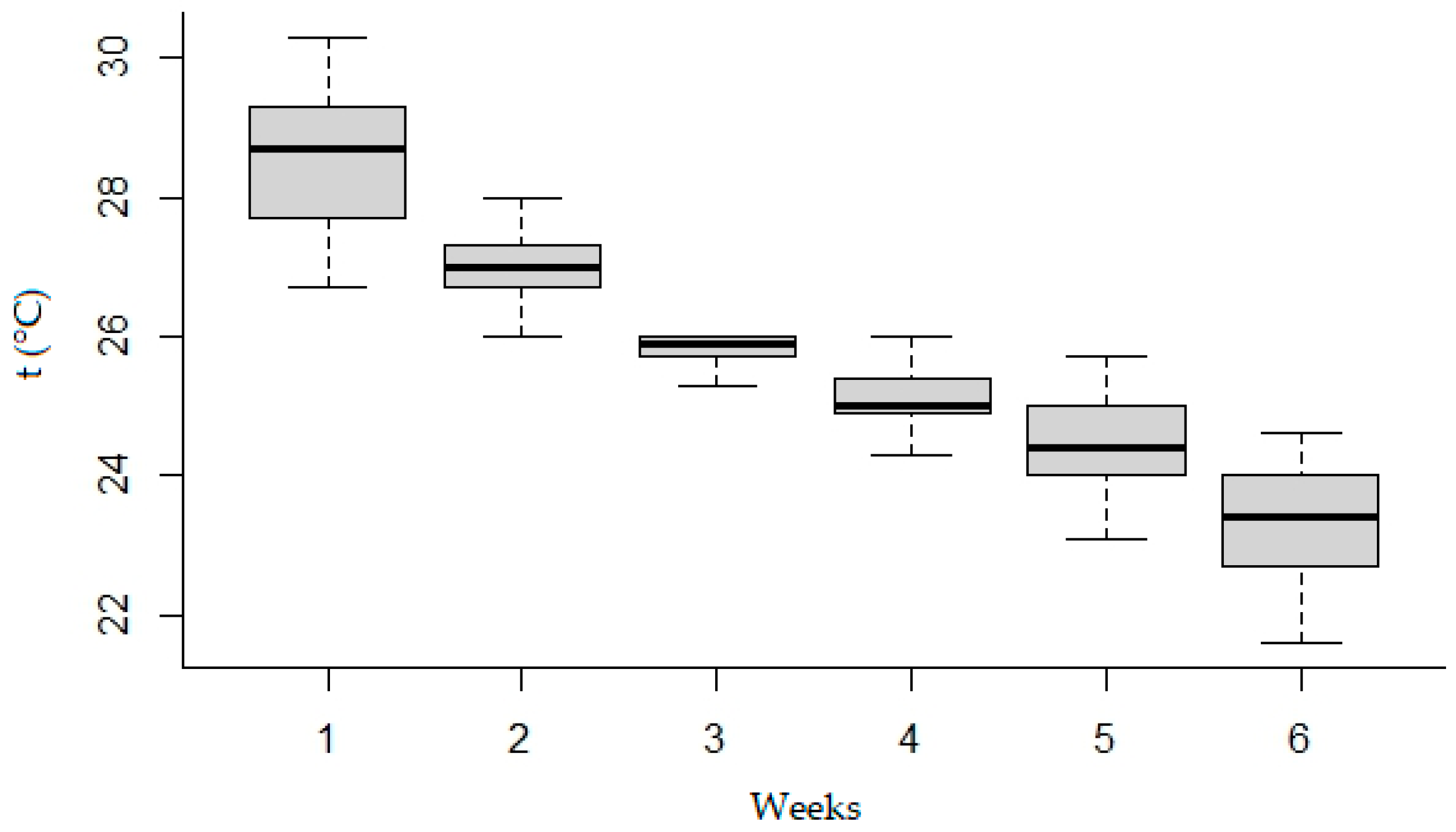
Kriging maps allow for the visualization of the spatial distribution of the evaluated variables. Figure 3 shows the distribution of temperature (t, °C) within the poultry house on a weekly basis, while Figure 4 illustrates the weekly variation in temperature.

Figure 3.
Kriging maps for the temperature (t, °C) throughout the shed in the six weeks of rearing.
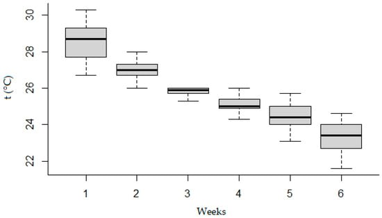
Figure 4.
Weekly distribution of temperature (°C) inside the poultry house throughout the production cycle.
The first and second weeks of age comprise the heating phase, during which only the central area of the shed (indicated by a dashed line) is used to house the animals, being separated by tarps fixed from the ceiling to the floor (east facing). According to Medeiros et al. [51], the temperature should vary between 32 and 34 °C during the first week of life and between 28 and 32 °C during the second week. Figure 3 indicates that, in the chick housing area (weeks 1 and 2), despite little variation, the temperatures did not reach levels considered comfortable.
The ineffective management in the early weeks, evidenced by the low heating of the environment, can be attributed to the low external temperatures that occur in the region during this time of year. Additionally, operational errors in the amount of biomass added to the furnaces, as reported by Ferraz et al. [52], also contribute to this problem.
Exposure to thermal discomfort early in life can impair the performance of broilers, as their thermoregulatory system is not fully developed, leading to productivity losses throughout the production cycle [53]. From the 15th day of production, the chickens occupied the entire area of the shed, and the temperature varied from 26.7 °C to 24.6 °C in the region influenced by the exhaust fans (west face). This behavior aligns with the air-cooling flow direction and does not affect the animals’ functional capacity, as temperatures between 21 °C and 28 °C are within the thermoneutral zone [54]. Adequate monitoring of poultry housing is essential to minimize situations that lead to thermal stress, as temperatures above 20 °C result in a 6% increase in water consumption and a 1.23% reduction in feed consumption for each additional degree [55].
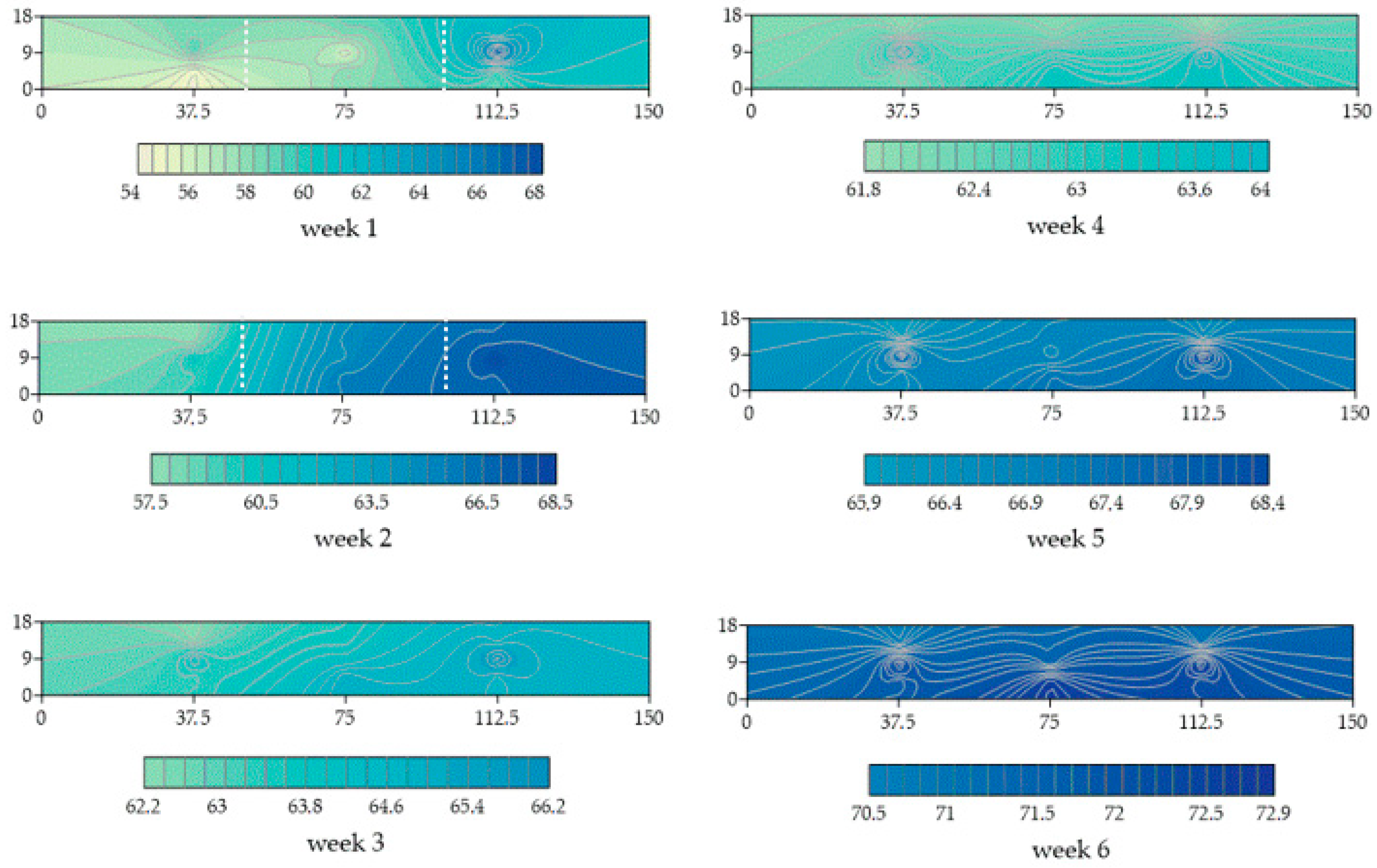
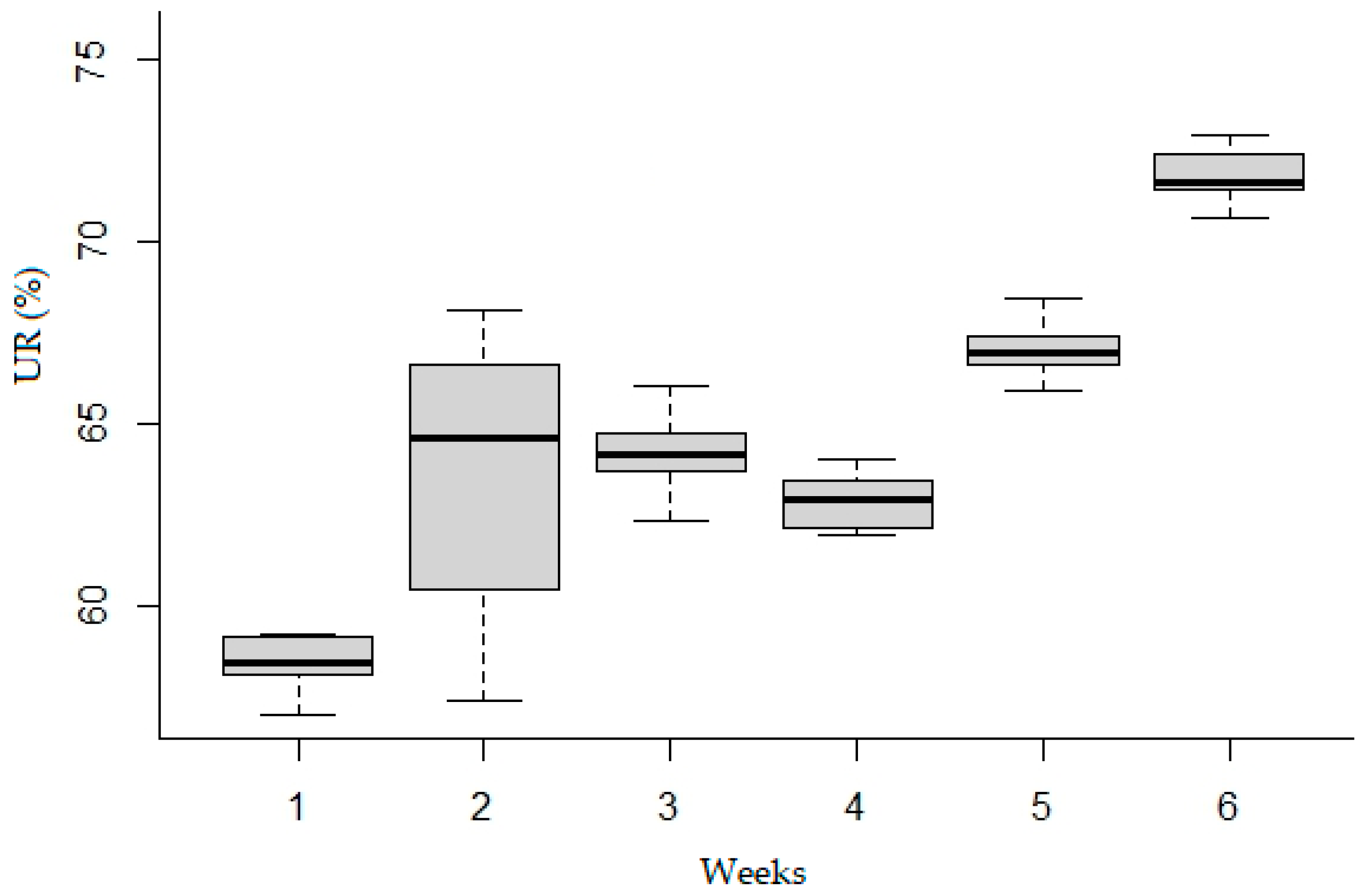
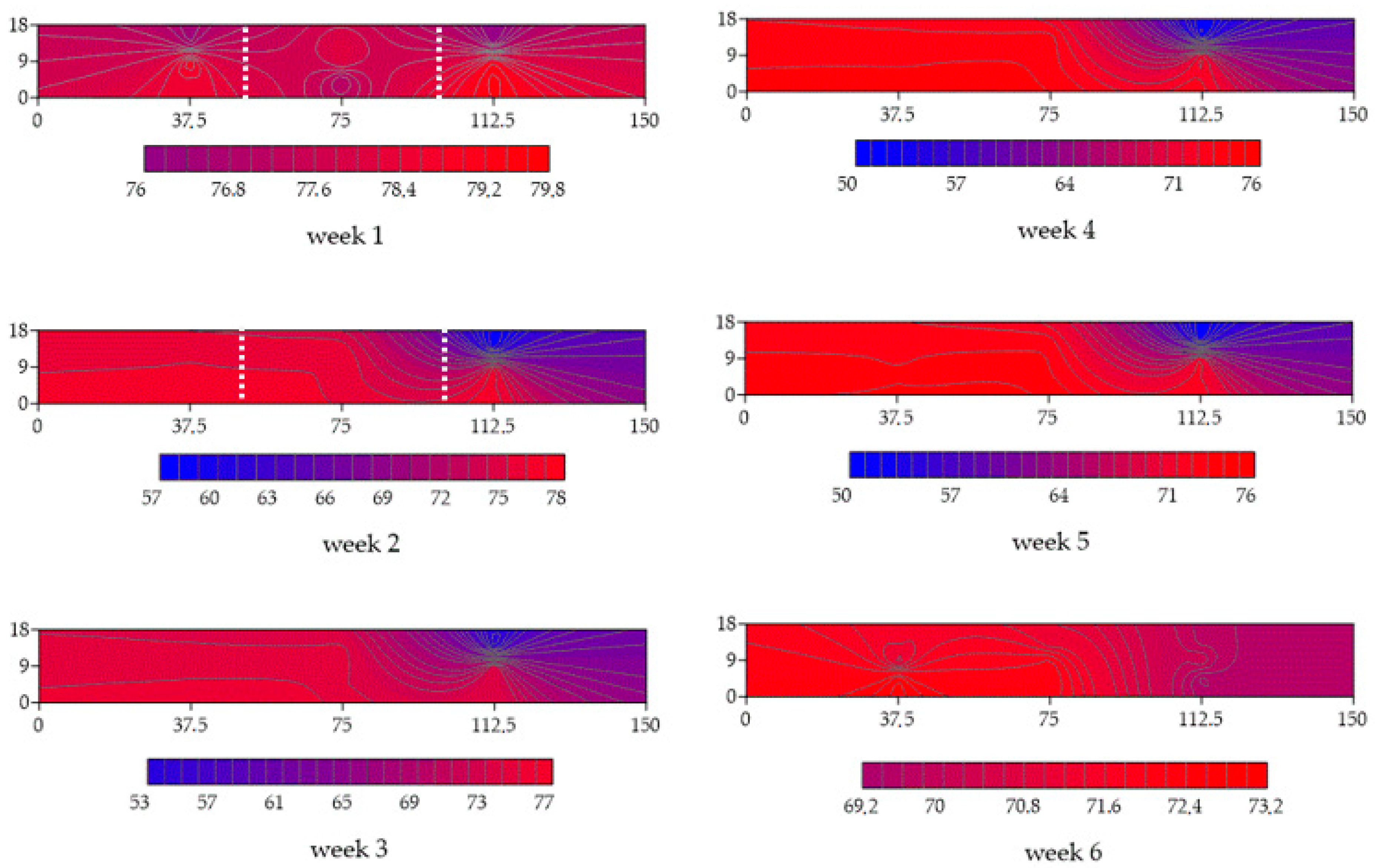
Heat dissipation by the animal is significantly influenced by relative humidity. Under high humidity, evaporative heat loss decreases [56]. Relative humidity (Figure 5 and Figure 6) increased from the first to the last week of production, ranging from 54.5% to 72.7%.
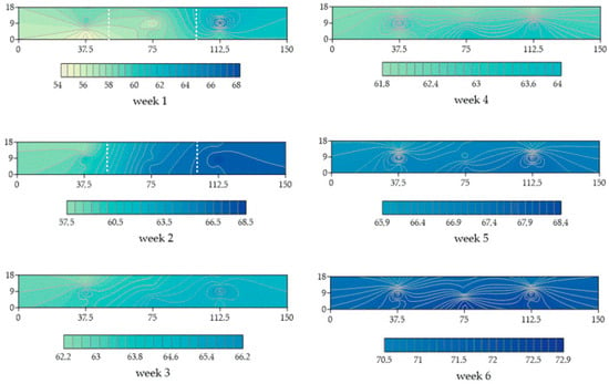
Figure 5.
Kriging maps for the relative air humidity (RH, %) throughout the shed in the six weeks of rearing.
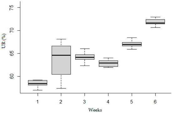
Figure 6.
Weekly distribution of relative humidity (%) inside the poultry house throughout the production cycle.
An exceptional condition occurred in the second week, where the evaporative panel region was still insulated, creating a dense area with humidity levels between 63% and 68%.
Despite the heterogeneity observed in all weeks, the RH values were within the range considered comfortable for broilers, varying from 50% to 80% [51,57]. The best performance of the animals can result from being kept in an environment with 80% RH [58] or in environments maintained close to 60% RH [59]. This difference is due to regional location and seasonal temperature variations. Therefore, temperature and RH are interdependent variables for characterizing the rearing environment and can be associated with environmental thermal indices, enabling analyses for the implementation of preventive and corrective operations in the environment.
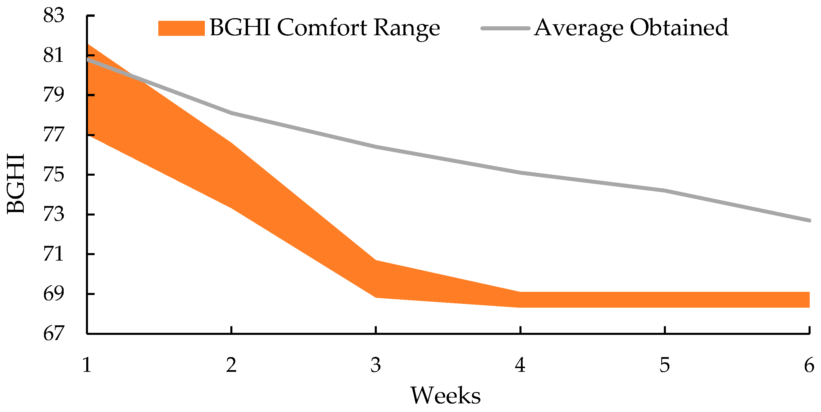
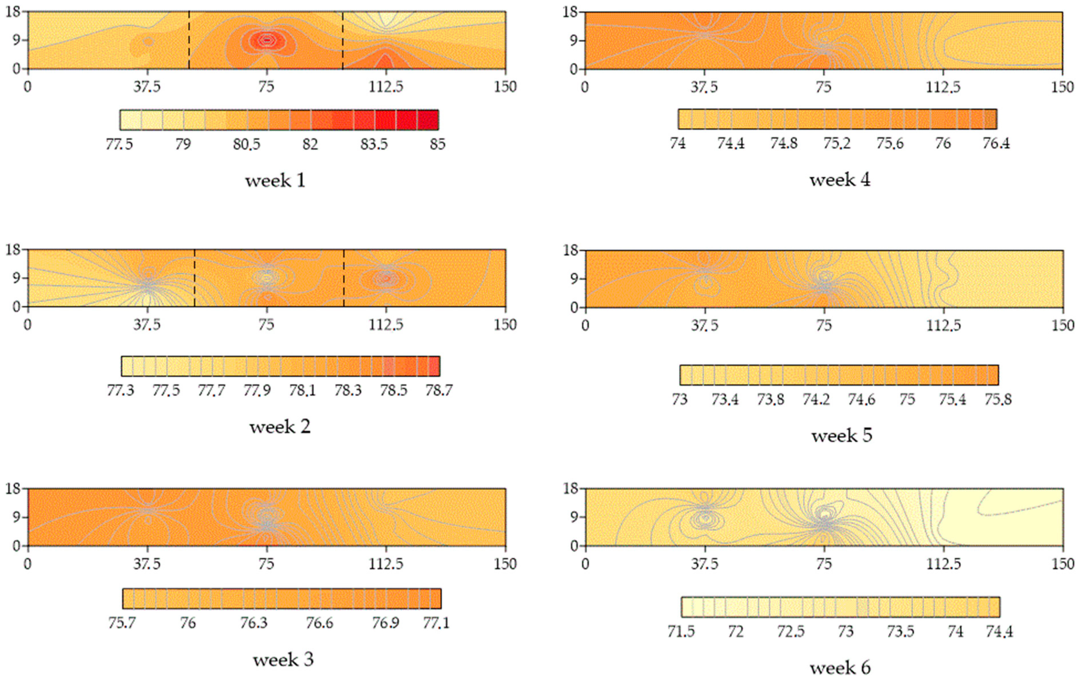
Thus, Figure 7 indicates the comfort range of THI with the weekly average obtained, and Figure 8 complements the information with the spatial distribution for the six weeks of rearing.
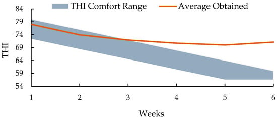
Figure 7.
Comfort range of THI with the average obtained. Adapted from de Silva et al. [60], Medeiros et al. [51], and Furtado et al. [61].

Figure 8.
Kriging maps for the temperature and humidity index (THI) throughout the shed in the six weeks of rearing.
Figure 7 reveals that, according to the THI index, the poultry house maintained thermal comfort conditions during the first three weeks, despite the temperatures being below the recommended level for the heating phase. The lowest THI values are found in the area influenced by the evaporative panels (Figure 8). According to Ferraz et al. [62], when areas with suboptimal thermal conditions are identified, it is important to assess the frequency with which the broilers were exposed to these adverse situations. In line with this, Figure 9 illustrates the frequency of THI occurrences over the six weeks of rearing, obtained through Kriging interpolation and based on the comfort limits.
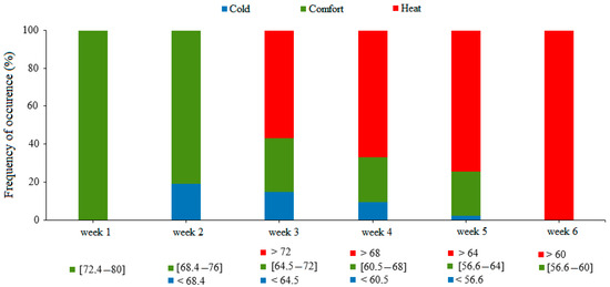
Figure 9.
Frequency of occurrence (%) of temperature and humidity index (THI) inside the shed during the rearing cycle.
Figure 9 reveals good consistency in environmental variables during the first and sixth weeks, corresponding to zones of total thermal comfort and thermal discomfort, respectively. Although the second week showed signs of stress due to low temperatures (Figure 9), the poultry-housing area remained in comfortable conditions (Figure 7). In weeks 3, 4, and 5, only 25% of the area was classified as comfortable, with occurrences of both cold and heat discomfort. To ensure productive uniformity in the flock, it is essential to maintain consistency in the thermal conditions of the environment [62].
Uncontrolled temperatures, along with other environmental factors, can cause metabolic disorders in broilers, such as ascites, leading to inactivity, lethargy, respiratory difficulties, and reduced growth [54]. However, a well-optimized dark-house poultry system is effective in mitigating these effects, as it allows for a reduction in the hours of light provided to the animals.
For broiler chickens, the use of the BGHI is a viable approach, as this index integrates radiation, temperature, relative humidity, and indirectly, wind speed, consolidating these climatic factors into a single value. Figure 10 illustrates the recommended range for the BGHI, and the average obtained in this study. Meanwhile, Figure 11 complements this by showing the distribution of the index within the poultry house.

Figure 10.
Comfort range for BGHI with the average obtained. Adapted from de Silva et al. [60], Medeiros et al. [51], and Furtado et al. [61].
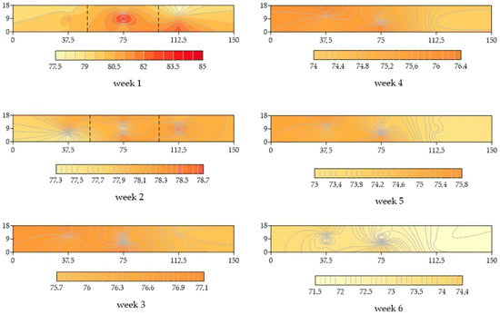
Figure 11.
Kriging maps for the black globe humidity index (BGHI) throughout the shed in the six weeks of rearing.
Similar to the THI, the BGHI indicated that the poultry house was in thermal comfort during the first week. However, in the following weeks, the average recorded was outside the comfort range. Figure 11 shows that this thermal discomfort occurs from the central region to the area near the exhaust fans. This issue may be related to the absence of “light traps” on the exhaust fans, resulting in increased external light entering the poultry house.
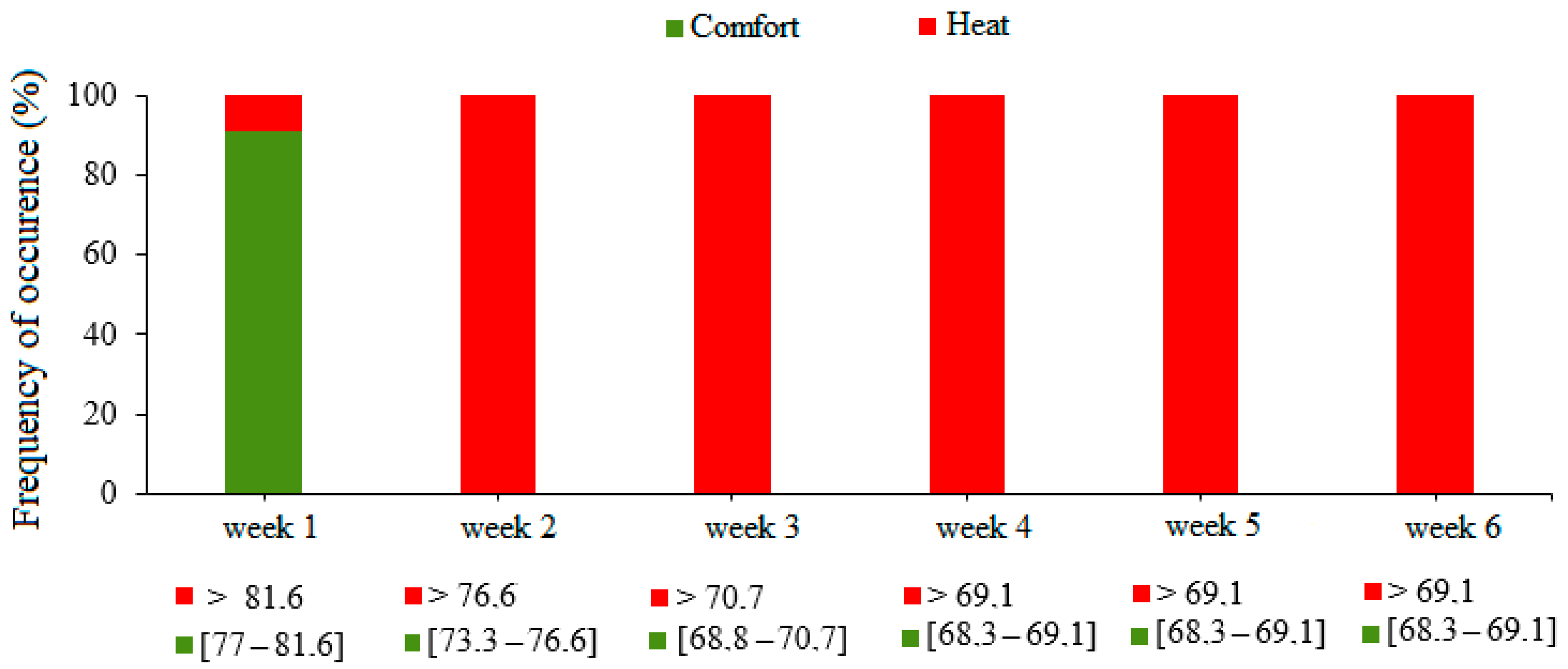
Upon analyzing the frequency (Figure 12), it is observed that, from weeks 2 to 6, the situation classified by the BGHI indicates thermal discomfort due to heat.
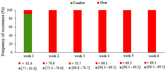
Figure 12.
Frequency of occurrence (%) of the black globe humidity index (BGHI) inside the shed during the rearing cycle.
Based on the frequency distributions, it was observed that, in the first week, 91% of the barn area met the recommended conditions for rearing. However, 9% of the area experienced thermal conditions in the discomfort zone due to high temperatures. This result may be influenced by the furnaces operating during the first week. For all subsequent weeks, the condition observed was that 100% of the environments exhibited thermal discomfort due to heat. The BGHI may not be effective when applied to isolated environments, such as the dark-house aviary.
For improved monitoring during the production cycle, alternatives based on variables that affect broiler performance are being developed, enabling producers to make swift and precise decisions about the environment, particularly regarding equipment adjustments [63,64].
Closed production systems, such as dark-house setups, which include exhaust fans, evaporative panels, light control, and a control room, are more effective in maintaining the environment and reducing the negative effects of thermal stress [65].
Like other indices, enthalpy has a range of recommended values that varies according to each week of the broilers’ development. The recommended range for H and the average obtained are indicated in Figure 13. In addition, the spatial distribution of this variable is visualized in Figure 14.
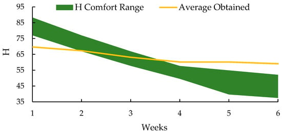
Figure 13.
Comfort range for H (kJ kg of dry air−1) with the average obtained. Adapted from Barbosa Filho et al. [66].
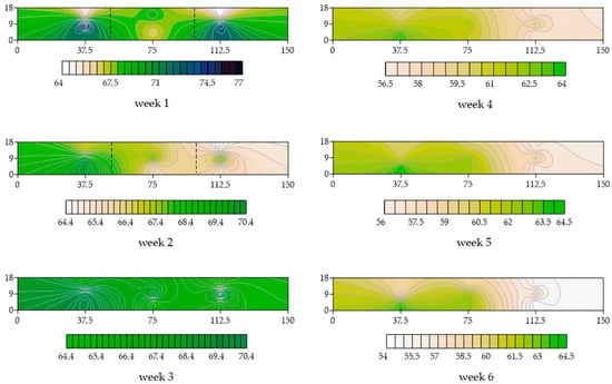
Figure 14.
Kriging maps for H (kJ kg of dry air−1) throughout the shed in the six weeks of rearing.
Thermal comfort environments indicated by enthalpy were observed in the second and third weeks of production, with a variation between the maximum and minimum values of six units (Figure 13 and Figure 14). The first week of production showed the greatest range of recorded values, with 12 units, and an environment below the comfort range (Figure 13). The spatial distribution in the fourth, fifth, and sixth weeks displayed similar behavior, with high H values recorded in the area near the exhausts (Figure 14). According to Moghadam et al. [67], the enthalpy index (H) is not able to assess well-being throughout the entire facility, as the heat produced by broiler chickens causes greater thermal discomfort in the central areas and near the exhausts compared to the regions close to the air inlets.
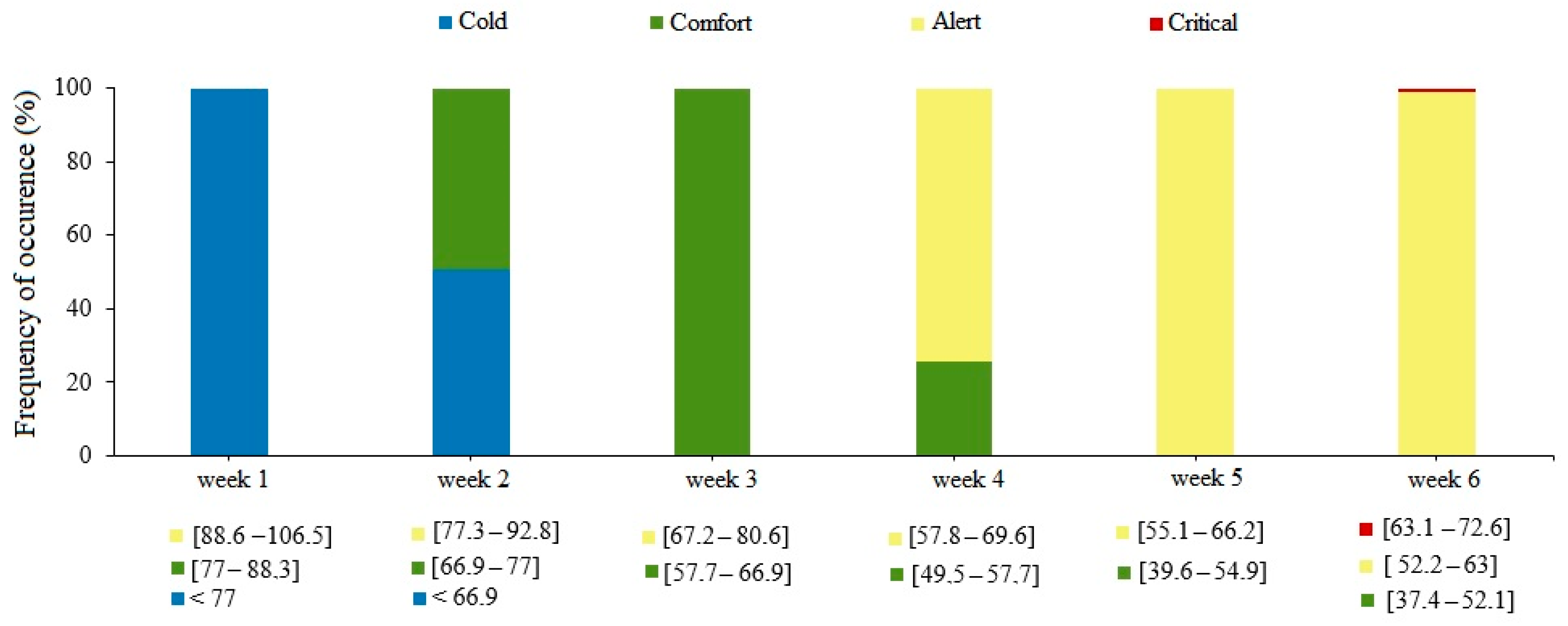
The performance of H inside the shed, according to its comfort classification, can be better seen in Figure 15.
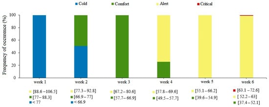
Figure 15.
Frequency of occurrence (%) of enthalpy (H) inside the shed during the rearing cycle.
Enthalpy, which reflects the amount of heat within the facility, revealed that the first week experienced a cold environment, reinforcing the occurrence of low temperatures during this period.
From the fourth week onwards, the enthalpy (H) recorded a higher frequency of alert conditions. Values of H in this situation require more stringent control of environmental variables, especially in the sixth week of production, which is critical and presents the highest productive losses [68]. Maintaining an adequate thermal environment in the final week of broiler production is challenging due to the increased metabolism, high population density, greater heat sensitivity, and climatic conditions.
In severe heat conditions, the significant increase in water consumption by broilers results in liquid feces and increased bedding moisture, reducing its absorption capacity and raising ammonia concentrations in the air to dangerous levels, which can lead to polypnea and even death if these conditions persist [51].
The results for H may be more satisfactory when the regional climatic conditions are considered, allowing for more precise adjustments to the internal equipment for each phase of the broilers’ development and for different seasons [25].
The construction features of poultry houses influence the internal microclimate. Therefore, assessing different management systems and identifying the most impactful variables are essential for defining a productive environment [30,69,70].
In turn, insufficient management during the production cycle results in inadequate and stressful thermal conditions in the poultry environment, which is a key factor in productive and economic losses in broiler production.
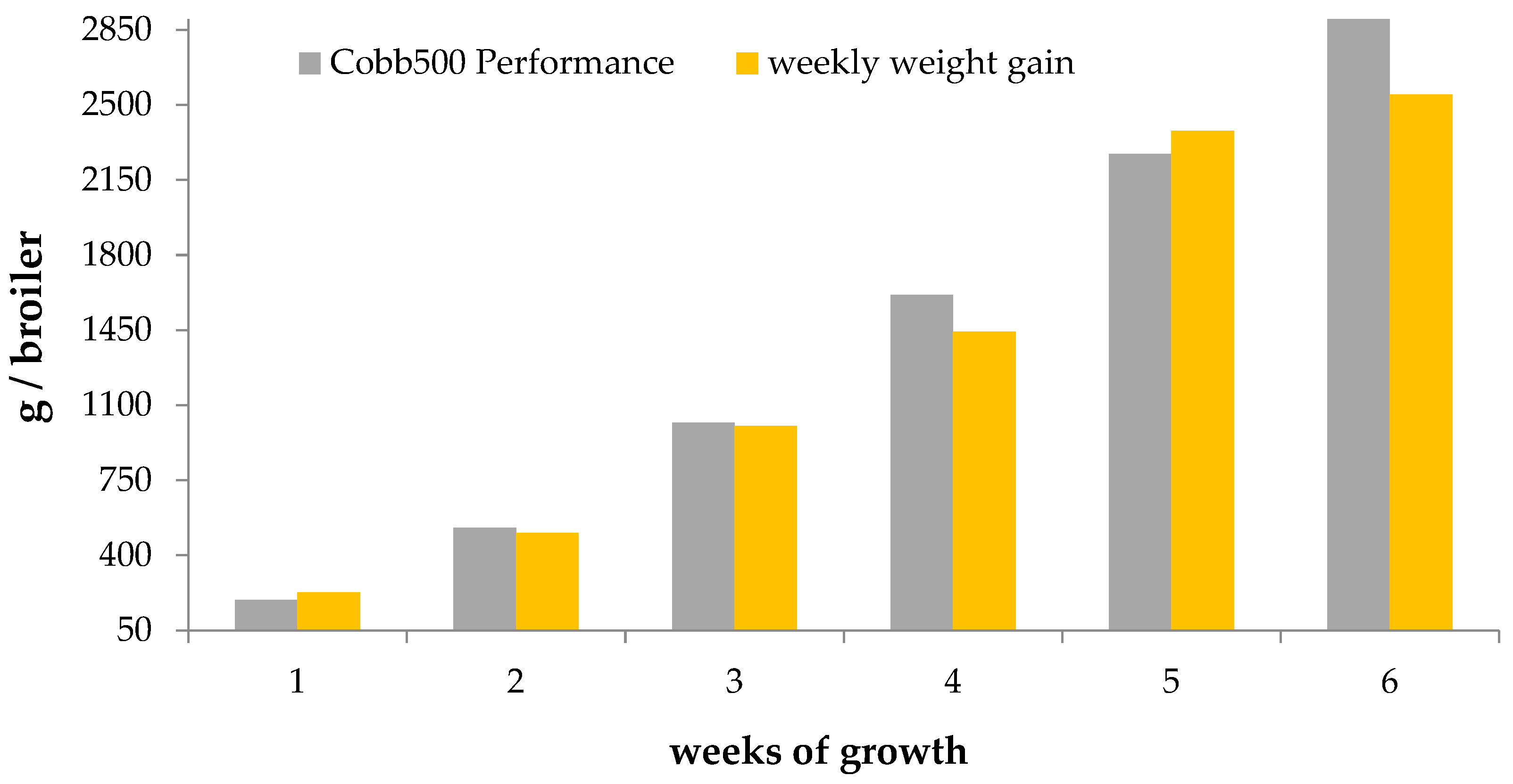
In terms of production, the dark-house system resulted in a production cycle with a feed efficiency of 51%, a low cumulative mortality rate of 1.97%, and a total meat production of 99,873 kg. The installation microclimate affects chickens of different genetic strains differently, influencing their development and feed consumption rate [21]. The weekly performance achieved for the Cobb500TM strain is indicated in Figure 16.
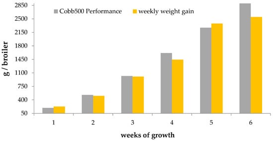
Figure 16.
Weekly weight gain in relation to the performance capability of the Cobb500TM lineage [71].
Weight gains exceeding the performance target for the lineage were observed in the first and fifth weeks of production. In the first week, despite temperatures not meeting the recommended levels in the literature, maintaining an environment with low thermal variability contributed to the broiler’s good development. Additionally, the dark-house system proved to be effective by balancing the external variables with the internal conditions during the first week.
The broilers achieved feed efficiency rates close to the target, with 95.5% in the second week and 98.5% in the third week. Conversely, weeks 4 and 6 displayed performance below the lineage target, with efficiency rates of 89.3% and 83.3%, respectively. These unfavorable conditions in the production environment resulted in a minimum loss of 24,590.46 kg of meat.
Weight gain, feed consumption, and feed conversion throughout the production cycle are also linked to feed formulation, making it important to adjust the size of maize particles for each stage of the chicken’s development [72]. A total of 192.75 tons of feed were provided, with formulations adjusted according to the age of the chickens, including starter for weeks 1 and 2; grower 1 for weeks 3 and 4; grower 2 for week 5; and finisher for week 6. At the end of the batch, the feed conversion ratio recorded was 1.97, with an average feed consumption of 4.92 kg per broiler, and each one reached an average weight of 2500.4 g.
The production cycle of broiler chickens is dynamic, with varying thermal requirements according to age. To optimize production and promote the health and welfare of the broiler, it is important to implement measures that ensure an adequate thermal environment, as discomfort conditions impair feed efficiency, increase mortality, and compromise final productivity.
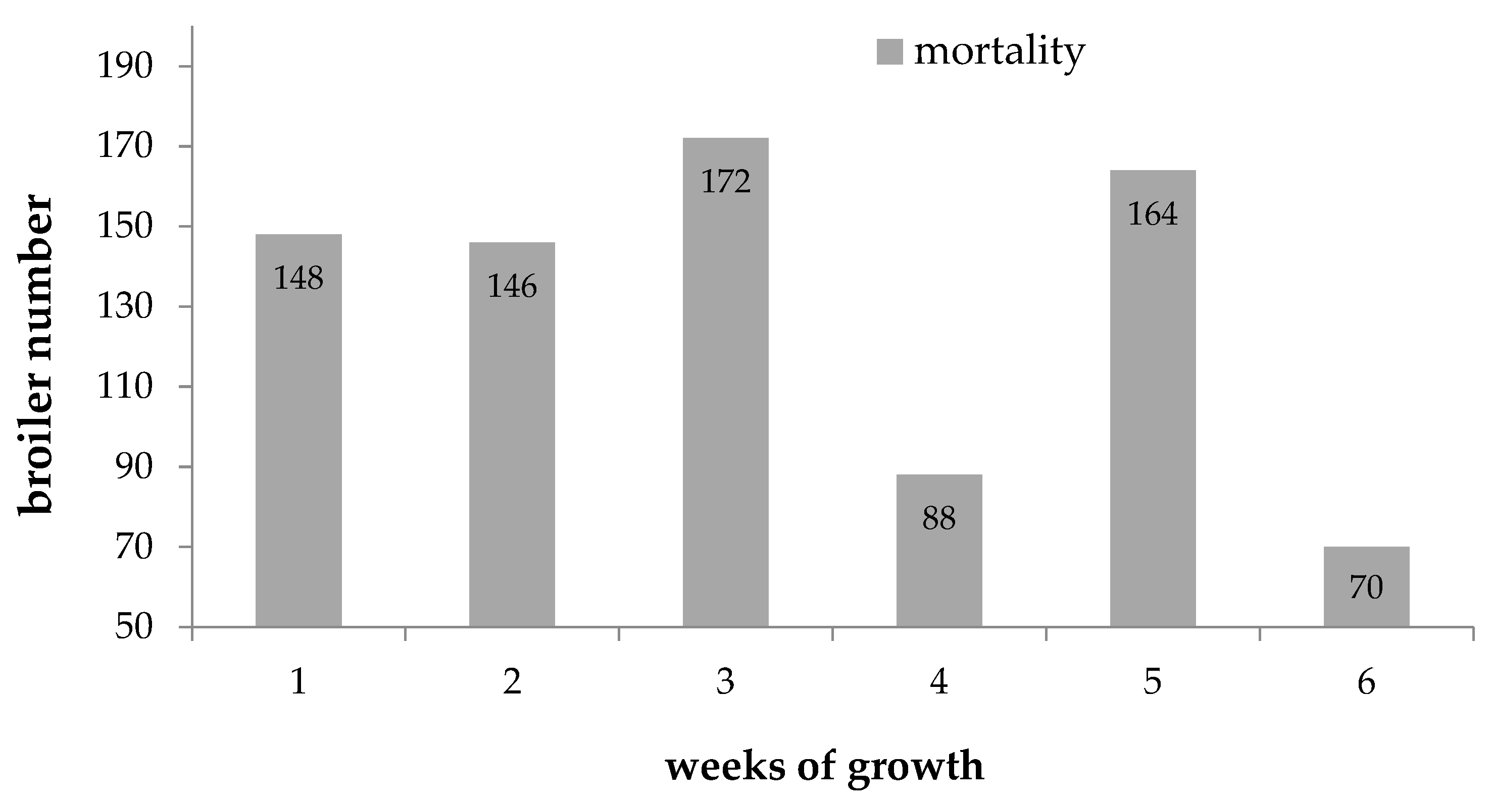
Monitoring and counting dead or discarded birds are crucial for identifying management and health issues, ensuring production efficiency, and improving profitability and animal welfare. For this production cycle, the weekly mortality is shown in Figure 17.

Figure 17.
Weekly count of mortality in number of broilers.
The first week of life of broiler chickens is critical for mortality and overall productivity, due to the transition that affects chick survival being influenced by management practices and housing conditions [73].
Increased mortality is associated with floor quality, neonatal septicemia, ventilation type, and producer management conditions [74]. Although some weeks experienced environments outside of the ideal thermal comfort conditions, the mortality rate observed during this production cycle is considered low.
Technological failures in the management of the dark-house system can also cause environmental contamination, resulting in carcass condemnations at pre-slaughter due to conditions such as ascitic syndrome, hemorrhagic syndrome, arthritis, cachexia, and others [75]. However, if well managed, the dark-house system brings benefits in the reduction of thermal stress, controlling lighting, and feed conversion [57,76].
4. Study Constraints and Functional Impacts
This study focused on a single type of poultry house, analyzing how the control of thermal variables affects animal performance. While the short-term impact has been highlighted, a more comprehensive view can be obtained by considering a longer evaluation period, including seasonal variations. Comparing different closure materials in dark-house systems could yield valuable regional insights, as well as incorporate factors such as ventilation. However, biosecurity restrictions in commercial broiler production present significant challenges for expanding research. Additionally, installing more sensors to achieve greater spatial variability, while important for improving data accuracy, may considerably increase costs, making the process more burdensome.
The study underscores the importance of the continuous monitoring of thermal variables and frequent adjustments in management, utilizing indices such as THI, BGHI, or enthalpy. The choice of an appropriate index to assess the environment facilitates efficient adjustments in ventilation, heating, or cooling practices, promoting a conducive environment for their growth and performance.
5. Conclusions
Continuously monitoring and adjusting the environmental conditions in poultry houses is crucial for achieving the ideal thermal comfort needed for efficient broiler production. The dark-house system is designed to optimize environmental variables for the birds’ development, but it requires proper management and scheduling for each week of life and different regions of the country.
The first week of production and the period from the sixth week are critical. The first week is significant due to the transition of the chicks to their new environment, while from the sixth week onwards, the increased body mass of the birds raises the ambient temperature.
The spatial variability by region allowed the characterization of the magnitude of temperature and relative humidity, as well as thermal indices such as THI, BGHI, and H. The spatial analysis of these variables and indices highlights the need to correct the microclimate and maintain homogeneity to ensure optimal thermal comfort conditions in poultry production.
This study underscores the need for a scientific and technological approach to enhance the environmental management practices in poultry production systems.
Author Contributions
Conceptualization, J.C.F., M.B. and P.F.P.F.; methodology, J.C.F., A.T.C., T.Y.J., J.P.d.S. and S.C.F.; formal analysis, J.C.F. and M.B.; investigation, J.C.F., M.B. and P.F.P.F.; resources, J.C.F., A.T.C., J.P.d.S. and S.C.F.; data curation, J.C.F. and M.B.; writing—original draft preparation, J.C.F. and M.B.; writing—review and editing, J.C.F. and P.F.P.F.; visualization, S.C.F. and P.F.P.F.; supervision, A.T.C., T.Y.J. and J.P.d.S.; project administration, J.C.F. and A.T.C.; funding acquisition, A.T.C. All authors have read and agreed to the published version of the manuscript.
Funding
This study was financed in part by the National Council for Scientific and Technological Development (CNPq-131330/2015-2).
Data Availability Statement
Data are contained within the article.
Acknowledgments
We appreciate the support of the company Atalaia in the installation of the data acquisition system.
Conflicts of Interest
The authors declare no conflicts of interest.
References
- Associação Brasileira de Proteína Animal (ABPA). Relatório Anual 2024; ABPA: São Paulo, Brazil, 2024; Available online: https://abpa-br.org/wp-content/uploads/2024/04/ABPA-Relatorio-Anual-2024_capa_frango.pdf (accessed on 11 June 2024).
- Oliveira Júnior, A.J.; Sousa, G.S.; Dal Pai, E.; Almeida, O.C.P.; Mollo Neto, M.; Simões, R.P.; Lucas de Souza, S.R. System for assessing broilers thermal comfort. Smart Agric. Technol. 2021, 1, 100007. [Google Scholar] [CrossRef]
- Ribeiro, B.P.V.; Yanagi Junior, T.; de Oliveira, D.D.; de Lima, R.R.; Zangeronimo, M.G. Thermoneutral zone for laying hens based on environmental conditions, enthalpy and thermal comfort indexes. J. Therm. Biol. 2020, 93, 102678. [Google Scholar] [CrossRef]
- Medeiros, B.B.L.; Moura, D.J.; Massari, J.M.; Curi, T.M.R.C.; Maia, A.P.A. Uso de geoestatística na avaliação de variáveis ambientais em galpão de suínos criados em sistema “wean to finish” na fase de terminação. Eng. Agríc. 2014, 34, 800–811. [Google Scholar] [CrossRef]
- Garcia, R.G.; Lima, N.D.S.; Naas, I.A.; Caldara, F.R.; Sgavioli, S. The typology of broiler house and the impact in the locomotion of broilers. Eng. Agríc. 2018, 38, 326–333. [Google Scholar] [CrossRef]
- Pan, K.F.; Siqueira, J.A.C.; de Souza, S.N.M.; Tokura, L.K.; Nogueira, C.E.C.; Dieter, J.; Caneppele, F.L. Evaluation of broiler dark house illumination systems, with and without thermal insulation. Res. Soc. Dev. 2021, 10, e170101220155. [Google Scholar] [CrossRef]
- Curi, T.M.R.C.; Silva, A.M.; Lima, M.A.; Santos, D.M. Geoestatística para a avaliação do controle ambiental do sistema de ventilação em instalações comerciais para frangos de corte. Eng. Agríc. 2014, 34, 1062–1074. [Google Scholar] [CrossRef]
- Carvalho, T.M.R.; Ribeiro, J.F.; Oliveira, A.F. Qualidade da cama e do ar em diferentes condições de alojamento de frangos de corte. Pesq. Agropec. Bras. 2011, 46, 351–361. [Google Scholar] [CrossRef]
- Liu, L.; Ren, M.; Ren, K.; Jin, Y.; Yan, M. Heat stress impacts on broiler performance: A systematic review and meta-analysis. Poult. Sci. 2020, 99, 6205–6211. [Google Scholar] [CrossRef]
- Andretta, I.; Kipper, M.; Schirmann, G.; Franceschina, C.; Ribeiro, A. Modeling the performance of broilers under heat stress. Poult. Sci. 2021, 100, 101338. [Google Scholar] [CrossRef]
- Wu, X.Y.; Wang, F.Y.; Chen, H.X.; Dong, H.L.; Zhao, Z.Q.; Si, L.F. Chronic heat stress induces lung injury in broiler chickens by disrupting the pulmonary blood-air barrier and activating TLRs/NF-κB signaling pathway. Poult. Sci. 2023, 102, 103066. [Google Scholar] [CrossRef]
- Saeed, M.; Abbas, G.; Alagawany, M.; Kamboh, A.A.; Abd El-Hack, M.E.; Khafaga, A.F.; Sun, C. Heat stress management in poultry farms: A comprehensive overview. J. Therm. Biol. 2019, 84, 414–425. [Google Scholar] [CrossRef] [PubMed]
- Skomorucha, I.; Sosnówka-Czajka, E. Effect of rearing technology on production performance, selected blood parameters, and welfare levels of broiler chickens during the summer production cycle. Ann. Anim. Sci. 2024, 24, 939–948. [Google Scholar] [CrossRef]
- Sumanu, V.O.; Naidoo, V.; Oosthuizen, M.C.; Chamunorwa, J.P. Adverse effects of heat stress during summer on broiler chickens production and antioxidant mitigating effects. Int. J. Biometeorol. 2022, 66, 2379–2393. [Google Scholar] [CrossRef] [PubMed]
- Omomowo, O.O.; Falayi, F.R. Temperature-Humidity Index and Thermal Comfort of Broilers in Humid Tropics. Agric. Eng. Int. CIGR J. 2021, 23, 101. Available online: http://www.cigrjournal.org (accessed on 11 June 2024).
- Rostagno, M.H. Effects of heat stress on the gut health of poultry. J. Anim. Sci. 2020, 98, skaa090. [Google Scholar] [CrossRef]
- El-Sabrout, K.; Sherasiya, A.; Ahmad, S.; Aggag, S.; Nannoni, E.; Cavallini, D.; Buonaiuto, G. Environmental Enrichment in Rabbit Husbandry: Comparative Impacts on Performance and Welfare. Animals 2024, 14, 2367. [Google Scholar] [CrossRef]
- Vastolo, A.; Serrapica, F.; Cavallini, D.; Fusaro, I.; Atzori, A.S.; Todaro, M. Editorial: Alternative and novel livestock feed: Reducing environmental impact. Front. Vet. Sci. 2024, 11, 1441905. [Google Scholar] [CrossRef]
- Felini, R.; Cavallini, D.; Buonaiuto, G.; Bordin, T. Assessing the impact of thermoregulatory mineral supplementation on thermal comfort in lactating Holstein cows. Vet. Anim. Sci. 2024, 24, 100363. [Google Scholar] [CrossRef]
- dos Santos Harada, É.; Montanhani ME, S.; de Freitas Bueno, L.G.; Neto, M.M.; de Souza SR, L.; da Fonseca, R. Árvores de decisão baseadas em entalpia para avaliação de conforto para poedeiras leves em clima tropical. Res. Soc. Dev. 2021, 10, e45310313354. [Google Scholar] [CrossRef]
- Jongbo, A.O.; Atta, A.T. State-of-the-art technologies for assessing thermal comfort of broiler chickens. Int. J. Eng. Appl. Sci. Technol. 2019, 4, 72–83. [Google Scholar] [CrossRef]
- Thom, E.C. The discomfort index. Weatherwise 1959, 12, 57–59. [Google Scholar] [CrossRef]
- Buffington, D.E.; Collasso-Arocho, A.; Canton, G.H. Black Globe-Humidity Index (BGHI) as Comfort Equation for Dairy Cows. Trans. ASAE 1981, 24, 711–714. [Google Scholar] [CrossRef]
- Rodrigues, V.C.; Silva, I.J.O.; Vieira, F.M.C.; Nascimento, S.T. A correct enthalpy relationship as thermal comfort index for livestock. Int. J. Biometeorol. 2010, 55, 455–459. [Google Scholar] [CrossRef] [PubMed]
- Pecoraro, C.A.; Gonçalves, J.C.; Nunes, E.H.; Bumbieris Junior, V.H.; Tavares Filho, J.; Miranda, K.O.S. Enthalpy as a thermal comfort index in broiler poultry production. Rev. Bras. Eng. Agric. Ambient. 2024, 28, e270399. [Google Scholar] [CrossRef]
- de Sá Júnior, A.; de Carvalho, L.G.; Da Silva, F.F.; de Carvalho Alves, M. Application of the Köppen classification for climatic zoning in the state of Minas Gerais, Brazil. Theor. Appl. Climatol. 2012, 108, 1–7. [Google Scholar] [CrossRef]
- Bachmaier, M.; Backes, M. Variogram or semivariogram? Understanding the variances in a variogram. Precis. Agric. 2008, 9, 173–175. [Google Scholar] [CrossRef]
- de Mello, C.R.; Viola, M.R. Mapeamento de chuvas intensas no estado de Minas Gerais. Rev. Bras. Ciênc. Solo 2013, 37, 37–44. [Google Scholar] [CrossRef]
- Cambardella, C.A.; Moorman, T.B.; Novak, J.M.; Parkin, T.B.; Karlen, D.L.; Turco, R.F.; Konopka, A.E. Field scale variability of soil properties in Central Iowa soils. Soil Sci. Soc. Am. J. 1994, 58, 1501–1511. [Google Scholar] [CrossRef]
- Faustino, A.C.; Turco, S.H.N.; Silva Junior, R.G.C.; Miranda, I.B.; Anjos, I.E.; Lourençoni, D. Variabilidade espacial da entalpia e da iluminância em galpões de frangos caipiras. Rev. Bras. Eng. Agríc. Ambient. 2021, 25, 340–344. [Google Scholar] [CrossRef]
- Guesine, G.D.; Silveira, R.M.F.; Silva, I.J.O. Spatial modeling via geostatistics of the bed in a compost barn system: Thermal performance assessments. Int. J. Biometeorol. 2023, 67, 1775–1788. [Google Scholar] [CrossRef]
- Bournet, P.E.; Boulard, T. Effect of ventilator configuration on the distributed climate of greenhouses: A review of experimental and CFD studies. Comput. Electron. Agric. 2010, 74, 195–217. [Google Scholar] [CrossRef]
- Xue, Z.; Fang, X.; Wang, W.; An, S. Soil Organic Carbon Distribution Under Different Land Uses and Landscape Positions in Two Typical Watersheds of the Loess Plateau, China. Nat. Environ. Pollut. Technol. 2014, 13, 693–700. [Google Scholar]
- Infantino, M.; Smerzini, C.; Lin, J. Spatial Correlation of Broadband Ground Motions from Physics-Based Numerical Simulations. Earthq. Eng. Struct. Dyn. 2021, 50, 2575–2594. [Google Scholar] [CrossRef]
- Szatmári, G.; Pásztor, L.; Heuvelink, G.B.M. Estimating Soil Organic Carbon Stock Change at Multiple Scales Using Machine Learning and Multivariate Geostatistics. Geoderma 2021, 403, 115356. [Google Scholar] [CrossRef]
- Oliveira, C.E.A.; Tinôco, I.D.F.F.; de Oliveira, V.C.; Rodrigues, P.H.D.M.; Silva, L.F.D.; Damasceno, F.A.; Andrade, R.R.; Sousa, F.C.D.; Barbari, M.; Bambi, G. Spatial Distribution of Bedding Attributes in an Open Compost-Bedded Pack Barn System with Positive Pressure Ventilation in Brazilian Winter Conditions. Animals 2023, 13, 786. [Google Scholar] [CrossRef]
- Valente, G.F.; Ferraz, G.A.E.S.; Santana, L.S.; Ferraz, P.F.P.; Mariano, D.D.C.; Dos Santos, C.M.; Okumura, R.S.; Simonini, S.; Barbari, M.; Rossi, G. Mapping Soil and Pasture Attributes for Buffalo Management through Remote Sensing and Geostatistics in Amazon Biome. Animals 2022, 12, 2374. [Google Scholar] [CrossRef]
- Silva, M.A.J.G.; Ferraz, P.F.P.; Santos, L.M.D.; Ferraz, G.A.E.S.; Rossi, G.; Barbari, M. Effect of the Spatial Distribution of the Temperature and Humidity Index in a New Zealand White Rabbit House on Respiratory Frequency and Ear Surface Temperature. Animals 2021, 11, 1657. [Google Scholar] [CrossRef]
- Ferraz, P.F.P.; Ferraz, G.A.S.; Schiassi, L.; Nogueira, V.H.B.; Barbari, M.; Damasceno, F.A. Spatial variability of litter temperature, relative air humidity and skin temperature of chicks in a commercial broiler house. Agron. Res. 2019, 17, 408–417. [Google Scholar] [CrossRef]
- Silva, R.A.; Siqueira, G.M.; Costa, M.K.L.; Guedes Filho, O.; Silva, Ê.F.F. Spatial Variability of Soil Fauna Under Different Land Use and Managements. Rev. Bras. Ciênc. Solo 2018, 42, e0170121. [Google Scholar] [CrossRef]
- Guedes, L.P.C.; Bach, R.T.; Uribe-Opazo, M.A. Nugget Effect Influence on Spatial Variability of Agricultural Data. Eng. Agríc. 2020, 40, 96–104. [Google Scholar] [CrossRef]
- Seidel, E.; Oliveira, M. Uma classificação para um índice geoestatístico de dependência espacial. Rev. Bras. Ciênc. Solo 2016, 40, e0160007. [Google Scholar] [CrossRef]
- Silva, I.M.; Pandorfi, H.; Almeida, G.L.P.; Guiselini, C.; Caldas, A.M.; Jacob, A.L. Análise espacial das condições térmicas do ambiente pré-ordenha de bovinos leiteiros sob regimes de climatização. Rev. Bras. Eng. Agríc. Ambient. 2012, 16, 903–909. [Google Scholar] [CrossRef]
- Santos, C.; Matsunaga, A.; Costa, L.; Santos, M.; Neto, A.; Rodrigues, R.; Melo, V. Variabilidade espacial da fertilidade do solo sob sistema agroflorestal e floresta nativa na Amazônia oriental, Brasil. Biosci. J. 2023, 39, e39015. [Google Scholar] [CrossRef]
- Küçüktopcu, E.; Cemek, B. Modelling indoor environmental conditions in a commercial broiler house. J. Agric. Sci. 2019, 25, 440–448. [Google Scholar] [CrossRef]
- Ferraz, P.F.P.; Yanagi Junior, T.; Ferraz, G.A.S.; Schiassi, L.; Campos, A.T. Variabilidade Espacial da Entalpia em Galpões Avícolas na Fase de Aquecimento. Rev. Bras. Eng. Agríc. Ambient. 2016, 20, 570–575. [Google Scholar] [CrossRef]
- Carvalho, T.M.R.; Moura, D.J.; Souza, Z.M.; Souza, G.S.; Bueno, L.G.F.; Lima, K.A.O. Use of Geostatistics on Broiler Production for Evaluation of Different Minimum Ventilation Systems During Brooding Phase. Rev. Bras. Zootec. 2012, 41, 194–202. [Google Scholar] [CrossRef]
- Santos, M.P.; Deniz, M.; Tenffen de Sousa, K.; Klein, D.R.; Branco, T.; Pacheco, P.S.; Martinez do Vale, M. Efficiency of Cooling Systems in Broiler Houses During Hot Days. Ciênc. Rural 2021, 51, e20200941. [Google Scholar] [CrossRef]
- Lopes, I.; da Silva, M.V.; de Melo, J.M.M.; de, A. Montenegro, A.A.; Pandorfi, H. Geostatistics Applied to the Environmental Mapping of Aviaries. Rev. Bras. Eng. Agríc. Ambient. 2020, 24, 409–414. [Google Scholar] [CrossRef]
- Tedeschi, L.O. Assessment of the Adequacy of Mathematical Models. Agric. Syst. 2006, 89, 225–247. [Google Scholar] [CrossRef]
- Medeiros, C.M.; Baêta, F.C.; Oliveira, R.F.M.; Tinôco, I.F.F.; Albino, L.F.T.; Cecon, P.R. Efeitos da Temperatura, Umidade Relativa e Velocidade do Ar em Frangos de Corte. Eng. Agric. 2005, 13, 277–286. [Google Scholar]
- Ferraz, P.F.P.; Yanagi Junior, T.; Ferraz, G.A.S.; Damasceno, F.A. Distribuição Espacial do Índice de Temperatura do Globo e Umidade em Galpão de Frangos na Primeira Semana de Vida Aquecido por Fornalha Industrial. Energ. Agric. 2017, 32, 356–363. [Google Scholar] [CrossRef]
- Abreu, L.H.P.; Yanagi, T.; Bahuti, M.; Lima, R.R.; Lourençoni, D.; Fassani, É.J. Performance of Broilers Submitted to Different Intensities and Duration of Thermal Stress. Dyna 2019, 86, 131–137. [Google Scholar] [CrossRef]
- Soliman, A.; Safwat, A.M. Climate Change Impact on Immune Status and Productivity of Poultry as Well as the Quality of Meat and Egg Products. In Climate Change Impacts on Agriculture and Food Security in Egypt; Omran, E.-S.E., Negm, A.M., Eds.; Springer Water: Berlin/Heidelberg, Germany, 2020; pp. 1–12. [Google Scholar] [CrossRef]
- Aviagen. Ross Manual de Manejo de Frangos de Corte; Aviagen: Huntsville, AL, USA, 2018. [Google Scholar]
- Apalowo, O.O.; Ekunseitan, D.A.; Fasina, Y.O. Impact of Heat Stress on Broiler Chicken Production. Poultry 2024, 3, 107–128. [Google Scholar] [CrossRef]
- Lourençoni, D.; Yanagi Junior, T.; Abreu, P.G.D.; Campos, A.T.; Yanagi, S.D.N. Productive Responses from Broiler Chickens Raised in Different Commercial Production Systems—Part I: Fuzzy Modeling. Eng. Agríc. 2019, 39, 1–10. [Google Scholar] [CrossRef]
- Ponciano, P.F.; Yanagi Junior, T.; Schiassi, L.; Campos, A.T.; Nascimento, J.W.B. Sistema fuzzy para predição do desempenho produtivo de frangos de corte de 1 a 21 dias de idade. Eng. Agríc. 2012, 32, 446–458. [Google Scholar] [CrossRef]
- Cândido, M.G.; Tinôco, I.D.F.; Pinto, F.D.A.D.C.; Santos, N.T.; Roberti, R.P. Determination of thermal comfort zone for early-stage broilers. Eng. Agríc. 2016, 36, 760–767. [Google Scholar] [CrossRef]
- Silva, E.T.; Leite, D.G.; Yuri, F.M.; Nery, F.S.G.; Rego, J.C.C.; Zanatta, R.A.; dos Santos, S.A.; Moura, V.V. Determinação do índice de temperatura e umidade (ITU) para produção de aves na mesorregião metropolitana de Curitiba—PR. Rev. Acad. Ciênc. Agrár. Ambient. 2004, 2, 47–60. [Google Scholar] [CrossRef]
- Furtado, D.A.; Dantas, R.T.; Nascimento, J.W.B.; Santos, J.T.; Costa, F.G.P. Efeitos de diferentes sistemas de acondicionamento ambiente sobre o desempenho produtivo de frangos de corte. Rev. Bras. Eng. Agríc. Ambient. 2006, 10, 484–489. [Google Scholar] [CrossRef]
- Ferraz, P.F.P.; Yanagi Junior, T.; Melo, L.F.L.D.; Castro, J.D.O.; Cecchin, D. Spatial and temporal distribution of enthalpy in aviary heated by industrial furnace. Rev. Ceres 2018, 65, 346–355. [Google Scholar] [CrossRef][Green Version]
- Martinez, A.A.G.; Nääs, I.D.A.; Abe, J.M.; Pereira, D.F. A Mobile Application to Follow Up the Management of Broiler Flocks. AgriEngineering 2021, 3, 990–1000. [Google Scholar] [CrossRef]
- Silva, R.B.T.R.; de Nääs, I.A.; de Oliveira Júnior, A.J.; dos Reis, J.G.M.; Lima, N.D.D.S.; de Souza, S.R.L. Improving the Management of Poultry Production: Mobile Application Development and Validation. Res. Soc. Dev. 2020, 9, e4019108806. [Google Scholar] [CrossRef]
- Wasti, S.; Sah, N.; Mishra, B. Impact of Heat Stress on Poultry Health and Performances, and Potential Mitigation Strategies. Animals 2020, 10, 1266. [Google Scholar] [CrossRef] [PubMed]
- Barbosa Filho, J.A.D.; Vieira, F.M.C.; Garcia, D.B.; Silva, M.A.N.; Silva, I.J.O. Mudanças e uso das Tabelas de Entalpia; Piracicaba: São Paulo, Brazil, 2007; Available online: http://www.nupea.esalq.usp.br/ (accessed on 5 June 2024).
- Moghadam, A.; Thippareddi, H.; Pidaparti, R. Machine Learning Model for Assuring Bird Welfare during Transportation. AgriEngineering 2022, 4, 367–379. [Google Scholar] [CrossRef]
- Queiroz, M.L.V.; Barbosa Filho, J.A.D.; Sales, F.A.L.; Lima, L.R.; Duarte, L.M. Variabilidade Especial do Ambiente em Galpões de Frango de Corte com Sistema de Nebulização. Ciênc. Agron. 2017, 48, 586–595. Available online: https://www.scielo.br/j/rca/a/9p9TyxyY7zvD8zXWLxynM6K/?format=pdf&lang=pt (accessed on 5 June 2024).
- Gonçalves, I.C.M.; Turco, S.H.N.; Lopes Neto, J.P.; Nascimento, J.W.B.; Lima, V.L.A.; Borges, V.P. Thermal Performance of Aviary Located in the Semiarid Region of Pernambuco Based on Computer Simulation. Rev. Bras. Eng. Agríc. Ambient. 2022, 26, 533–540. [Google Scholar] [CrossRef]
- Brito, A.N.S.L.; Lopes Neto, J.P.; Furtado, D.A.; Mascarenhas, N.M.H.; Oliveira, A.G.; Gregório, M.G.; Dornelas, K.C.; Laurentino, L.G.S.; Rodrigues, H.C.S. Desempenho Térmico de Galpões Avícolas para Frangos de Corte: Revisão Sobre os Diferentes Tipos de Coberturas. Res. Soc. Dev. 2020, 9, e474997608. [Google Scholar] [CrossRef]
- Cobb-Vantress. Cobb500TM Suplemento de Nutrição e Desempenho do Frango de Corte; CobbCares: Siloam Springs, AR, USA, 2022; Available online: https://www.cobbgenetics.com/assets/Cobb-Files/2022-Cobb500-Broiler-Performance-Nutrition-Supplement.pdf (accessed on 5 June 2024).
- Rubio, A.A.; Hess, J.B.; Berry, W.D.; Dozier, W.A.; Pacheco, W.J. Effects of Corn Particle Size on Broiler Performance During the Starter, Grower, and Finisher Periods. J. Appl. Poult. Res. 2020, 29, 352–361. [Google Scholar] [CrossRef]
- Yerpes, M.; Llonch, P.; Manteca, X. Factors Associated with Cumulative First-Week Mortality in Broiler Chicks. Animals 2020, 10, 310. [Google Scholar] [CrossRef]
- Van Limbergen, T.; Sarrazin, S.; Chantziaras, I.; Dewulf, J.; Ducatelle, R.; Kyriazakis, I.; McMullin, P.; Méndez, J.; Niemi, J.K.; Papasolomontos, S.; et al. Risk factors for poor health and performance in European broiler production systems. BMC Vet. Res. 2020, 16, 287. [Google Scholar] [CrossRef]
- Santos, G.R.; Reati, L.A.; Dias, E.H.; Dorneles, I.C.; Mezalira, T.S.; Otutumi, L.K. Percentage of Condemnations of Broiler Carcasses Related to Lineage and Breeding System. Ciênc. Anim. 2019, 29, 12–21. Available online: https://revistas.uece.br/index.php/cienciaanimal/article/view/9889 (accessed on 5 June 2024).
- Ozkan, M.; Simsek, U.G. The effect of light/dark cycles on performance and welfare in broiler. Ann. Anim. Sci. 2022, 22, 795–802. [Google Scholar] [CrossRef]
Disclaimer/Publisher’s Note: The statements, opinions and data contained in all publications are solely those of the individual author(s) and contributor(s) and not of MDPI and/or the editor(s). MDPI and/or the editor(s) disclaim responsibility for any injury to people or property resulting from any ideas, methods, instructions or products referred to in the content. |
© 2024 by the authors. Licensee MDPI, Basel, Switzerland. This article is an open access article distributed under the terms and conditions of the Creative Commons Attribution (CC BY) license (https://creativecommons.org/licenses/by/4.0/).

