Regional Sensitivity Analysis of Slope Stability in Weathered Marly Soils: Parameter Ranking and Threshold Robustness at Moulay Yacoub, Morocco

Abstract

Weathered marl hillslopes fail repeatedly across peri-urban Morocco, yet engineers investigating them rarely know which soil or geometric property most deserves their limited testing budget. This study answers that question for the landslide-prone slopes of Moulay Yacoub, in the northern pre-Rifian domain, by ranking the sensitivity of the factor of safety (FoS) to cohesion (c), friction angle (φ), unit weight (γ), slope height (H) and slope angle (β) under dry, deep-water-table conditions. Latin hypercube sampling generated 400 configurations over ranges drawn from site data; the FoS of each was computed by Bishop’s simplified method in Talren, and regional sensitivity analysis—the two-sample Kolmogorov–Smirnov statistic with a relative sensitivity index—ranked the five inputs. Cohesion governs the response by a wide margin (D = 0.470; 38.2% of total sensitivity at FoS = 1.2), ahead of slope height and friction angle (D ≈ 0.26); slope angle is marginal, and unit weight is not discriminating. Repeating the analysis at four thresholds (1.1–1.4) shows that the primacy of cohesion is threshold-independent, and that the apparent significance of slope angle at stricter thresholds is a statistical power effect, not a mechanical one. Site investigation in comparable marl settings should prioritise cohesion characterisation.

1. Introduction

Landslides are among the most damaging and frequent natural hazards worldwide [1], and are particularly frequent where weak or weathered formations crop out in steep terrain subject to intense rainfall [2]. Among the materials most susceptible to instability, weathered marls hold a distinct place: their mechanical response depends heavily on the degree of weathering and on water content, which is why they rank among the most challenging materials in slope engineering [3].

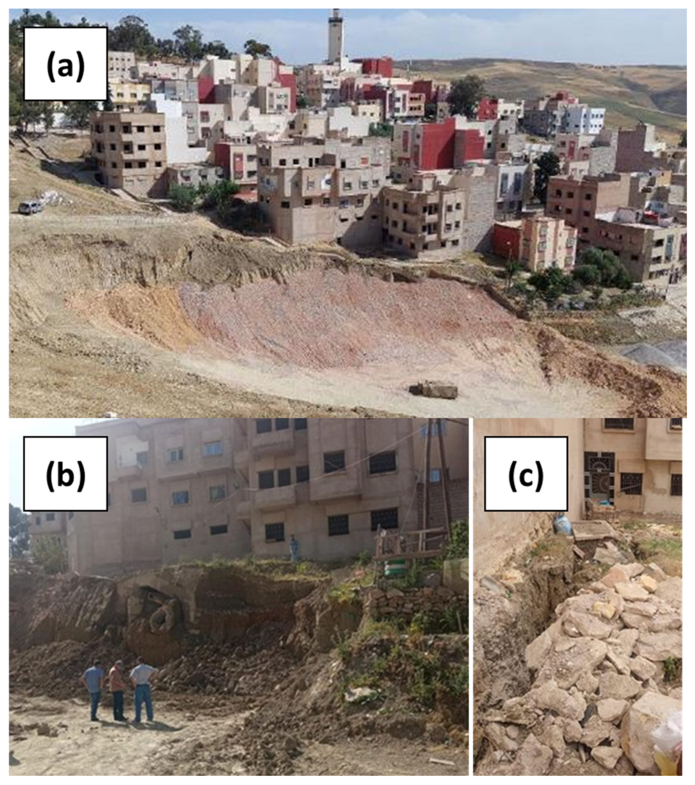
The province of Moulay Yacoub, in the peri-urban hinterland north-west of Fez, Morocco, highlights the problem. Its hillslopes are cut into a thick sequence of Miocene marls whose mechanical properties evolve with weathering, and population growth has pushed construction onto steep slopes, increasing exposure [4,5]. At Moulay Yacoub, these movements are predominantly shallow and slow-moving, developing within the weathered surface mantle rather than as deep, abrupt failures [4], repeatedly damaging housing, retaining structures and roads; comparable instabilities recur along strategic corridors elsewhere in the Moroccan Rif, such as the deep-seated landslide affecting National Road 16 [6]. These instabilities are documented by field surveys carried out by the LPEE (Laboratoire Public d’Essais et d’Études) (Figure 1): low-rise buildings stand immediately behind slopes cut into the weathered marl (Figure 1a), and the movements are closely associated with unsupported vertical excavations at the toe, from which failure propagates upslope towards the housing (Figure 1b). Open ground fractures and escarpments of several tens of centimetres, together with tilted structures, mark the affected ground at the foot of the buildings (Figure 1c).

This recurrence motivates a quantitative understanding of which parameters actually govern slope stability in this geological context.

Geologically, the town lies in the Neogene South-Rifian corridor at its contact with the Pre-Rif domain—the Rif being the mountain belt of northern Morocco, and the Pre-Rif its southern foreland—a subsiding basin dominated by Upper Miocene marls; the Tortonian–Messinian marls form the bulk of the hillslopes on which the town is built and constitute the layer analysed in the present study [4,7]. These peri-Mediterranean Neogene marly soils are recognised for their tendency to swell, shrink and disperse, and for their persistent instability [8,9,10,11].

Slope stability analysis classically relies on limit equilibrium methods (LEM), which assume the failure geometry a priori and solve the equilibrium of a set of slices [12]; finite element strength-reduction approaches avoid this assumption at higher cost [13]. Beyond computing a factor of safety for a given model, understanding slope stability increasingly requires quantifying which inputs most influence the response—the purpose of sensitivity analysis [14]. Existing sensitivity studies of the factor of safety generally rank the shear strength parameters first, followed by slope geometry [15,16,17,18,19].

A recent review concludes that, among the geotechnical inputs, cohesion emerges as the critical factor governing computed stability [20]; modelling the factor of safety of rock slopes from the same five inputs used here, Trinidad and Momayez [21] reach the same hierarchy, with unit weight the least influential. The convergence with soil-nail-reinforced slopes, where cohesion, friction angle and slope inclination likewise control local instability [22], reinforces the point.

Global and regional sensitivity analysis frameworks rank the inputs of a slope-stability model and, for regional methods, map the regions of the input space associated with instability, identifying where characterisation effort will most reduce predictive uncertainty [23,24]. They have been applied to cohesive-frictional soils [15], residual soils [25] and rock slopes [16], and probabilistic approaches coupled with machine learning have propagated shear strength variability into failure probabilities [26], while neural-network models have been developed to predict the failure stresses and strains of cohesive soils [27]. Few studies, however, address weathered marly soils, and none, to the authors’ knowledge, in the Moulay Yacoub region.

Beyond variance- and density-based frameworks, machine learning is increasingly used to emulate slope-stability models and propagate parameter uncertainty. Physics-informed surrogate models that embed Mohr–Coulomb features reproduce factor-of-safety distributions and reliability estimates from limited numerical runs, including Latin-hypercube designs [28]. At the regional scale, transfer-learning approaches address a difficulty directly relevant here—the limited transferability of a model calibrated in one setting to geologically different terrain—by quantifying source–target similarity before knowledge transfer [29] and by extrapolating landslide susceptibility across regions [30]. These methods require a trained predictor or a spatial inventory; the present study is complementary and prior to them, performing a model-free ranking that identifies which parameters a future surrogate or transfer-learning model should prioritise in this lithological context.

This study ranks the influence of cohesion c, friction angle φ, unit weight γ, slope height H and slope angle β on the factor of safety of weathered marl slopes under dry conditions, over ranges derived from LPEE’s site investigation data. Latin hypercube sampling (LHS) generates 400 slope configurations, whose factors of safety are computed with Bishop’s simplified method; regional sensitivity analysis (RSA) then ranks the parameters.

The study is deliberately confined to these geotechnical and geometric parameters: water-table depth and pore-pressure effects are excluded and are the object of a companion study. Establishing the soil and geometry controls under dry conditions first provides the baseline against which the hydraulic contribution can subsequently be isolated.

Two gaps motivate this work. First, although shear-strength parameters are repeatedly reported as dominant, sensitivity rankings are conditional on parameter ranges and on the behavioural threshold, and no published ranking exists for weathered pre-Rifian marls. Second, that threshold, on which every regional sensitivity ranking depends, is almost never tested. This study addresses both. Its contributions are: (i) the first regional sensitivity ranking of FoS controls for weathered pre-Rifian marls, over ranges derived from site data; (ii) an explicit threshold-robustness protocol at four thresholds (FoS = 1.1–1.4), separating threshold-independent conclusions from artefacts; and (iii) an actionable site-investigation product—the cohesion band over which stable and unstable slopes separate most strongly.

The restriction to dry, deep-water-table conditions is a deliberate staging choice. Water influences marly slopes via two mechanisms: it lowers the strength parameters by softening the weathered mantle, and it decreases effective stress through pore water pressure. The first is partially internalised in the present design, since the low end of the cohesion range corresponds to softened, moisture-affected states of the marl; the second is excluded and is the object of a companion study adding a variable phreatic surface to the same parametric framework. Ranking the geomechanical and geometric parameters alone first establishes the baseline against which the hydraulic contribution can then be isolated—a single design including both would confound them.

2. Materials and Methods

2.1. Failure Criterion and Factor of Safety

Slope stability analyses in cohesive-frictional materials rest on the Mohr–Coulomb criterion [31]:

$$\mathsf{\tau }={\mathrm{c}}^{\prime }+{\mathsf{\sigma }}^{\prime }\mathrm{t}\mathrm{a}\mathrm{n}{\mathrm{\phi }}^{\prime }$$

(1)

where τ is the shear strength (kPa), c′ the effective cohesion (kPa), σ′ the effective normal stress (kPa) and φ′ the effective friction angle (°). In weathered marls, c′ and φ′ vary strongly with the degree of weathering, moisture content and smectite content [3,32]. The factor of safety is the ratio of the available shear strength to the shear stress required for equilibrium along the slip surface [12]:

$$\mathrm{F}={\displaystyle \frac{{\mathrm{c}}^{\prime }+{\mathsf{\sigma }}^{\prime }\mathrm{t}\mathrm{a}\mathrm{n}{\mathrm{\phi }}^{\prime }}{{\mathsf{\tau }}_{\mathrm{e}\mathrm{q}}}}$$

(2)

Because the unknowns outnumber the equilibrium equations, LEM formulations differ in their simplifying assumptions [12].

2.2. Bishop’s Simplified Method

Bishop’s simplified method satisfies moment and vertical force equilibrium, suits the predominantly circular rotational slip surfaces observed in weathered materials, and matches more rigorous formulations for circular surfaces at a lower computational cost [33,34]. Assuming that the resultant of the interslice vertical forces vanishes for each slice:

$${\mathrm{F}}_{\mathrm{s}}={\displaystyle \frac{1}{{\displaystyle {\sum }_{\mathrm{n}=1}^{\mathrm{m}}}{\mathrm{W}}_{\mathrm{n}}\mathrm{s}\mathrm{i}\mathrm{n}{\mathsf{\alpha }}_{\mathrm{n}}}}\hspace{0.33em}{\displaystyle \sum _{\mathrm{n}=1}^{\mathrm{m}}}\hspace{0.33em}{\displaystyle \frac{{\mathrm{c}}^{\prime }\hspace{0.17em}{\mathrm{b}}_{\mathrm{n}}+\left({\mathrm{W}}_{\mathrm{n}}-{\mathrm{u}}_{\mathrm{n}}{\mathrm{b}}_{\mathrm{n}}\right)\mathrm{t}\mathrm{a}\mathrm{n}{\mathrm{\phi }}^{\prime }}{\mathrm{c}\mathrm{o}\mathrm{s}{\mathsf{\alpha }}_{\mathrm{n}}+\frac{\mathrm{s}\mathrm{i}\mathrm{n}{\mathsf{\alpha }}_{\mathrm{n}}\hspace{0.17em}\mathrm{t}\mathrm{a}\mathrm{n}{\mathrm{\phi }}^{\prime }}{{\mathrm{F}}_{\mathrm{s}}}}}$$

(3)

where W_n is the weight of slice n, b_n its width, α_n the inclination of its base, and u_n the pore water pressure at its base. Equation (3) is implicit in F_s and is solved by successive iterations, the first iteration adopting the Fellenius value as an initial estimate:

$${\mathrm{F}}_{\mathrm{s},0}={\displaystyle \frac{{\displaystyle {\sum }_{\mathrm{n}=1}^{\mathrm{m}}}\left(\frac{{\mathrm{c}}^{\prime }\hspace{0.17em}{\mathrm{b}}_{\mathrm{n}}}{\mathrm{c}\mathrm{o}\mathrm{s}{\mathsf{\alpha }}_{\mathrm{n}}}+{\mathrm{W}}_{\mathrm{n}}\mathrm{c}\mathrm{o}\mathrm{s}{\mathsf{\alpha }}_{\mathrm{n}}\mathrm{t}\mathrm{a}\mathrm{n}{\mathrm{\phi }}^{\prime }\right)}{{\displaystyle {\sum }_{\mathrm{n}=1}^{\mathrm{m}}}{\mathrm{W}}_{\mathrm{n}}\mathrm{s}\mathrm{i}\mathrm{n}{\mathsf{\alpha }}_{\mathrm{n}}}}$$

(4)

All analyses reported here are drained and assume a deep water table, so that u_n = 0 throughout.

2.3. Slope Model and Input Parameters

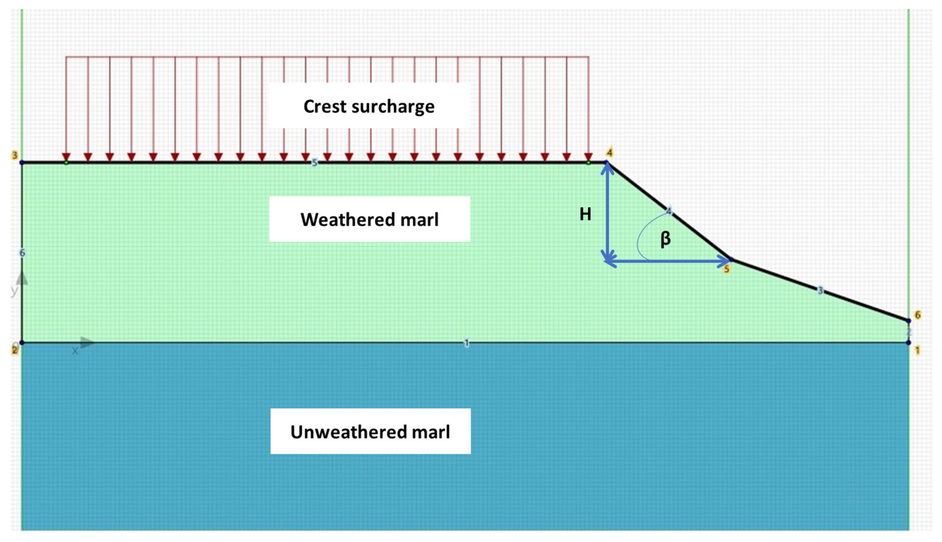
The simplified theoretical cross-section of the slope model implemented in Talren v6 (version 6.2.18; Terrasol) is shown in Figure 2.

The sliding layer is a single, homogeneous weathered marl unit characterised by its cohesion (c), friction angle (φ) and unit weight (γ). The slope is described by its height (H) and its angle (β). A distributed surcharge of 20 kN/m², representing the load of the adjacent buildings, is applied at the crest. This value is the mean characteristic load of the low-rise masonry buildings adjacent to the affected slopes (ground floor to two upper storeys, R to R + 2), whose usual loads span approximately 10–30 kN/m²; it was adopted on the basis of expert geotechnical judgement for the site. It is held constant rather than sampled because it represents a fixed exposure condition rather than an uncertain soil property.

Parameter ranges (

Table 1. Ranges of variation in the model parameters.

Parameter	Cohesion, c (kPa)	Friction Angle, φ (°)	Unit Weight, γ (kN/m3)	Height, H (m)	Slope Angle, β (°)
Range	5–50	8–25	18–22	3–15	25–70

) were set from previous geotechnical investigations and laboratory tests carried out in Moulay Yacoub. Throughout, c and φ denote the effective shear strength parameters (c′, φ′) of the drained analyses; the prime is dropped for brevity. Cohesion of the weathered marl in its various states lies between 5 and 50 kPa, friction angle between 8 and 25°, and unit weight between 18 and 22 kN/m³. The 5–50 kPa range covers the weathering profile of the Tortonian–Messinian marl, extending from the highly weathered, softened mantle at the lower limit to the slightly weathered marl near the upper limit that preserves some of its cementation bonds. It remains within soil-like behaviour and does not extend to the indurated marlstone of the unweathered substratum, whose effective cohesion is an order of magnitude higher. Because the slope movements documented at the site develop within this weathered mantle, whose degree of weathering—and hence cohesion—varies laterally and with depth across the affected hillslopes, the full interval is retained rather than truncated to a single weathering state. Slope angles and heights were assigned wide ranges to reflect anthropogenic disturbance in the area, in particular unsupported vertical or inclined excavations, so that even extreme configurations are covered.

Each parameter was assigned a uniform marginal distribution over its range, and the five parameters were treated as mutually independent. This is a deliberate screening assumption: in the absence of a paired c–φ dataset for the site, no correlation structure could be estimated, and imposing an arbitrary one would bias the ranking. The consequences of this assumption are discussed in Section 4.4.

2.4. Latin Hypercube Sampling

The input set was produced by Latin hypercube sampling (LHS), a stratified random sampling method introduced by McKay, Beckman, and Conover (1979) [35]. LHS partitions each input dimension into N equally probable intervals and draws one value per interval, so that every input is sampled across the full extent of its own range, including its marginal extremes. Stratification guarantees this marginal coverage; it does not guarantee coverage of joint extremes. This is relevant in geotechnical contexts, where instability can be governed by unfavourable combinations of parameter values.

For M input factors sampled in N strata, LHS produces an N × M sample matrix in which each row is one realisation; positions within each stratum are drawn by random permutation. The resulting design achieves variance reduction relative to simple random sampling, so that comparable sensitivity estimates are obtained with fewer simulations [36].

A total of N = 400 configurations were generated over the ranges of Table 1, a size chosen to keep the number of Talren computations tractable while holding the critical Kolmogorov–Smirnov value below 0.2 at every stability threshold considered in Section 2.6. The factor of safety of each configuration was computed in Talren using Bishop’s simplified method, the construction of the model and the extraction of the result being automated by a Python 3.12.3 script that reads each parameter set, writes it to the corresponding field in Talren, launches the computation and returns the FoS.

The search used circular surfaces in automatic mode, constrained to pass through a fixed base point at the slope toe, over a grid of centres swept above and behind the slope; the same search configuration was applied to every realisation, so that results are mutually comparable. All 400 factors of safety reported here were obtained under this single, uniformly applied search configuration. No pre-processing was applied beyond the LHS generation; realisations were classified as behavioural or non-behavioural solely on the recorded FoS relative to each threshold.

2.5. Regional Sensitivity Analysis

Sensitivity analysis measures how changes in input parameters influence and carry through to the model’s output [14]. Methods differ in the nature of the variability considered (local or global), the approach (qualitative or quantitative), the sampling strategy (one-at-a-time or all-at-once) and the objective (screening, ranking or mapping). Variance-based methods [37] support screening and ranking through the decomposition of output variance; density-based methods do so through changes in the probability density of the output.

Regional sensitivity analysis (RSA) was chosen here because the objective is both to rank the inputs and to identify the regions of the input space associated with instability—a combination that correlation- and regression-based approaches cannot deliver simultaneously [14]. RSA partitions the realisations into behavioural and non-behavioural sets with respect to a threshold on the output, and measures, for each input, the divergence between the empirical cumulative distribution functions (CDFs) of the two sets. The divergence is quantified by the two-sample Kolmogorov–Smirnov (KS) statistic:

$${\mathrm{D}}_{\mathrm{i}}=\underset{{\mathrm{x}}_{\mathrm{i}}}{\mathrm{s}\mathrm{u}\mathrm{p}}\left|{\mathrm{F}}_{{\mathrm{x}}_{\mathrm{i}}\mid \mathrm{B}}\left({\mathrm{x}}_{\mathrm{i}}\right)-{\mathrm{F}}_{{\mathrm{x}}_{\mathrm{i}}\mid \mathrm{B}\mathrm{c}}\left({\mathrm{x}}_{\mathrm{i}}\right)\right|$$

(5)

where ${\mathrm{F}}_{{\mathrm{x}}_{\mathrm{i}}\mid \mathrm{B}}$ and ${\mathrm{F}}_{{\mathrm{x}}_{\mathrm{i}}\mid \mathrm{B}\mathrm{c}}$ denote the empirical CDFs of input x_i restricted to the stable (behavioural) and unstable (non-behavioural) realisations. D_i is also known as the maximum vertical distance between the two CDFs.

To express each input’s share of the total sensitivity, the KS statistics are normalised into a relative sensitivity index:

$${\mathrm{R}\mathrm{S}\mathrm{I}}_{\mathrm{i}}={\displaystyle \frac{{\mathrm{D}}_{\mathrm{i}}}{{\displaystyle {\sum }_{\mathrm{j}=1}^{\mathrm{n}}}{\mathrm{D}}_{\mathrm{j}}}}\times 100$$

(6)

where n is the number of inputs. In this model-free setting, the RSI plays the role that feature-importance measures play for fitted predictive models, with the difference that it is computed directly on physically simulated outputs rather than on a surrogate approximation. Being computed on one input at a time, the KS statistic is a marginal (univariate) measure: it captures each input’s individual discriminating power but is blind to interaction effects, a property that must be kept in mind when interpreting low values [14]. Statistical significance was assessed with the two-sample KS test at α = 0.05; the corresponding critical value is ${\mathrm{D}}_{\mathrm{c}\mathrm{r}\mathrm{i}\mathrm{t}}\approx 1.36\sqrt{\left({\mathrm{n}}_{\mathrm{s}}+{\mathrm{n}}_{\mathrm{u}}\right)/\left({\mathrm{n}}_{\mathrm{s}}{\mathrm{n}}_{\mathrm{u}}\right)}$, where ns and nu are the sizes of the stable and unstable sets.

Because all statistics derive from a single LHS realisation, the sampling variability of each KS statistic was quantified by bootstrap: the 400 realisations were resampled with replacement 10,000 times and D recomputed for every input at the reference threshold, yielding 95% percentile confidence intervals. The analysis screens five inputs at four thresholds (20 KS tests) at an uncorrected α = 0.05; uncorrected significance is appropriate for exploratory ranking, and its robustness was checked against a conservative Bonferroni threshold (α = 0.0025).

2.6. Threshold Robustness Protocol

The classification of a realisation as behavioural or non-behavioural depends on the threshold applied to the factor of safety. To test whether the resulting ranking is an artefact of that choice, the RSA was repeated on the same 400 simulations at four thresholds: FoS = 1.1, 1.2, 1.3 and 1.4. This spans the range of values commonly adopted in slope design practice and, because the simulations are reused, isolates the effect of the threshold from any sampling variability. The threshold FoS = 1.2 is retained as the reference case in Section 3.1, Section 3.2 and Section 3.3; Section 3.4 reports the full set.

All configurations are analysed under dry, deep-water-table conditions, so the thresholds examined probe the geotechnical and geometric controls in the absence of pore-pressure effects; the factors of safety reported reflect this drained baseline rather than a wetted state.

3. Results

3.1. Stratification of the Parameter Space

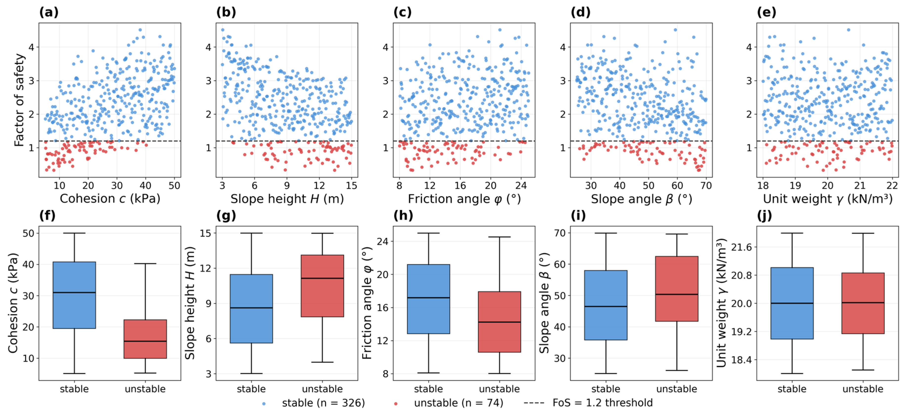
Figure 3 juxtaposes, for each parameter, the scatter of FoS values (Figure 3a–e) and the distributions within the stable and unstable groups (Figure 3f–j).

Cohesion exhibits the clearest divergence. Stable cases span the whole range up to 50 kPa, whereas unstable cases cluster below about 25 kPa, and the separation between the stable and unstable distributions indicates a positive association between c and FoS, consistent with the direct contribution of cohesion to shear resistance. The median cohesion of stable slopes (31.0 kPa) is more than double that of unstable slopes (15.4 kPa), with limited overlap between the interquartile ranges. Cohesion produces by far the strongest separation between the two classes, with the largest KS statistic (D = 0.470, RSI = 38.2%).

Slope height and friction angle show the same pattern with weaker contrast: unstable configurations concentrate at greater heights (median 11.1 m against 8.6 m) and lower friction angles (median 14.2° against 17.2°), as expected since taller slopes generate larger driving moments and lower φ reduces the mobilised resistance. Both yield similar KS statistics (D ≈ 0.26, RSI ≈ 21%), and their partially overlapping distributions indicate that they are significant but individually insufficient predictors of instability.

For slope angle, the overlap is extensive: unstable configurations are somewhat more frequent above ≈50° (median 50.3° against 46.5°), consistent with its lower D value (0.165). For unit weight, the scatter clouds and the boxplots are almost superimposed over the whole 18–22 kN/m³ range (near-identical medians of 20.0 kN/m³ in both classes), anticipating a statistically non-significant sensitivity index (D = 0.075, RSI = 6.1%).

3.2. Cumulative Distribution Functions and KS Statistics

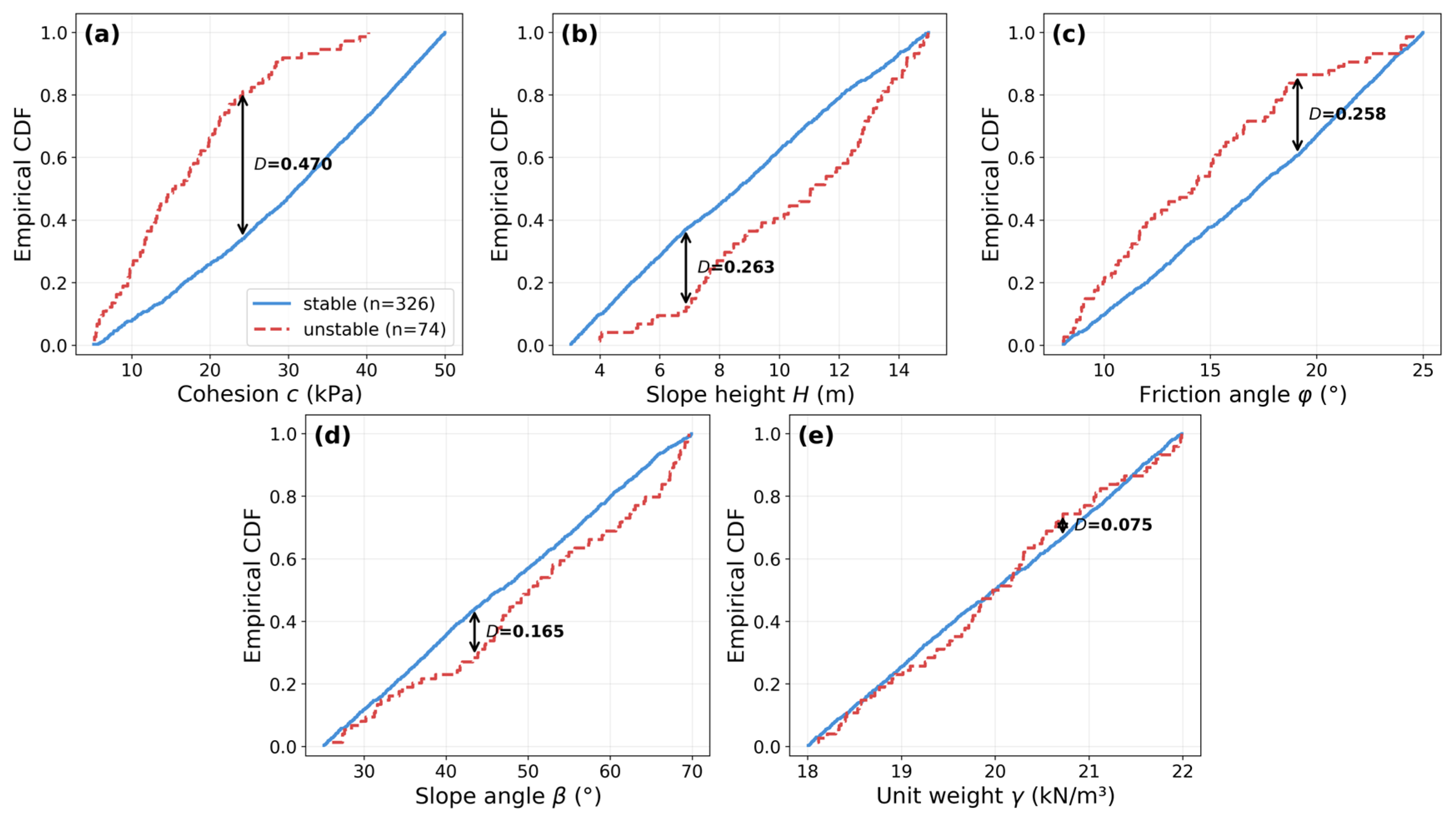
The RSA ranking rests on the empirical CDFs of the stable and unstable populations (Figure 4), the KS statistic D being the maximum vertical distance between them.

The gap for cohesion is pronounced (D = 0.470, p < 0.001): the unstable population is persistently shifted towards lower values, with maximum separation at c ≈ 24 kPa and a divergence above 0.45 over 21–30 kPa, identifying this interval as the critical discrimination zone. The CDFs for height and friction angle diverge in opposite senses—greater heights and lower friction angles promote instability—and both are statistically significant (D = 0.263 and 0.258 respectively, both p < 0.001). For slope angle, the gap (D = 0.165, p = 0.065) falls just short of significance (Dcrit = 0.175): unstable configurations are more frequent at steeper angles, but the trend is not statistically resolvable under the conditions of this study; the reasons are examined in Section 4.1. For unit weight, the two CDFs are almost identical (D = 0.075, p = 0.862), compatible with pure sampling variability.

3.3. Parameter Ranking

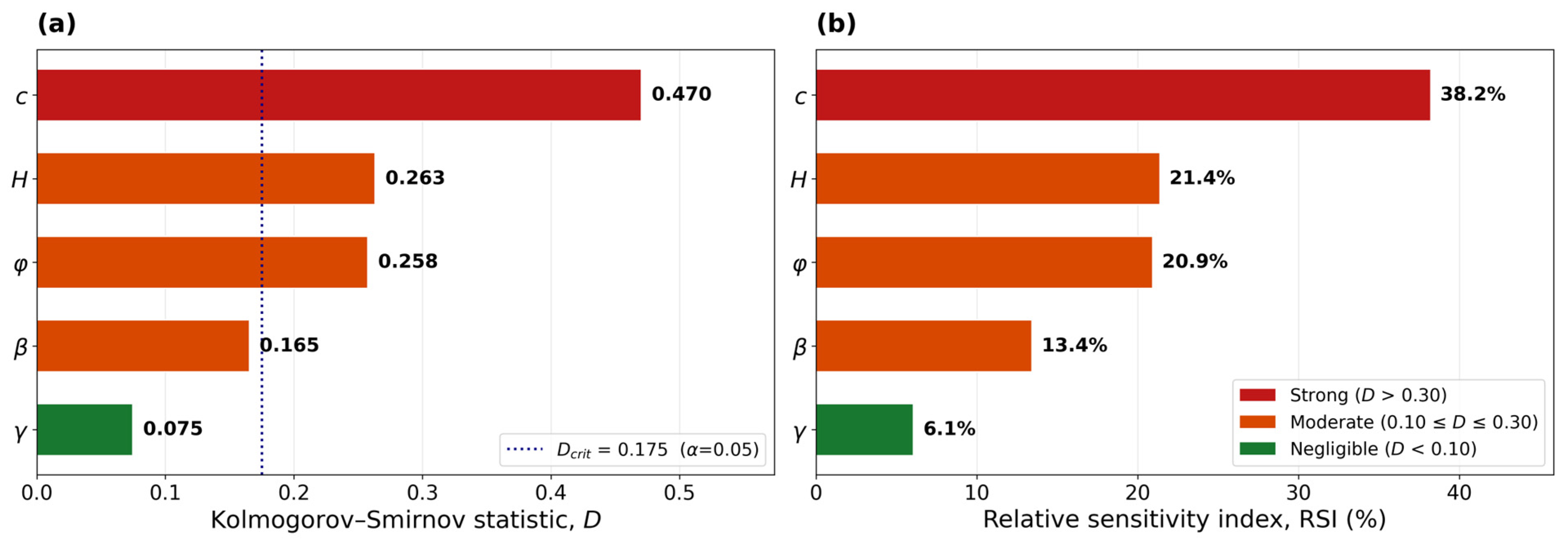
The RSA results are combined into a single ranking in Figure 5 and

Table 2. Regional sensitivity analysis at the reference threshold FoS = 1.2 (ns = 326 stable, nu = 74 unstable; Dcrit = 0.175 at α = 0.05).

Rank	Parameter	D (KS)	RSI (%)	p-Value	Significant
1	Cohesion, c	0.470	38.2	<0.001	yes
2	Height, H	0.263	21.4	<0.001	yes
3	Friction angle, φ	0.258	20.9	<0.001	yes
4	Slope angle, β	0.165	13.4	0.065	no
5	Unit weight, γ	0.075	6.1	0.862	no

.

Three parameters exceed the critical significance threshold Dcrit = 0.175 at α = 0.05: cohesion (D = 0.470), height (D = 0.263) and friction angle (D = 0.258). Slope angle (D = 0.165) and unit weight (D = 0.075) fall below it. Normalising the KS statistics into relative sensitivity indices yields the following hierarchy:

• cohesion c: RSI = 38.2%—strong influence (D > 0.30), dominant parameter;
• slope height H: RSI = 21.4%—moderate influence (0.10 ≤ D ≤ 0.30);
• friction angle φ: RSI = 20.9%—moderate influence (0.10 ≤ D ≤ 0.30);
• slope angle β: RSI = 13.4%—moderate effect size (0.10 ≤ D ≤ 0.30) but not statistically significant at this threshold; borderline;
• unit weight γ: RSI = 6.1%—negligible influence (D < 0.10).

Cohesion, height and friction angle together account for 80.5% of the cumulative RSI. Because RSA measures the divergence induced by each parameter’s assigned variability, this ranking expresses which uncertainties most govern the outcome rather than which parameters exert the largest mechanical effect per unit change; cohesion leads because its plausible in situ variability, driven by the variable degree of weathering, is both wide and consequential.

Bootstrap resampling of the 400 realisations (10,000 resamples) confirms that the fine distinctions are not resolvable at this sample size. The 95% confidence intervals are D(c) = 0.470 [0.41, 0.59], D(H) = 0.263 [0.20, 0.39], D(φ) = 0.258 [0.19, 0.38], D(β) = 0.165 [0.11, 0.30] and D(γ) = 0.075 [0.08, 0.22]. The bootstrap distribution of a two-sample KS statistic is biassed upward, since resampling with replacement introduces ties that inflate the maximum vertical distance; the intervals are therefore shifted above the point estimates. For unit weight the point estimate falls marginally below the lower bound. This does not affect interpretation: the entire interval for γ lies below the critical value at every threshold.

Cohesion’s interval is separated from all others, so its dominance is robust to sampling variability. The interval for D(H) − D(φ) spans zero ([−0.12, +0.14], with H exceeding φ in 56% of resamples): height and friction angle are, in practice, tied. The interval for D(β) straddles the critical value, so its borderline classification is a genuine feature of the data. Cohesion remains significant under a conservative Bonferroni correction for the 20 tests (α = 0.0025) at all four thresholds, as does friction angle (p ≤ 0.002). Slope height remains significant at FoS = 1.1 and 1.2 but falls just above the corrected threshold at FoS = 1.3 and 1.4 (p = 0.003 and 0.004), reflecting the reduced power of the design at stricter thresholds. Unit weight never reaches corrected significance, and neither does slope angle at any threshold—reinforcing the reading of its role as a statistical power effect (Section 3.4).

3.4. Robustness to the Stability Threshold

Table 3. Robustness of the regional sensitivity analysis to the stability threshold. The same 400 simulations are reclassified at each threshold. nu, number of unstable configurations; Dcrit, critical KS value at α = 0.05.

	FoS = 1.1			FoS = 1.2			FoS = 1.3			FoS = 1.4
nu/Dcrit	59/0.192			74/0.175			80/0.170			86/0.166
Parameter	D	RSI (%)	p	D	RSI (%)	p	D	RSI (%)	p	D	RSI (%)	p
Cohesion, c	0.517	36.9	<0.001	0.470	38.2	<0.001	0.456	38.7	<0.001	0.445	38.7	<0.001
Height, H	0.299	21.3	<0.001	0.263	21.4	<0.001	0.222	18.8	0.003	0.210	18.2	0.004
Friction angle, φ	0.292	20.8	<0.001	0.258	20.9	<0.001	0.228	19.4	0.002	0.232	20.2	0.001
Slope angle, β	0.174	12.4	0.083	0.165	13.4	0.065	0.188	15.9	0.020	0.171	14.8	0.034
Unit weight, γ	0.119	8.5	0.438	0.075	6.1	0.862	0.084	7.2	0.734	0.093	8.1	0.561
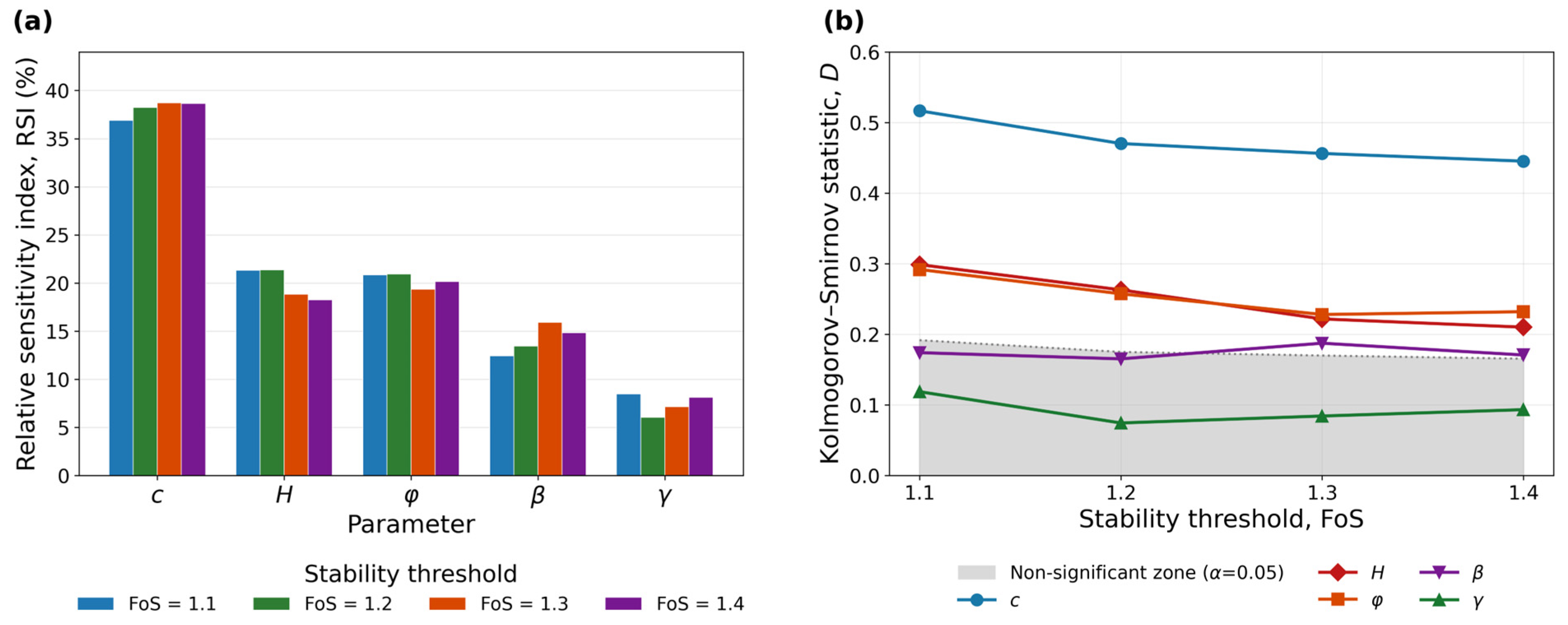
Σ RSI (c, H, φ)	79.1			80.5			76.9			77.1

and Figure 6 report the RSA repeated on the same 400 simulations for FoS thresholds of 1.1, 1.2, 1.3 and 1.4.

The unstable set grows from 59 to 86 configurations, and Dcrit falls accordingly from 0.192 to 0.166. Figure 6a highlights the stability of the hierarchy; Figure 6b the location of each KS statistic relative to the significance boundary.

Three findings are threshold-independent: cohesion ranks first at every threshold (D = 0.445–0.517, RSI = 36.9–38.7%, p < 0.001 throughout); unit weight is never significant (p ≥ 0.438); and c, H and φ together account for 76.9–80.5% of the cumulative RSI. The core result is therefore not an artefact of the threshold chosen.

Two findings are threshold-dependent. D(H) decreases monotonically with the threshold (0.299 → 0.210) while D(φ) decreases more slowly (0.292 → 0.232), so the second and third ranks exchange between FoS = 1.2 and 1.3; since the two statistics differ by less than 0.03 at every threshold, this exchange confirms that H and φ are of comparable influence rather than revealing a physical reordering. Slope angle is more instructive: its KS statistic fluctuates non-monotonically within a narrow band (0.165–0.188) with no systematic trend across thresholds, yet β passes from non-significant at FoS ≤ 1.2 to significant at FoS ≥ 1.3—not because its discriminating power grows, but because the enlargement of the unstable set lowers the critical value from 0.192 to 0.166. The apparent emergence of slope angle as a controlling parameter at stricter thresholds is a statistical power effect, not a mechanical one; reporting its significance from a single threshold would be misleading in either direction.

4. Discussion

4.1. Mechanical Interpretation of the Ranking

The ranking is consistent with limit equilibrium mechanics. Cohesion leads because, over the wide range explored (5–50 kPa), it produces large variations in the resisting term, an effect amplified in marls, whose sensitivity to weathering and moisture makes c the most variable field parameter [3,11]. The secondary roles of H and φ reflect the two sides of the equilibrium balance: taller slopes mobilise larger driving moments, while lower friction angles reduce the resisting shear force mobilised along the failure surface.

The weak ranking of slope angle deserves a careful reading. Steepness matters mechanically, but its effect is strongly conditioned by the values of H and c with which it combines; because the KS statistic is a marginal measure (Section 2.5), such interaction-borne influence is systematically under-represented in the ranking, and the masking by the much larger variability of the shear strength parameters over the space investigated (β ∈ [25°, 70°]) compounds this. The low D of β should be read as “weakly discriminating in isolation”, not as “mechanically unimportant”.

The negligible effect of unit weight stems primarily from the narrowness of its natural range: a 22% span in γ (18–22 kN/m³) cannot generate the FoS contrast that a tenfold span in c generates. A secondary, structural effect reinforces this: γ enters both the driving term and, through the normal force, the frictional resisting term of Equation (3), so that its influence on FoS partially self-compensates—exactly so in the purely frictional case (c = 0), and partially in the cohesive-frictional case studied here.

4.2. Comparison with Previous Studies

The hierarchy c > H ≈ φ > β > γ is broadly consistent with the sensitivity literature, which repeatedly identifies the shear strength parameters as dominant and unit weight as marginal [14,16,17,22]. A recent review similarly singles out cohesion as the critical factor in machine-learning predictions of slope stability [20], and the parametric machine-learning study of Trinidad and Momayez reaches the same hierarchy for rock slopes, with cohesion and friction angle governing the factor of safety and unit weight least influential [21]. Ram et al. [22], analysing local instability between soil nails, likewise found cohesion, friction angle and slope inclination to control the factor of safety; the convergence of results obtained by independent methods is a useful cross-check.

Two differences deserve comment. First, several finite element studies rank the friction angle above cohesion. This is not contradictory: sensitivity rankings are conditional on the ranges assigned to each parameter, and studies exploring a narrow cohesion range with a wide friction range will reverse the order—rankings are not transferable between sites without re-examining those ranges, a point Section 3.4 reinforces for the behavioural threshold. Second, studies of residual soils under rainfall consistently identify the water regime as a first-order control [38]; it is deliberately excluded here and is the subject of the companion study announced in Section 5.

4.3. Implications for Site Investigation

The ranking translates directly into investigation priorities. Effort should go first to characterising cohesion—laboratory testing on intact specimens and in situ measurement, distinguishing peak from residual values in weathered horizons; then to accurate topographic survey (slope height) and determination of the friction angle. Unit weight may be estimated from standard correlations without materially degrading the predicted FoS. Because the CDFs of cohesion separate most strongly over 21–30 kPa, testing should in particular resolve whether the in situ cohesion of a given horizon lies above or below this band. Although calibrated on Moulay Yacoub, the ranking is expected to transfer to other weathered argillaceous formations whose strength is governed by the degree of weathering—peri-Mediterranean Neogene marls, clay-shales and comparable soft rocks—because the mechanism driving cohesion’s dominance (a wide, weathering-controlled range of c against a narrow range of γ) is shared across these materials. The transfer is conditional: it holds where the cohesion range is comparably wide (Section 3.4). What generalises is the procedure—characterise cohesion first, and resolve whether the in situ value falls within the locally identified discrimination band—rather than the specific 21–30 kPa band, which is site-dependent.

4.4. Limitations

Six limitations restrict the interpretation of these results. First, the five parameters were sampled independently from uniform marginal distributions. In weathered marls, both cohesion and the friction angle vary together with the extent of weathering; consequently, independent sampling can produce mechanically implausible pairings—e.g., c > 40 kPa paired with φ < 14° (7.5% of the design). The design is appropriate for a screening exercise—ranking inputs over their plausible ranges—but not for reliability analysis, and the coefficients of variation in geotechnical parameters differ substantially in reality [39]. The proportion of unstable realisations (18.5% at FoS = 1.2) is thus a property of the sampling, not a probability of failure.

Second, the ranking is conditional on the ranges of Table 1: the KS statistic of cohesion in particular reflects the width of its assigned range as much as its mechanical role. This dependence was tested directly. Truncating the design to c ≤ 30 kPa lowers D(c) from 0.470 to 0.216 and exchanges the first two ranks, height then leading (D(H) = 0.263, essentially unchanged); truncating to c ≤ 25 kPa renders cohesion non-significant. This is expected rather than contradictory: removing the high-cohesion configurations discards precisely the region where cohesion best separates the two classes—only six of the 74 unstable configurations have c > 30 kPa—and the reduced sample raises the critical value from 0.175 to 0.198. The dominance of cohesion is therefore an uncertainty-governance statement—cohesion is the parameter whose plausible variability, driven by the variable degree of weathering, most governs the computed stability—rather than a claim of maximal mechanical influence per unit change.

Third, pore water pressure is neglected. Of the two mechanisms by which water destabilises marly slopes, the softening of the weathered mantle is partially internalised here—the lower portion of the 5–50 kPa cohesion range represents moisture-affected, softened states—whereas the direct effective-stress effect of pore pressure is excluded. The ranking therefore applies to the drained, deep-water-table configuration, and the strong sensitivity to cohesion should be expected to persist, or intensify, under wetting, since infiltration drives the marl towards the low-cohesion region where the two populations separate most strongly. Seasonal infiltration and leakage from urban networks are documented destabilising factors at Moulay Yacoub [4]; the companion study announced in Section 5 addresses the pore-pressure mechanism explicitly.

Fourth, the slope was modelled as a single homogeneous layer; stratification, fissuring and the strength contrast between weathered and unweathered marl, reported in comparable formations [11], are not represented.

Fifth, the crest surcharge was held constant at 20 kN/m² rather than sampled. Its plausible range at the site (10–30 kN/m²) is not negligible, and the ranking therefore quantifies the governance of the soil and geometric uncertainties conditional on a fixed exposure level. A design in which the surcharge were sampled could plausibly place it among the significant inputs; this is a limitation of scope rather than a claim of insensitivity.

Sixth, failure surfaces were assumed circular. For the steepest configurations, critical mechanisms are frequently non-circular or controlled by tension cracks, and this regime is populated in the design: 31% of the unstable realisations at FoS = 1.2 have β > 60°, against 22% of the full design. The factor of safety of these configurations may therefore be overestimated relative to a non-circular analysis. In addition, the factor of safety is obtained as the minimum over a discrete search of circular surfaces; for realisations close to the stability threshold this introduces an uncertainty of the order of ±0.1–0.2 in the computed value, and hence some ambiguity in the binary classification. The threshold-robustness analysis and the bootstrap confidence intervals together show that the parameter ranking is insensitive to this classification uncertainty.

The circular search was, moreover, constrained to pass through a fixed base point at the toe of the sampled slope—the junction with the lower slope segment, whose geometry is fixed across all 400 configurations—so that circles daylighting on the slope face above this toe were not part of the primary search. Because the critical circle of a steep slope is theoretically a toe circle [40], such face mechanisms are not expected to govern; this was verified directly. The behavioural configurations near the reference threshold most susceptible to a shallow mechanism—those combining low cohesion with a steep face—together with the steepest, lowest-cohesion unstable cases, were recomputed with the search forced onto an intermediate horizon within the weathered mantle, so that circles daylighted on the face. In every case the face-daylighting surface was markedly less critical than the toe circle: for the near-threshold behavioural configurations the minimum factor of safety rose to approximately 2.0 (from 1.21 to 1.28), and none crossed the FoS = 1.2 threshold. A complementary check on configurations spanning the design extremes, with the search relaxed toward deeper surfaces tangent to a fixed horizon below the toe, likewise left every classification at FoS = 1.2 unchanged. The toe-reaching circle is therefore confirmed as the governing surface, and the parameter ranking is insensitive to the search constraint.

5. Conclusions

This work ranked the parameters governing the computed stability of weathered marl slopes at Moulay Yacoub, from 400 Latin-hypercube configurations over site-derived ranges, factors of safety computed with Bishop’s simplified method in Talren, and regional sensitivity analysis based on the Kolmogorov–Smirnov statistic and a relative sensitivity index.

Over the ranges investigated and under dry conditions, the hierarchy of uncertainty governance is c > H ≈ φ > β > γ. Cohesion is the parameter whose plausible variability most governs the computed stability, accounting for close to 38% of the cumulative sensitivity; slope height and friction angle contribute about 20% each and are statistically indistinguishable; slope angle is borderline; unit weight is not discriminating. Beyond the ranking itself, the analysis yields a site-specific, actionable product: the 21–30 kPa cohesion band over which the stable and unstable populations separate most strongly, and which testing at comparable sites should aim to resolve.

Repeating the analysis at four stability thresholds establishes which of these statements survive the modelling choice. The dominance of cohesion and the irrelevance of unit weight hold at every threshold between 1.1 and 1.4; the ordering of slope height and friction angle does not; and the apparent significance of the slope angle at stricter thresholds is a consequence of the enlarged unstable set, not of increased discriminating power. Threshold sensitivity thus determines which conclusions may legitimately be drawn from a regional sensitivity analysis.

A companion study incorporating a variable phreatic surface into the same parametric framework is under way; water table depth is expected to emerge as a controlling factor alongside cohesion and slope height.

References

1. Froude, M.J.; Petley, D.N. Global Fatal Landslide Occurrence from 2004 to 2016. Nat. Hazards Earth Syst. Sci. 2018, 18, 2161–2181. [Google Scholar] [CrossRef] [Scilit]
2. Picarelli, L.; Urciuoli, G.; Ramondini, M.; Comegna, L. Main Features of Mudslides in Tectonised Highly Fissured Clay Shales. Landslides 2005, 2, 15–30. [Google Scholar] [CrossRef] [Scilit]
3. Vaughan, P.R.; Leroueil, S. Discussion: The General and Congruent Effects of Structure in Natural Soils and Weak Rocks. Geotechnique 1991, 40, 281–284. [Google Scholar] [CrossRef] [Scilit]
4. Obda, I.; El Kharim, Y.; Bounab, A.; Lahrach, A.; Ahniche, M.; Mansouri, H. Multi-Criteria Assessment Approach of Slow-Moving Urban Landslide Hazard: The Case of Moulay Yacoub, Morocco. Can. J. Earth Sci. 2021, 59, 300–317. [Google Scholar] [CrossRef] [Scilit]
5. Obda, I.; Obda, O.; Sahrane, R.; El Kharim, Y.; Lahrach, A.; Ahniche, M. Landslide Susceptibility Mapping Using GIS Matrix Method and Frequency Ratio, Application in the Marly Context of Moulay Yacoub Region, Morocco. Bull. Soc. Géol. Fr. 2024, 195, 1. [Google Scholar] [CrossRef] [Scilit]
6. Medrari, A.; Benzougagh, B.; Ouchen, I.; Tayyeh, H.K.; Hussein, A.M.; Mastere, M.; Benyounes, T.; El Ghazi, N.; Khedher, K.M. Geotechnical Characterization, Risk Analysis, and Design of Stabilization Measures for a Landslide Along the RN16 Coastal Highway in Morocco: A Case Study at KP 178+000. GeoHazards 2026, 7, 68. [Google Scholar] [CrossRef] [Scilit]
7. Akhdar, A.L.; Tarmouchant, A.N.; Ahire, M.D.; Slimane, A.B. Nouvelle Approche Geologique et Geodinamique du Complexe Hydrothermal de Moulay Yacoub (Bordure Septentrionale du Sillon Sud Rifain). Comun. Geol. 2006, 93, 185–204. [Google Scholar]
8. El Amrani Paaza, N.; Lamas, F.; Irigaray, C.; Chacón, J. Engineering Geological Characterization of Neogene Marls in the Southeastern Granada Basin, Spain. Eng. Geol. 1998, 50, 165–175. [Google Scholar] [CrossRef] [Scilit]
9. Alonso, E.E.; Pineda, J.A.; Cardoso, R. Degradation of Marls; Two Case Studies from the Iberian Peninsula. Geol. Soc. Lond. Eng. Geol. Spec. Publ. 2010, 23, 47–75. [Google Scholar] [CrossRef] [Scilit]
10. Lamas, F.; Oteo, C.; Chacón, J. Influence of Carbonate Content on the Stress–Strength Behaviour of Neogene Marls from the Betic Cordillera (Spain) in Cu Triaxial Tests Using a Quasilinear Elastic (Hyperbolic) Model. Eng. Geol. 2011, 122, 160–168. [Google Scholar] [CrossRef] [Scilit]
11. Alonso, E.E.; Pinyol, N.M. Slope Stability in Slightly Fissured Claystones and Marls. Landslides 2015, 12, 643–656. [Google Scholar] [CrossRef] [Scilit]
12. Duncan, J.M. State of the Art: Limit Equilibrium and Finite-Element Analysis of Slopes. J. Geotech. Eng. 1996, 122, 577–596. [Google Scholar] [CrossRef] [Scilit]
13. Hammah, R.; Yacoub, T.; Corkum, B.; Curran, J. A Comparison of Finite Element Slope Stability Analysis with Conventional Limit-Equilibrium Investigation. In Proceedings of the Proceedings of the 58th Canadian Geotechnical and 6th Joint IAH-CNC and CGS Groundwater Specialty Conferences (GeoSask 2005), Saskatoon, Canada, 18–21 September 2005; pp. 480–487. [Google Scholar]
14. Pianosi, F.; Beven, K.; Freer, J.; Hall, J.W.; Rougier, J.; Stephenson, D.B.; Wagener, T. Sensitivity Analysis of Environmental Models: A Systematic Review with Practical Workflow. Environ. Model. Softw. 2016, 79, 214–232. [Google Scholar] [CrossRef] [Scilit]
15. Agam, M.W.; Hashim, M.H.M.; Murad, M.I.; Zabidi, H. Slope Sensitivity Analysis Using Spencer’s Method in Comparison with General Limit Equilibrium Method. Procedia Chem. 2016, 19, 651–658. [Google Scholar] [CrossRef] [Scilit]
16. Ning, Y.; Tang, H.; Wang, F.; Zhang, G. Sensitivity Analysis of Toppling Deformation for Interbedded Anti-Inclined Rock Slopes Based on the Grey Relation Method. Bull. Eng. Geol. Environ. 2019, 78, 6017–6032. [Google Scholar] [CrossRef] [Scilit]
17. Wines, D. Understanding the Sensitivity of Numerical Slope Stability Analyses to Geotechnical and Other Input Parameters. In Proceedings of the 2020 International Symposium on Slope Stability in Open Pit Mining and Civil Engineering, Australian Centre for Geomechanics, Perth, Australia, 12–14 May 2020; pp. 983–1002. [Google Scholar]
18. Shirol, S.S.; Chavda, J.T. Sensitivity Analysis of Stability of Rockmass Slope Using Finite Element Limit Analysis. In Proceedings of the Indian Geotechnical Conference 2022 Volume 5; Jose, B.T., Sahoo, D.K., Oommen, T., Muthukkumaran, K., Chandrakaran, S., Santhosh Kumar, T.G., Eds.; Lecture Notes in Civil Engineering; Springer Nature: Singapore, 2024; Volume 483, pp. 53–62. ISBN 978-981-97-3388-0. [Google Scholar]
19. Jing, Y. Factor of Safety Prediction for Slope Stability Using PCA and BPNN in Guangdong’s H Mining Area. Sci. Rep. 2025, 15, 12804. [Google Scholar] [CrossRef] [Scilit] [PubMed]
20. Trinidad, M.; Momayez, M. Machine Learning in Slope Stability: A Review with Implications for Landslide Hazard Assessment. GeoHazards 2025, 6, 67. [Google Scholar] [CrossRef] [Scilit]
21. Trinidad, M.; Momayez, M. Application of Machine Learning Methods for Predicting the Factor of Safety in Rock Slopes. Geotechnics 2026, 6, 15. [Google Scholar] [CrossRef] [Scilit]
22. Ram, B.K.; Koy, C.; Yune, C.-Y. Factor of Safety for the Local Instability of Wedge-Shaped Double Body Failure between Soil Nails. Int. J. Geotech. Eng. 2025, 19, 158–171. [Google Scholar] [CrossRef] [Scilit]
23. Hamm, N.A.S.; Hall, J.W.; Anderson, M.G. Variance-Based Sensitivity Analysis of the Probability of Hydrologically Induced Slope Instability. Comput. Geosci. 2006, 32, 803–817. [Google Scholar] [CrossRef] [Scilit]
24. Rohmer, J.; Foerster, E. Global Sensitivity Analysis of Large-Scale Numerical Landslide Models Based on Gaussian-Process Meta-Modeling. Comput. Geosci. 2011, 37, 917–927. [Google Scholar] [CrossRef] [Scilit]
25. Bravo-Zapata, M.F.; Muñoz, E.; Lapeña-Mañero, P.; Montenegro-Cooper, J.M.; King, R.W. Analysis of the Influence of Geomechanical Parameters and Geometry on Slope Stability in Granitic Residual Soils. Appl. Sci. 2022, 12, 5574. [Google Scholar] [CrossRef] [Scilit]
26. Idris, M.A. Probabilistic Slope Stability Assessment of Laterite Borrow Pit Using Artificial Neural Network. Int. J. Geotech. Eng. 2022, 16, 1152–1164. [Google Scholar] [CrossRef] [Scilit]
27. Savvides, A.-A.; Papadopoulos, L. A Neural Network Model for Estimation of Failure Stresses and Strains in Cohesive Soils. Geotechnics 2022, 2, 1084–1108. [Google Scholar] [CrossRef] [Scilit]
28. Ahmad, H.; Yinghua, Z.; Alam, M.; Khan, M.; Junaid Haider, N.S. An Efficient Reliability Assessment of Coupled FDM-DEM Slope Stability Using Physics-Informed Feature-Based Surrogate Machine Learning Techniques. Comput. Geotech. 2026, 196, 108185. [Google Scholar] [CrossRef] [Scilit]
29. Wang, Y.; Wang, L.; Liu, S.; Han, L.; Zhang, W.; Hong, L.; Zhu, Z.; Zhu, X. Region Similarity Assessment for Empowering Physics-Informed Transfer Learning-Based Landslide Susceptibility Mapping. J. Rock Mech. Geotech. Eng. 2025, in press. [Google Scholar] [CrossRef] [Scilit]
30. Wang, Y.; Zhang, W.; Wang, L.; Liu, S.; Zhang, K.; Liu, P.; Sun, W.; Jiang, S. Cross-Regional Extrapolation of Landslide Susceptibility Mapping via Transfer Learning. Geosci. Front. 2026, 17, 102212. [Google Scholar] [CrossRef] [Scilit]
31. Fredlund, D.G.; Krahn, J. Comparison of Slope Stability Methods of Analysis. Can. Geotech. J. 1977, 14, 429–439. [Google Scholar] [CrossRef] [Scilit]
32. Coop, M.R.; Atkinson, J.H. The Mechanics of Cemented Carbonate Sands. Geotechnique 1993, 43, 53–67. [Google Scholar] [CrossRef] [Scilit]
33. Hungr, O. An Extension of Bishop’s Simplified Method of Slope Stability Analysis to Three Dimensions. Géotechnique 1987, 37, 113–117. [Google Scholar] [CrossRef] [Scilit]
34. Huber, B.; Philipponnat, B.; Payant, O.; Zerhouni, M. Fondations et Ouvrages En Terre: Manuel Professionnel de Géotechnique Du BTP; Eyrolles: Paris, France, 2019. [Google Scholar]
35. McKay, M.D.; Beckman, R.J.; Conover, W.J. Comparison of Three Methods for Selecting Values of Input Variables in the Analysis of Output from a Computer Code. Technometrics 1979, 21, 239–245. [Google Scholar] [CrossRef] [Scilit]
36. Helton, J.C.; Davis, F.J. Latin Hypercube Sampling and the Propagation of Uncertainty in Analyses of Complex Systems. Reliab. Eng. Syst. Saf. 2003, 81, 23–69. [Google Scholar] [CrossRef] [Scilit]
37. Sobol’, I.M. Global Sensitivity Indices for Nonlinear Mathematical Models and Their Monte Carlo Estimates. Math. Comput. Simul. 2001, 55, 271–280. [Google Scholar] [CrossRef] [Scilit]
38. Satyanaga, A.; Aventian, G.D.; Rahardjo, H.; Huang, W.; Hutama, D.A. Experimental and Numerical Approaches for Assessing the Stability Analyses of Shallow Residual Soil Slopes. Int. J. Geotech. Eng. 2025, 19, 382–399. [Google Scholar] [CrossRef] [Scilit]
39. Phoon, K.-K.; Kulhawy, F.H. Characterization of Geotechnical Variability. Can. Geotech. J. 1999, 36, 612–624. [Google Scholar] [CrossRef]
40. Taylor, D.W. Stability of Earth Slopes. J. Boston Soc. Civ. Eng. 1937, 24, 197–246. [Google Scholar]
Figure 1. Field evidence of slope instability at Moulay Yacoub: (a) example of a landslide affecting weathered marls in a zone of Moulay Yacoub, with building immediately behind the slope; (b) unsupported vertical excavation cut into the weathered marl at the slope toe; (c) open ground fractures and escarpments at the foot of the buildings. Source: LPEE/field survey.
Geohazards 07 00099 g001
Figure 2. Simplified theoretical cross-section of the slope model implemented in Talren), showing the weathered marl sliding layer over the unweathered substratum, the slope height H, the slope angle β and the distributed crest surcharge representing the adjacent buildings. The section is schematic and does not represent a surveyed profile of a specific hillslope.
Geohazards 07 00099 g002
Figure 3. Stable–unstable stratification at FoS = 1.2. (ae) Factor of safety against each parameter; blue markers denote stable configurations (n = 326), red markers unstable ones (n = 74); the dashed line marks the FoS = 1.2 threshold. (fj) Distribution of each parameter by stability class, same colour coding. Panels ordered by decreasing KS statistic D.
Geohazards 07 00099 g003
Figure 4. Empirical cumulative distribution functions of each parameter at FoS = 1.2, computed separately for the stable (blue, solid) and unstable (red, dashed) populations: (a) cohesion c; (b) slope height H; (c) friction angle φ; (d) slope angle β; (e) unit weight γ. In each panel, the double arrow marks the Kolmogorov–Smirnov statistic D, the maximum vertical distance between the two curves; the larger this distance, the more strongly the parameter discriminates between the two classes.
Geohazards 07 00099 g004
Figure 5. Regional sensitivity analysis ranking at FoS = 1.2. (a) Kolmogorov–Smirnov statistic D for each parameter, with the critical value Dcrit = 0.175 at α = 0.05 shown as a dotted line; (b) the same ranking expressed as a relative sensitivity index. Bar colours denote the effect-size class: strong (D > 0.30), moderate (0.10 ≤ D ≤ 0.30) and negligible (D < 0.10).
Geohazards 07 00099 g005
Figure 6. Robustness of the ranking to the stability threshold. (a) Relative sensitivity index of each parameter at FoS = 1.1, 1.2, 1.3 and 1.4; (b) Kolmogorov–Smirnov statistic against threshold, with the non-significant zone (D < Dcrit at α = 0.05) shaded.
Geohazards 07 00099 g006