
Tire Wear Reduction Based on an Extended Multibody Rear Axle Model


Abstract
1. Introduction
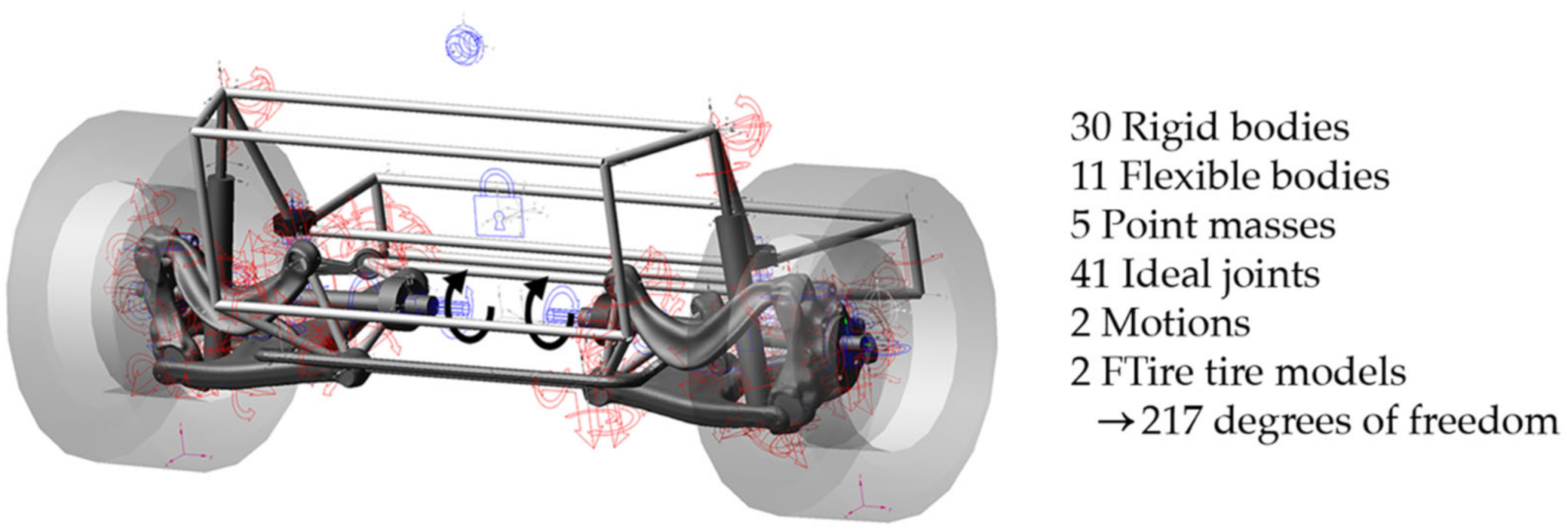
2. Rear Axle Model
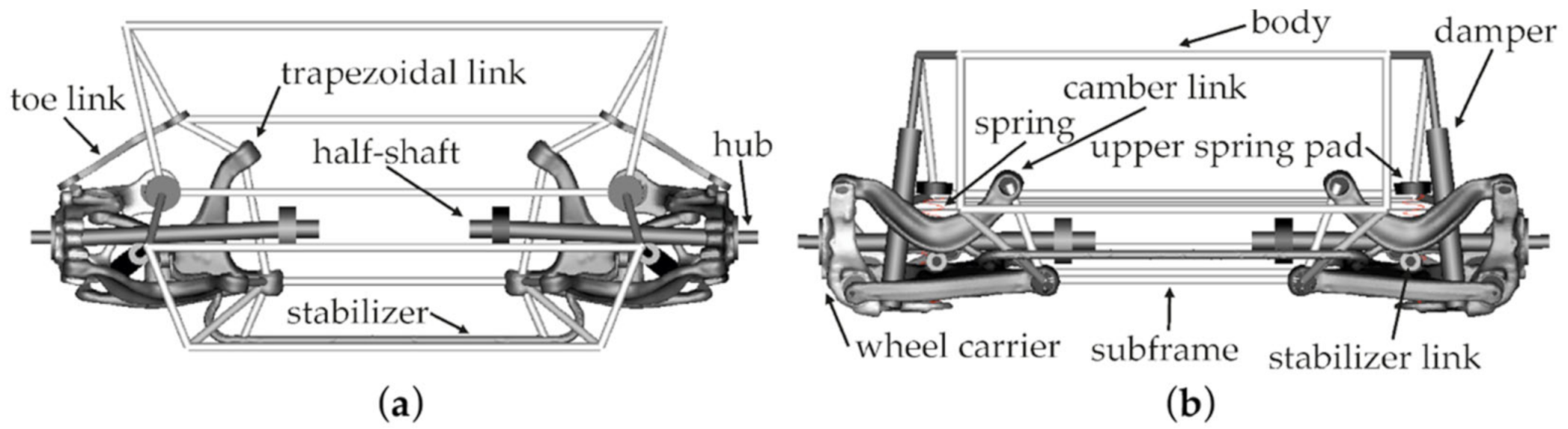
2.1. Kinematic Model
2.2. Elasto-Kinematic Model
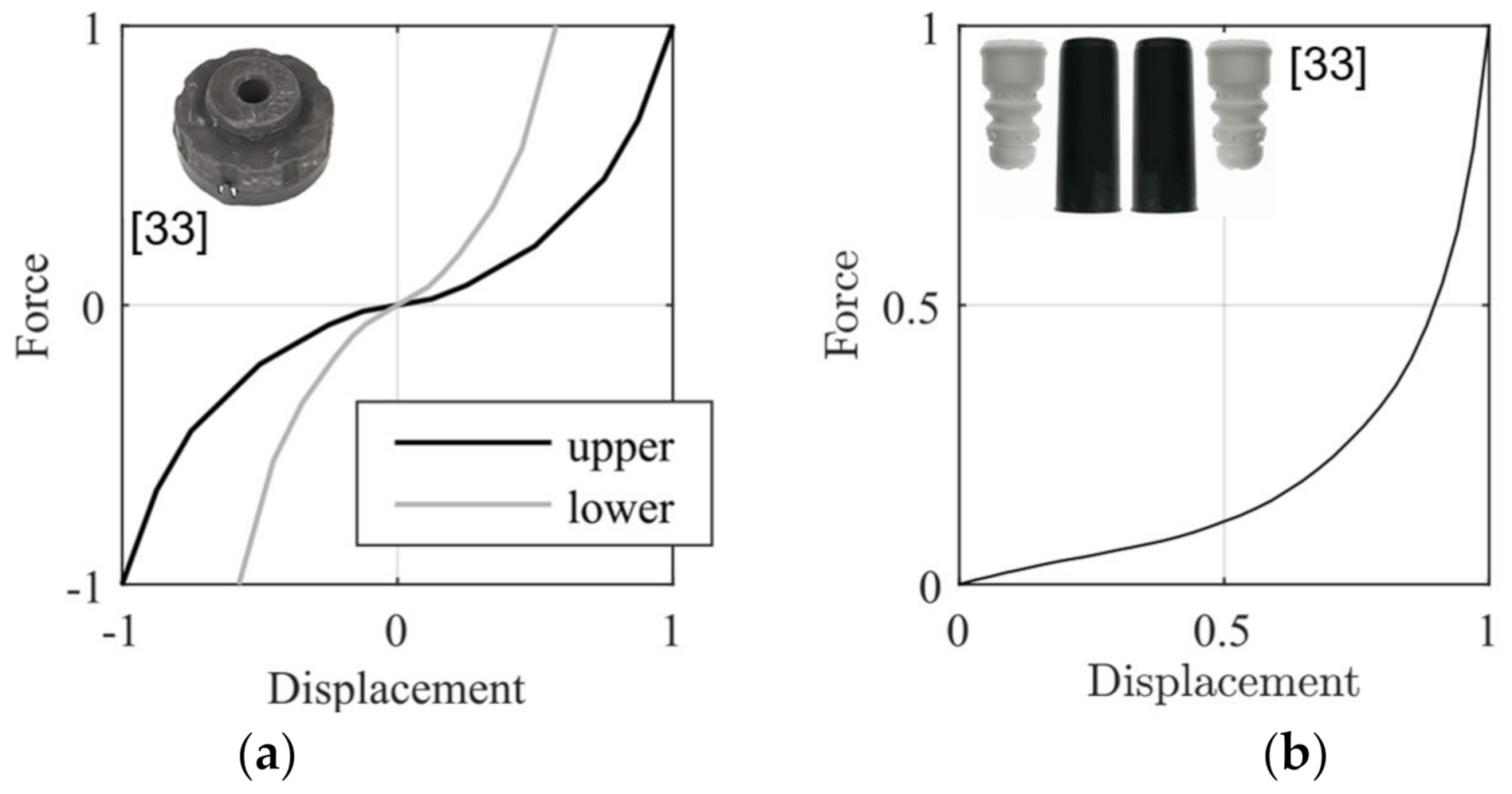
2.2.1. Spring System
2.2.2. Half-Shafts
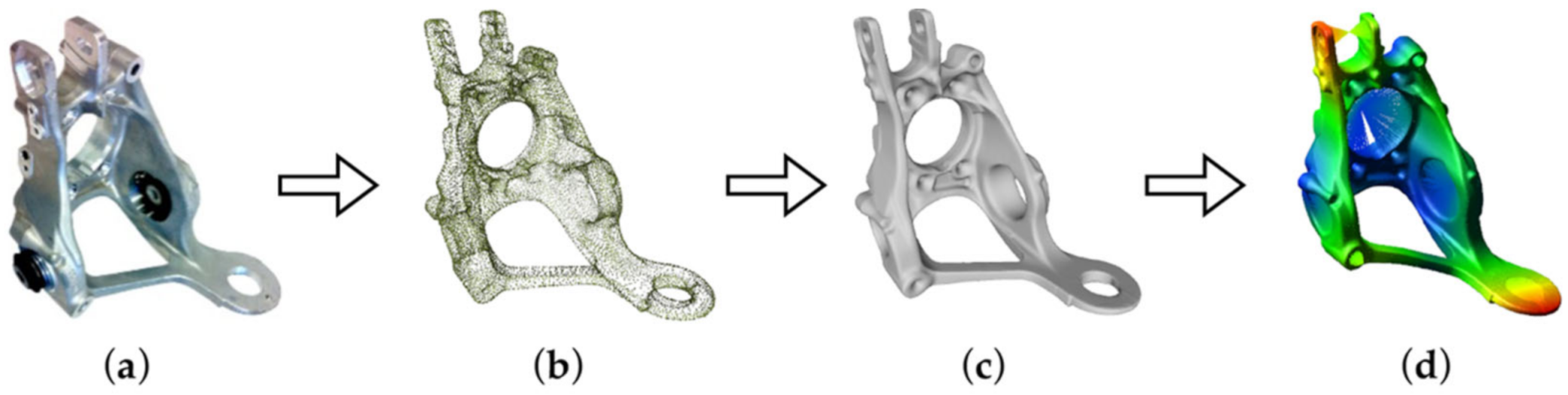
2.2.3. Flexible Bodies
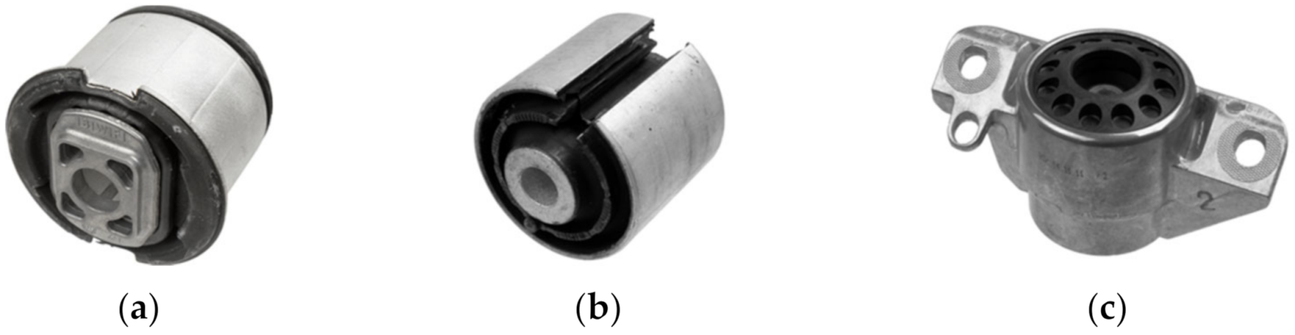
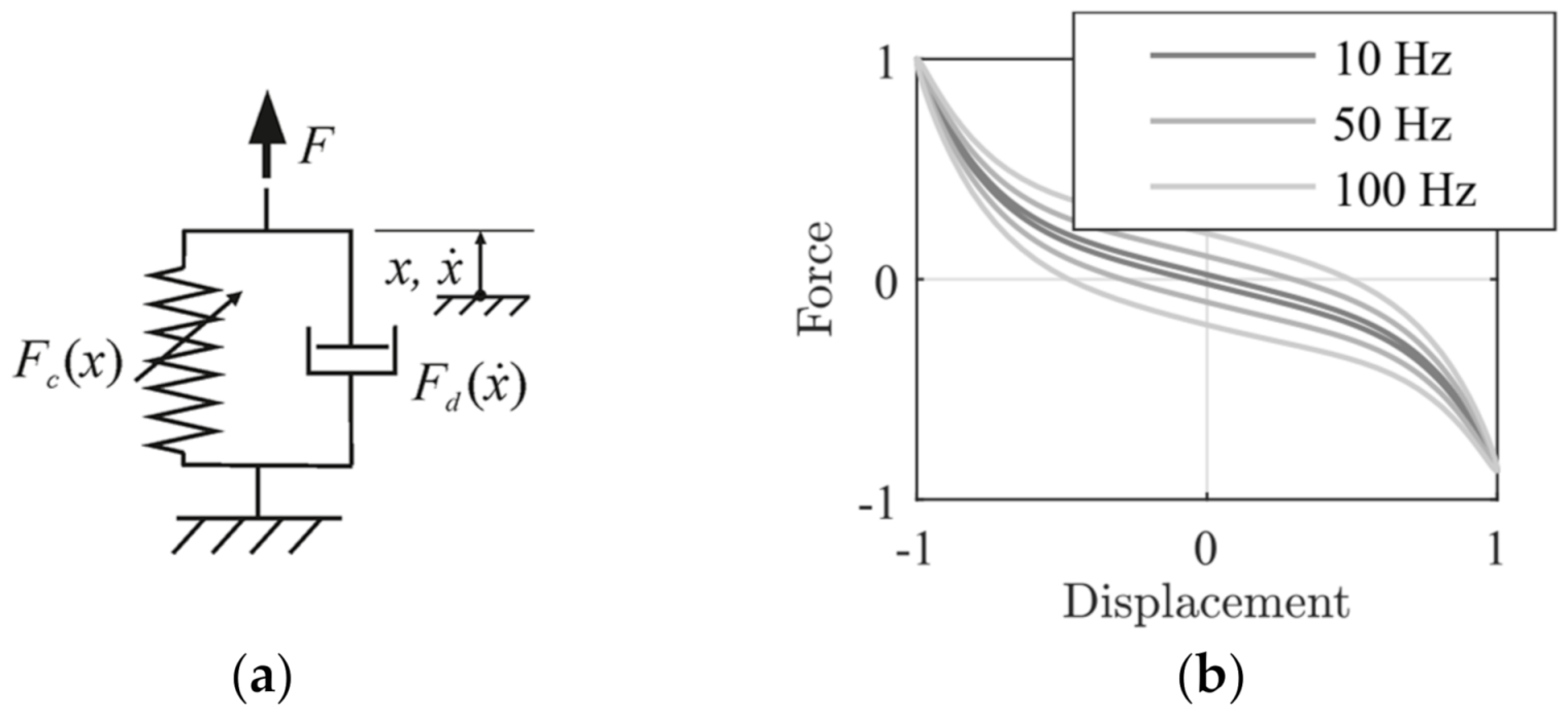
2.2.4. Bushings
2.2.5. Mass and Inertia Distribution
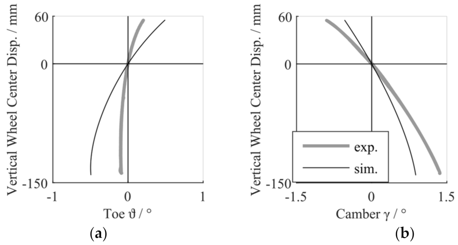
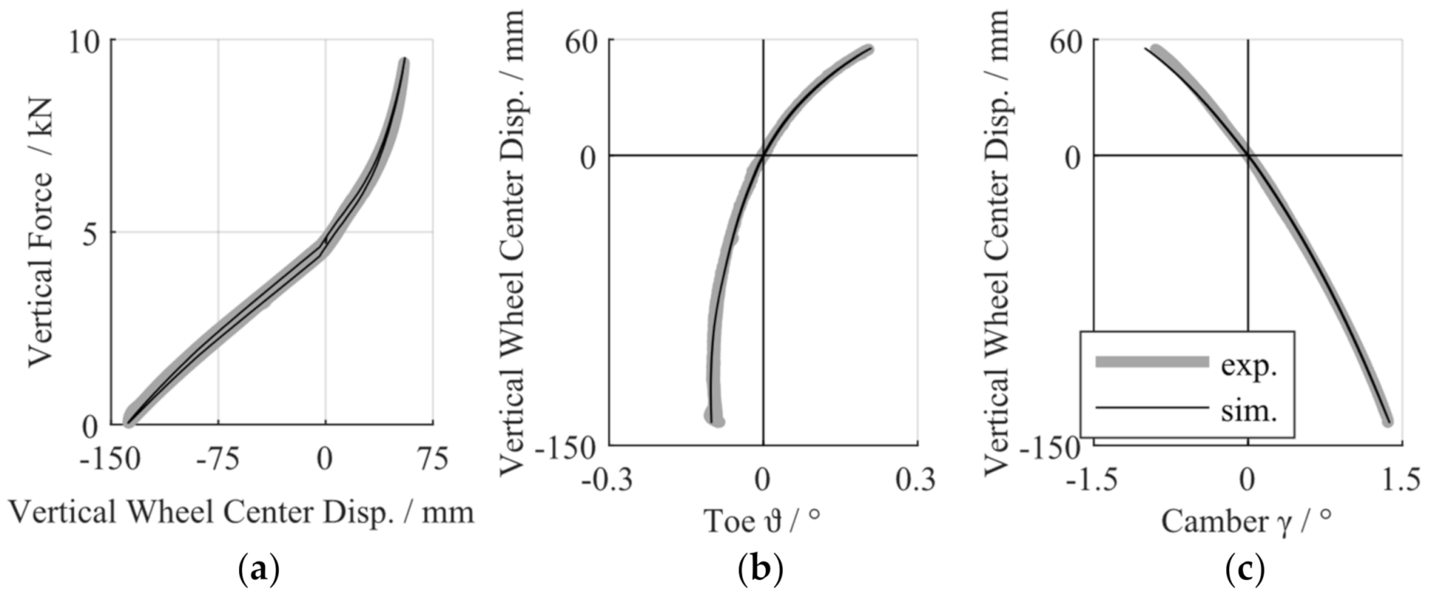
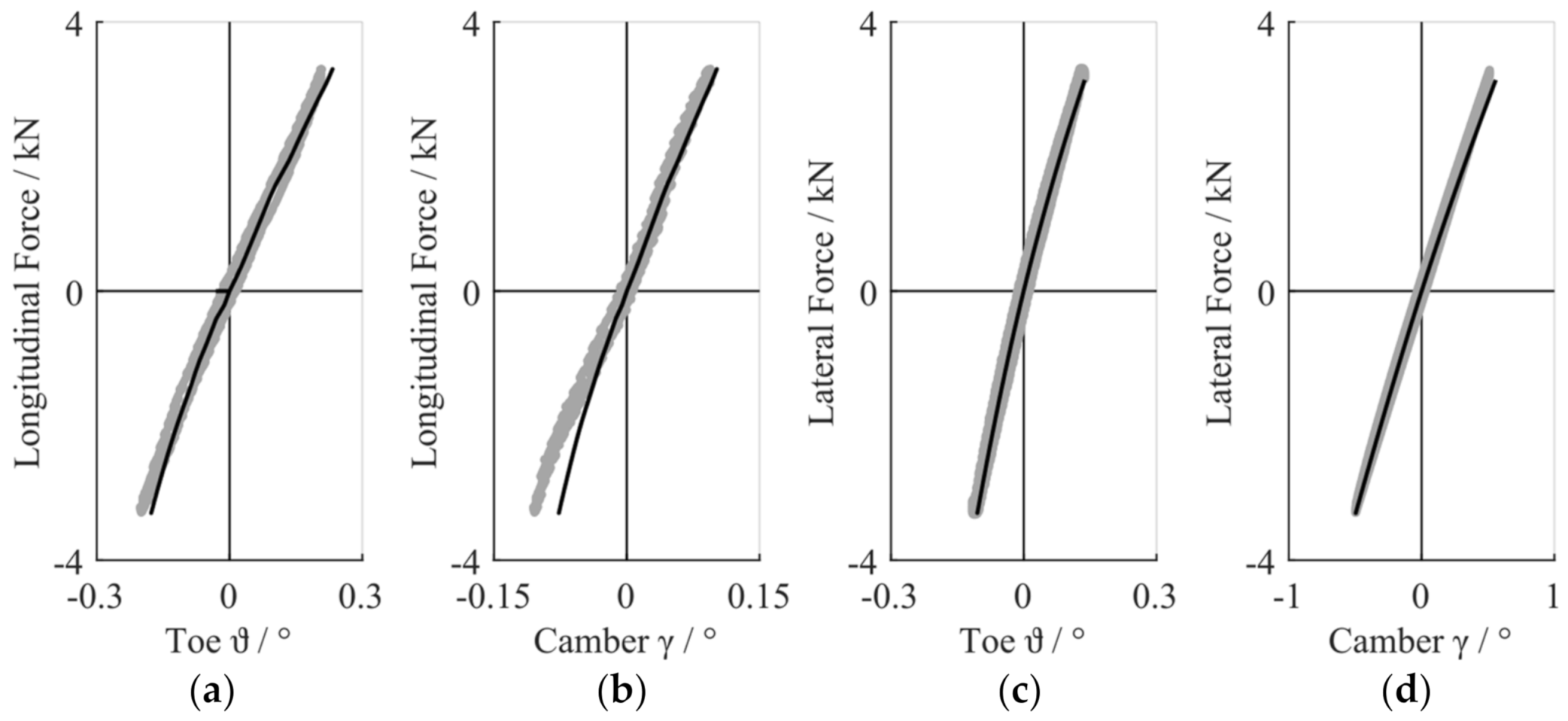
2.2.6. Validation of Elasto-Kinematics
3. Tire and Road Model
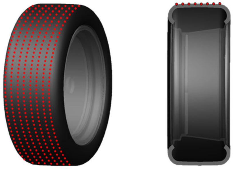
3.1. FTire Tire Model
3.2. Road Model
4. Tire Wear
4.1. Linear Wear Law
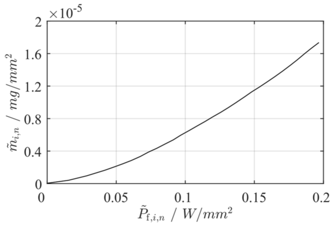
4.2. Nonlinear Wear Law
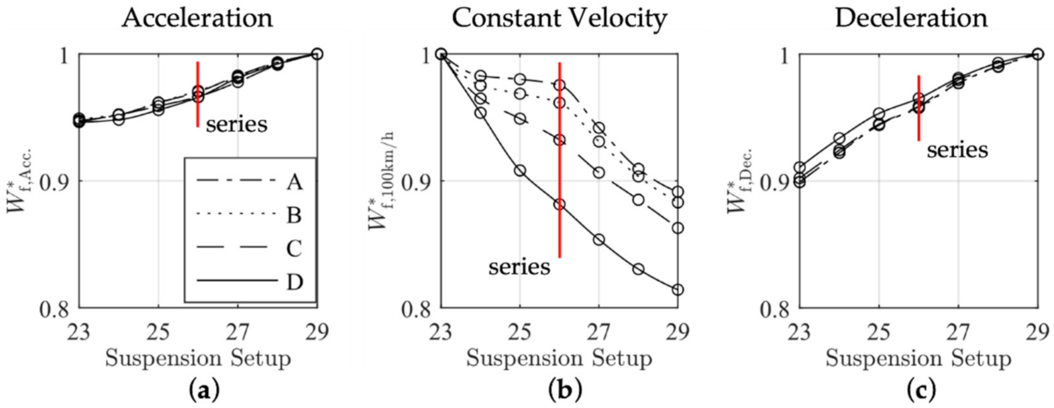
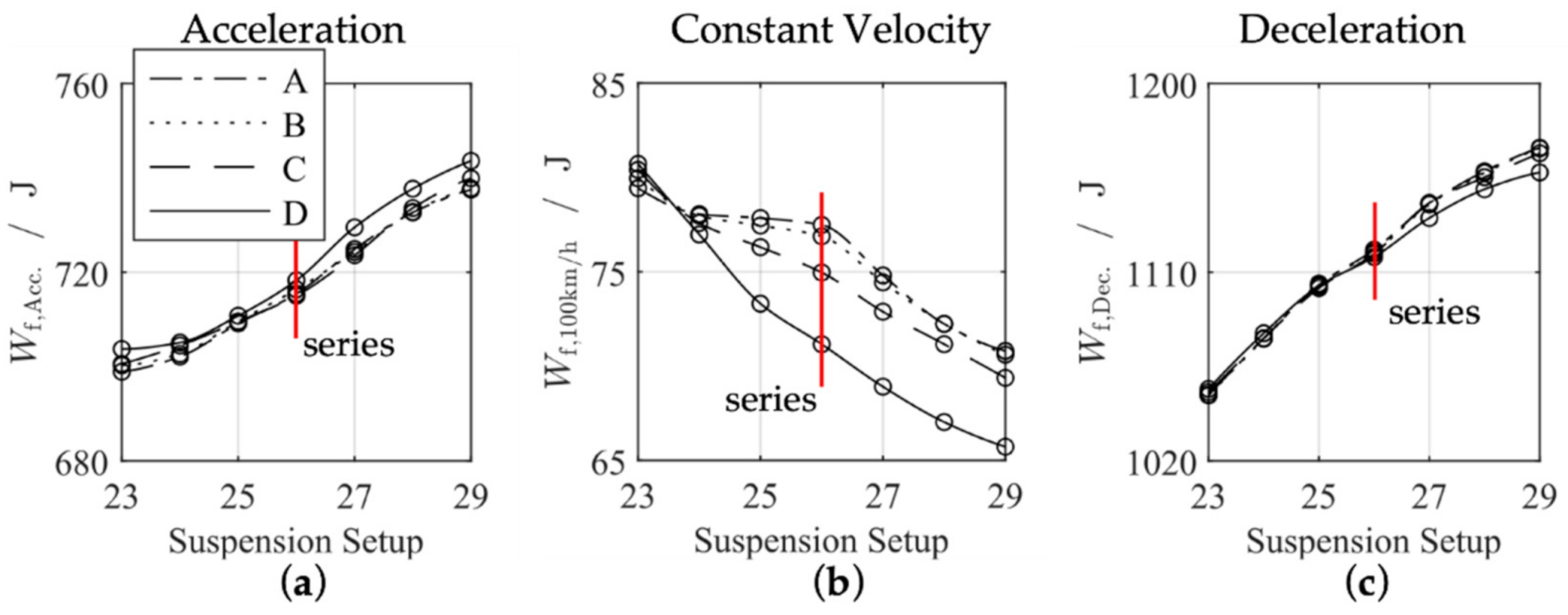
5. Simulation and Results
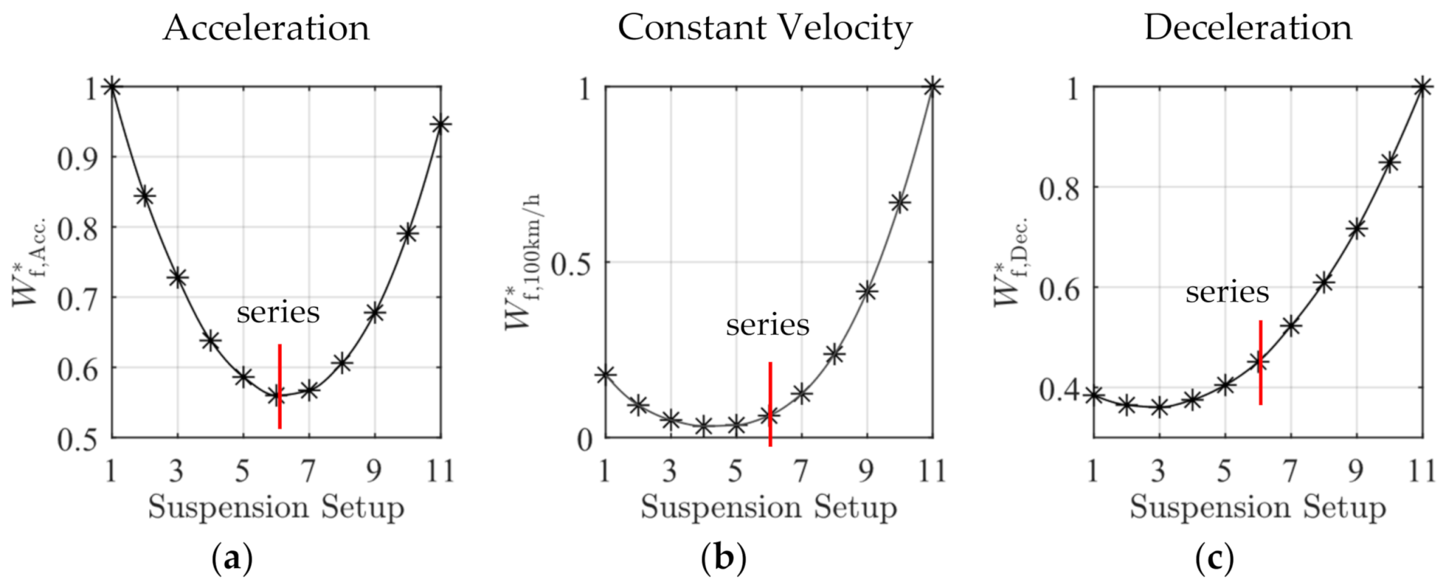
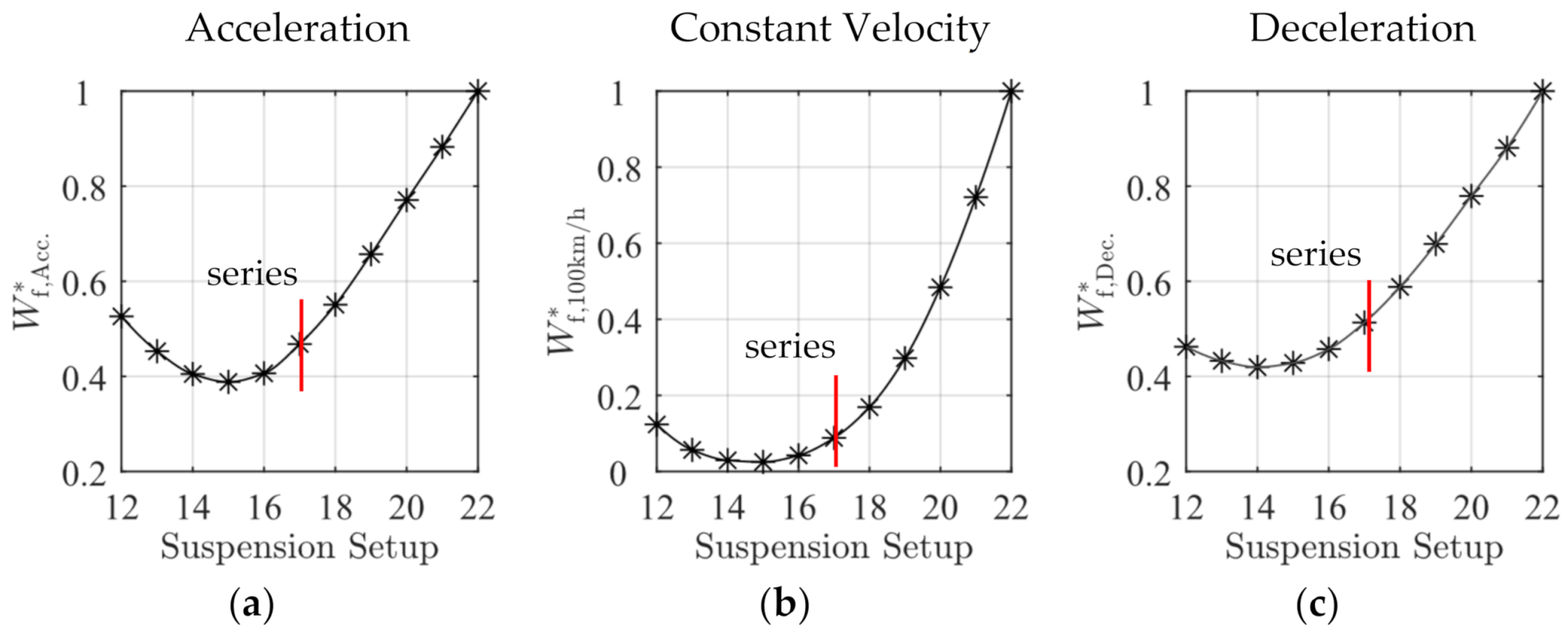
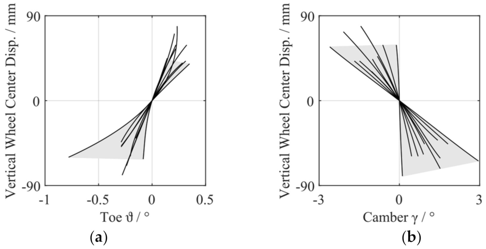
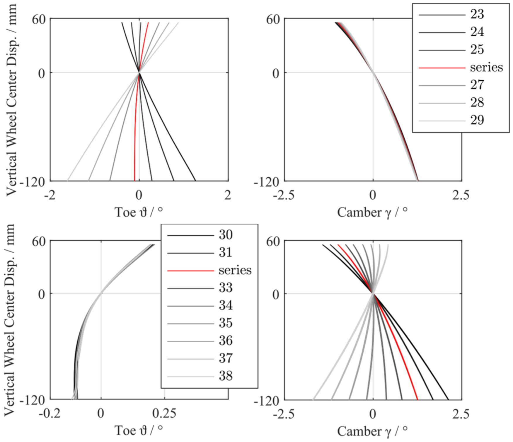
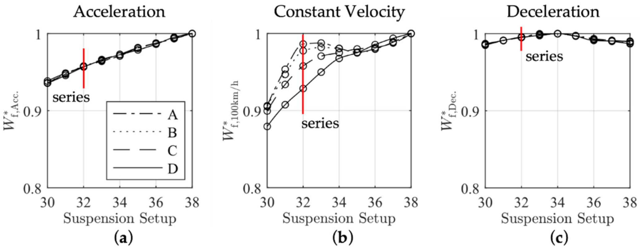
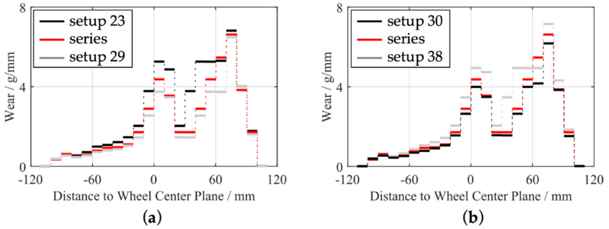
5.1. Variation of Initial Wheel Alignment
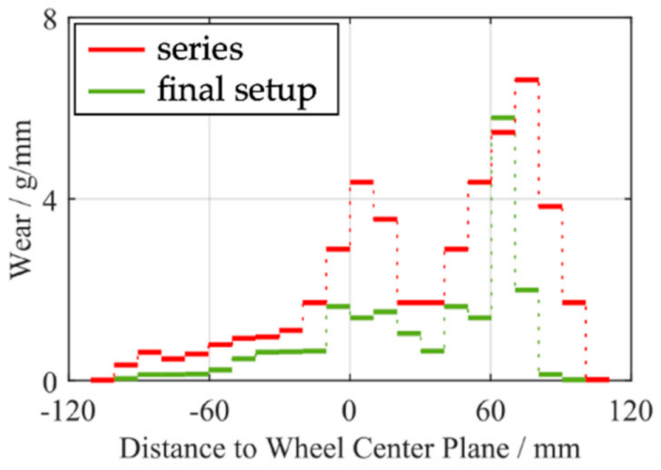
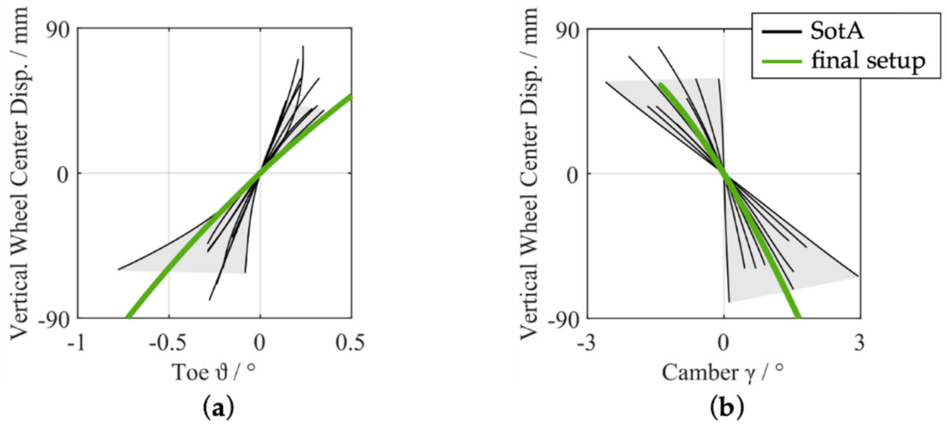
5.2. Variation of Kinematics of Wheel Travel
6. Conclusions
7. Summary and Future Work
Author Contributions
Funding
 .
.Institutional Review Board Statement
Informed Consent Statement
Data Availability Statement
Conflicts of Interest
References
- Diegmann, V.; Pfäfflin, F.; Wiegand, G.; Wursthorn, H. Maßnahmen Zur Reduzierung von Feinstaub Und Stickstoffdioxid; IVU Umwelt GmbH: Dessau, Germany, 2007. [Google Scholar]
- Willeke, H. CO2-Emission und Feinstaub in Verbindung mit Rollwiderstand von Reifen; DEKRA: Essen, Germany, 2008. [Google Scholar]
- Bundesministerium für Umwelt, Naturschutz und Nukleare Sicherheit (BMU). Klimaschutz in Zahlen: Fakten, Trends Und Impulse Deutscher Klimapolitik; Bundesministerium für Umwelt, Naturschutz und Nukleare Sicherheit (BMU): Berlin, Germany, 2019. [Google Scholar]
- Timmers, V.R.; Achten, P.A. Non-exhaust PM emissions from electric vehicles. Atmos. Environ. 2016, 134, 10–17. [Google Scholar] [CrossRef]
- OECD. Non-Exhaust Particulate Emissions from Road Transport; OECD: Paris, France, 2020. [Google Scholar]
- Boucher, J.; Friot, D. Primary Microplastics in the Oceans: A Global Evaluation of Sources; IUCN: Gland, Switzerland, 2017; p. 43. [Google Scholar]
- Bertling, J.; Bertling, R.; Hamann, L. Kunststoffe in Der Umwelt: Mikro- Und Makroplastik: Ursachen, Mengen, Umweltschicksale, Wirkungen, Lösungsansätze, Empfehlungen; Kurzfassung der Konsortialstudie, Fraunhofer-Institut für Umwelt-, Sicherheits- und Energietechnik; UMSICHT: Oberhausen, Germany, 2018. [Google Scholar] [CrossRef]
- Pottinger, M.G. Contact Patch (Footprint) Phenomena. In The Pneumatic Tire; National Highway Traffic Safety Administration NHTSA: Akron, OH, USA, 2006; pp. 231–285. [Google Scholar]
- Ersoy, M.; Gies, S. Fahrwerkhandbuch; J.B. Metzler: Berlin, Germany, 2017. [Google Scholar]
- Kohl, S.; Sextro, W.; Zuber, A. Benteler Vehicle Dynamics-Fahrdynamikentwicklung Basierend Auf Einer Neuen Auslegungstheorie. In 8 Tag Fahrwerks; RWTH Aachen University in Aachen: Aachen, Germany, 2012. [Google Scholar]
- Blundell, M.; Harty, D. Multibody Systems Approach to Vehicle Dynamics; Automotive Engineering Series; Elsevier Butterworth-Heinemann: Amsterdam, The Netherlands, 2004; ISBN 978-0-7506-5112-7. [Google Scholar]
- Kohl, S. Analyse Der Reibleistungsverteilung Im Reifenlatsch Unter Berücksichtigung Der Fahrwerkdynamik Eines Mehrlenkerachssystems Zur Bewertung Des Reifenverschleißes; Shaker Verlag: Aachen, Germany, 2019. [Google Scholar]
- Lupker, H.; Cheli, F.; Braghin, F.; Gelosa, E.; Keckman, A. Numerical Prediction of Car Tire Wear. Tire Sci. Technol. 2004, 32, 164–186. [Google Scholar] [CrossRef]
- Braghin, F.; Cheli, F.; Melzi, S.; Resta, F. Tyre Wear Model: Validation and Sensitivity Analysis. Meccanica 2006, 41, 143–156. [Google Scholar] [CrossRef]
- Gafvert, M.; Svendenius, J. A novel semi-empirical tyre model for combined slips. Veh. Syst. Dyn. 2005, 43, 351–384. [Google Scholar] [CrossRef]
- Sueoka, A.; Ryu, T.; Kondou, T.; Togashi, M.; Fujimoto, T. Polygonal Wear of Automobile Tire. JSME Int. J. Ser. C 1997, 40, 209–217. [Google Scholar] [CrossRef]
- Salminen, H. Parametrizing Tyre Wear Using a Brush Tyre Model. Ph.D. Thesis, KTH R. Institute Technology, Stockholm, Sweden, December 2014. [Google Scholar]
- Cho, J.C.; Jung, B.C. Prediction of Tread Pattern Wear by Explicit FEM. 33. J. Automob. Eng. 2014, 229, 197–213. [Google Scholar]
- Lee, S.W.; Jeong, K.M.; Kim, K.W.; Kim, J.H. Numerical Estimation of the Uneven Wear of Passenger Car Tires. World J. Eng. Technol. 2018, 6, 780–793. [Google Scholar] [CrossRef][Green Version]
- Tong, G.; Jin, X.; Road, C. Study on the Simulation of Radial Tire Wear Characteristics. Transp. Probl. 2012, 11, 11. [Google Scholar]
- Knisley, S. A Correlation Between Rolling Tire Contact Friction Energy and Indoor Tread Wear. Tire Sci. Technol. 2002, 30, 83–99. [Google Scholar] [CrossRef]
- Sakai, H. Friction and Wear of Tire Tread Rubber. Tire Sci. Technol. 1996, 24, 252–275. [Google Scholar] [CrossRef]
- Wright, C.; Pritchett, G.L.; Kuster, R.J.; Avouris, J.D. Laboratory Tire Wear Simulation Derived from Computer Modeling of Suspension Dynamics. Tire Sci. Technol. 1991, 19, 122–141. [Google Scholar] [CrossRef]
- Stalnaker, D.; Turner, J. Vehicle and Course Characterization Process for Indoor Tire Wear Simulation. Tire Sci. Technol. 2002, 30, 100–121. [Google Scholar] [CrossRef]
- Engel, D.; Biesse, F. Simulation based tire wear prediction by vehicle and tire model coupling. In 15. Internationale VDI-Tagung Reifen-Fahrwerk-Fahrbahn; VDI-Berichte: Berlin, Germany, 2015; ISBN 978-3-18-092241-6. [Google Scholar]
- Gipser, M.; Hofmann, G.F. Tire-The Market-Leading Physics-Based Tire Model; Esslingen University of Applied Sciences: Esslingen, Germany, 2018. [Google Scholar]
- ITWM. Scalable Tire Model for Full Vehicle Simulations; CDTire: Kaiserslautern, Germany, 2017. [Google Scholar]
- Fleischer, G. Energetische Methode Der Bestimmung Des Verschleisses. Schmierungstechnik 1973, 4, 269–274. [Google Scholar]
- Schütte, J.; Sextro, W. Model-Based Investigation of the Influence of Wheel Suspension Characteristics on Tire Wear. In Proceedings of the Advances in Dynamics of Vehicles on Roads and Tracks; Klomp, M., Bruzelius, F., Nielsen, J., Hillemyr, A., Eds.; Springer International Publishing: Cham, Switzerland, 2020; pp. 1760–1770. [Google Scholar]
- Schramm, D.; Hiller, M.; Bardini, R. Modellbildung und Simulation der Dynamik von Kraftfahrzeugen; Springer: Berlin/Heidelberg, Germany, 2013; ISBN 978-3-642-33887-8. [Google Scholar]
- DIN ISO 8855:2013-11. Straßenfahrzeuge-Fahrzeugdynamik und Fahrverhalten-Begriffe; Beuth Verlag Gmbh: Berlin, Germany, 2013; p. 51. [Google Scholar]
- Trzesniowski, M. Rennwagentechnik; Vieweg, Teubner Verlag: Wiesbaden, Germany, 2012; ISBN 978-3-8348-1779-2. [Google Scholar]
- Braess, H.-H.; Seiffert, U. Vieweg Handbuch Kraftfahrzeugtechnik; Springer Vieweg: Wiesbaden, Germany, 2013; ISBN 978-3-658-01690-6. [Google Scholar]
- Salzgitter Flachstahl GmbH Borlegierte Vergütungsstähle. Available online: https://www.salzgitter-flachstahl.de/de/produkte/warmgewalzte-produkte/stahlsorten/borlegierte-verguetungsstaehle.html (accessed on 1 August 2020).
- Craig, R.R.; Bampton, M.C.C. Coupling of substructures for dynamic analyses. AIAA J. 1968, 6, 1313–1319. [Google Scholar] [CrossRef]
- ZF Friedrichshafen AG WebCat-Online-Katalog-ZF Friedrichshafen AG, ZF Aftermarket. Available online: https://webcat.zf.com (accessed on 2 January 2021).
- Popov, V.L. Kontaktmechanik und Reibung; Springer: Berlin/Heidelberg, Germany, 2015; ISBN 978-3-662-45974-4. [Google Scholar]
- Burckhardt, M.; Burg, H. Berechnung Und Rekonstruktion Des Bremsverhaltens von PKW; Information Ambs GmbH: Kippenheim, Germany, 1988; ISBN 978-3-88550-025-4. [Google Scholar]
- Schütte, J.; Sextro, W.; Kohl, S. Halbachsprüfstand Zur Kinematischen, Elastokinematischen Und Dynamischen Charakterisierung von Radaufhängungen. Fachtag. Mechatronik 2019, 1, 103–108. [Google Scholar]
- Cosin Scientific Software AG. F Tire-Flexible Structure Tire Model: Modelization and Parameter Specification; Cosin Scientific Software AG: Munchen, Germany, 2021. [Google Scholar]
- Gipser, M. F Tire: A Physically Based Tire Model for Handling, Ride, and Durability Part 2: Modelization. SAE Int. J. Passeng. Cars Mech. Syst. 2014, 7, 231–243. [Google Scholar]
- Cosin Scientific Software AG Cosin Scientific Software. Available online: https://www.cosin.eu (accessed on 1 July 2020).
- MSC Adams. Help—Road Models, MSC Software. 2020.
- International Organization for Standardization ISO 8608:2016-11. Mechanical Vibration Road Surface Profiles Reporting of Measured Data; International Organization Standardization: Geneva, Switzerland, 2016. [Google Scholar]
- Braun, H.; Hellenbroich, T. Messergebnisse von Strassenunebenheiten. VDI-Berichte 1991, 877, 47–80. [Google Scholar]
- Kummer, H.W. Unified Theory of Rubber and Tire Friction; B-94; Pennsylvania State Univ: University Park, PA, USA, 1966. [Google Scholar]
- Bachmann, T. Literaturrecherche Zum Reibwert Zwischen Reifen Und Fahrbahn; Berichte aus dem Fachgebiet Fahrzeugtechnik der TH Darmstadt; VDI-Verlag: Düsseldorf, Germany, 1996; ISBN 3-18-328612-2. [Google Scholar]
- Moldenhauer, P. Modellierung Und Simulation Der Dynamik Und Des Kontakts von Reifenprofilblöcken; VDI-Verlag: Düsseldorf, Germany, 2010. [Google Scholar]
- Sextro, W. Dynamical Contact Problems with Friction Models, Methods, Experiments and Applications; Springer: Berlin/Heidelberg, Germany, 2007; ISBN 978-3-540-45317-8. [Google Scholar]
- Glaser, H.; Rossié, T.; Rüger, J.; Conrad, T.; Wagner, R. Das Fahrwerk. ATZextra 2010, 15, 32–37. [Google Scholar] [CrossRef]
- Hudler, R.; Leitner, D.I.W.; Krome, H.; Steigerwald, A.; Fischer, D.I.S. Die Achsen des neuen Audi A4. ATZextra 2007, 12, 104–113. [Google Scholar] [CrossRef]
- Audi Q3: Entwicklung und Technik; Rudolph, H.-J., Ed.; ATZ/MTZ-Typenbuch; Springer Vieweg: Wiesbaden, Germany, 2013; ISBN 978-3-658-00852-9. [Google Scholar]
- Hoffmann, J. Potentiale Einer Aktiven Achskinematik zur Optimierung des Fahrverhaltens; Schriftenreihe des Instituts für Fahrzeugtechnik, TU Braunschweig; Shaker Verlag: Aachen, Germany, 2016; ISBN 978-3-8440-4554-3. [Google Scholar]


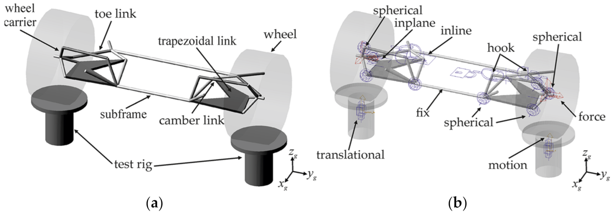
| Number of Bodies: | = 11 | |
| Number of joints: | = 19 | |
| Degrees of freedom—fix joint | = 0 | (3x) |
| Degrees of freedom—hook joint | = 2 | (4x) |
| Degrees of freedom—spherical joint | = 3 | (8x) |
| Degrees of freedom—inline joint | = 4 | (2x) |
| Degrees of freedom—inplane joint | = 5 | (2x) |
| Part | Material | Density/g/cm3 | Young’s Modulus/GPa | Poisson’s Ratio |
|---|---|---|---|---|
| Toe link | AlSi1MgMnT6 | 2.7 | 70 | 0.33 |
| Camber link | AlSi1MgMnT6 | 2.7 | 70 | 0.33 |
| Trapezoidal link | AlSi1MgMnT6 | 2.7 | 70 | 0.33 |
| Wheel carrier | AlSi7Mg0,3 | 2.68 | 74 | 0.33 |
| Stabilizer | 26MnB5/34MnB5 | 7.85 | 210 | 0.30 |
| Stabilizer link | PA 6.6 GF57 | 1.681 | 19.95 | 0.38 |
| Size | 245/40ZR18 |
| Inflation pressure | 270 kPa |
| Number of belt segments | 88 |
| Number of tread blocks per belt segment | 44 |
| Number of tread strips | 22 |
| Suspension Setup | ||
|---|---|---|
| 1 | −20′ | −1° 20′ |
| 2 | −14′ | −1° 20′ |
| 3 | −8′ | −1° 20′ |
| 4 | −2′ | −1° 20′ |
| 5 | 4′ | −1° 20′ |
| 6 (series) | 10′ | −1° 20′ |
| 7 | 16′ | −1° 20′ |
| 8 | 22′ | −1° 20′ |
| 9 | 28′ | −1° 20′ |
| 10 | 34′ | −1° 20′ |
| 11 | 40′ | −1° 20′ |
| Suspension Setup | ||
|---|---|---|
| 12 | 10′ | 1° 20′ |
| 13 | 10′ | 48′ |
| 14 | 10′ | 16′ |
| 15 | 10′ | −16′ |
| 16 | 10′ | −48′ |
| 17 (series) | 10′ | −1° 20′ |
| 18 | 10′ | −1° 52′ |
| 19 | 10′ | −2° 24′ |
| 20 | 10′ | −2° 56′ |
| 21 | 10′ | −3° 28′ |
| 22 | 10′ | −4° |
| Suspension Setup | Tire Wear/g | Tire Wear Reduction/% |
|---|---|---|
| Series | 470 | - |
| Setup 29 | 419 | 10.9 |
| Setup 30 | 428 | 8.9 |
| Final Setup | 204 | 56.6 |
Publisher’s Note: MDPI stays neutral with regard to jurisdictional claims in published maps and institutional affiliations. |
© 2021 by the authors. Licensee MDPI, Basel, Switzerland. This article is an open access article distributed under the terms and conditions of the Creative Commons Attribution (CC BY) license (https://creativecommons.org/licenses/by/4.0/).
Share and Cite
Schütte, J.; Sextro, W. Tire Wear Reduction Based on an Extended Multibody Rear Axle Model. Vehicles 2021, 3, 233-256. https://doi.org/10.3390/vehicles3020015
Schütte J, Sextro W. Tire Wear Reduction Based on an Extended Multibody Rear Axle Model. Vehicles. 2021; 3(2):233-256. https://doi.org/10.3390/vehicles3020015
Chicago/Turabian StyleSchütte, Jan, and Walter Sextro. 2021. "Tire Wear Reduction Based on an Extended Multibody Rear Axle Model" Vehicles 3, no. 2: 233-256. https://doi.org/10.3390/vehicles3020015
APA StyleSchütte, J., & Sextro, W. (2021). Tire Wear Reduction Based on an Extended Multibody Rear Axle Model. Vehicles, 3(2), 233-256. https://doi.org/10.3390/vehicles3020015