RTOB SLAM: Real-Time Onboard Laser-Based Localization and Mapping

Abstract

RTOB-SLAM is a new low-computation framework for real-time onboard simultaneous localization and mapping (SLAM) and obstacle avoidance for autonomous vehicles. A low-resolution 2D laser scanner is used and a small form-factor computer perform all computations onboard. The SLAM process is based on laser scan matching with the iterative closest point technique to estimate the vehicle’s current position by aligning the new scan with the map. This paper describes a new method which uses only a small subsample of the global map for scan matching, which improves the performance and allows for a map to adapt to a dynamic environment by partly forgetting the past. A detailed comparison between this method and current state-of-the-art SLAM frameworks is given, together with a methodology to choose the parameters of the RTOB-SLAM. The RTOB-SLAM has been implemented in ROS and perform well in various simulations and real experiments.

1. Introduction

1.1. Context

Over the last couple of years, ground and air autonomous vehicles have become incredibly popular in academia and industry. For position estimation, most of them rely completely on GPS and their inertial sensors, som even millimeter radar waves [1]. These sensors give an estimate of the position but do not provide any information on the environment, and have limited accuracy -in particular for GPS. To overcome both limitations, cameras [2,3] and laser scanners are commonly used to sense the surroundings. This data can be used for simultaneous localization and mapping (SLAM) and obstacle avoidance [4], improving both the operational safety and the quality of the position estimates.

While fast and high-resolution cameras are relatively small and light-weight, the post-processing of the data requires powerful computers which are usually unsuited aboard a lightweight autonomous vehicle. This makes such vehicles dependent on a powerful ground-station computer. Current 3D laser scanners are too heavy, bulky and expensive for the use aboard a small unmanned aerial vehicle (UAV). Many 2D laser scanners present a good compromise, as they give information on the surroundings, provide a tractable amount of data, are lightweight and low cost. It is also possible to convert a 2D laser scanner into a true 3D laser scanner by adding an additional axis of rotation as we showed in our previous work [5]. For a safe operation in possibly cluttered indoor and outdoor environments, the information on the surroundings can additionally be used for obstacle avoidance. The next paragraph reviews commonly-used methods for SLAM and obstacle avoidance.

1.2. Related Work

SLAM is about constructing a map of an unknown environment and determining the vehicle’s position in this environment simultaneously. To overcome the challenge of performing the SLAM task in real-time with limited computational resources [6], different approaches can be found in literature. They can broadly be divided in two groups: (1) One group tries to simplify the SLAM problem by making assumptions about the environment. (2) The other group tries to simplify or speed up the algorithm while relaxing the assumptions on the environment. A prominent algorithm falling into the first group is OrthoSLAM. Nguyen et al. [7] developed OrthoSLAM in 2006, which assumes that most walls in an indoor environment are straight and either parallel or orthogonal to each other. The position is then calculated only based on the orthogonal parts of the environment, which reduces the computational complexity significantly. Successful real-time onboard implementations for UAVs are presented by Alpen et al. [8,9]. However, this algorithm is only applicable, when the assumption of an orthogonal environment mostly holds.

Almost all contributions that fall in the second category rely on some variant of the iterative closest point (ICP) algorithm. This algorithm iteratively aligns a set of points with a given reference by minimizing some cost function (e.g., the distance between all nearest neighbors). This is computationally expensive but has the advantage of not constraining the UAV to an environment that fulfills specific assumptions. The point-to-line matching extension PL-ICP to the vanilla ICP method has been proposed in [10]. An improved version has been successfully applied in [11] to an autonomous quadrotor in a static environment. For small UAVs variants of the ICP algorithm which use occupancy grids and modified cost functions have been shown to work well for static scenes [12,13]. However, these implementations cannot adapt to scenes that change quickly. This is because an occupancy grid does not store information about the scan time, it only stores the spatial information. The space is partitioned into a grid and the occupancy grid counts how often a laser measurement detects an object in each of the cells of the grid. The laser scan is then matched with the mean value of the occupancy grid. Consequently, this technique is ideal to minimize the influence of outliers, but if the environment changes, this will not be detected quickly. Another approach next to ICP is the probability-based scan matching presented by Grzonka et al. [14]. However, due to the high demand of computational power, this approach needs to run partly on an offboard computer. A computationally less demanding probability-based framework is TinySLAM [15]. This has been adapted for aerial vehicles and successfully tested on a small UAV in static indoor environments [16].

SLAM is not only used for small UAVs but also for a wide range of ground-based robots. An embedded real-time SLAM approach able to adapt to changing environment is found in [17] in the case of a ground robot. For such applications high computational demand is usually less critical since the additional weight of a more powerful computer is accomodated. Often the main focus is not real-time processing but creating the most accurate map possible. Algorithms relying on occupancy-grid-based ICP are most commonly used. Two prominent examples are cartographer [18] and gmapping [19].

Table 1. Comparison between RTOB-SLAM and two widely used algorithms.

	Arbitrary Environment	Real-Time Onboard	Dynamic Environment
RTOB-SLAM	Yes	Yes	Yes
OrthoSLAM	No	Yes	No
Cartographer	Yes	Yes	(Yes)

shows a comparison between RTOB-SLAM and the methods mentioned above. OrthoSLAM is the least computationally-demanding algorithm but it requires a special environment. Cartographer on the other hand is a highly optimized and very complex algorithm that is able to run in real-time on most hardware. However, it is based on occupancy grids and is thus primarily optimized for static environments. RTOB-SLAM is able to run onboard a vehicle with a small form-factor PC (e.g., Intel UPBoard: 4 × 1.44 GHz) while allowing for arbitrary, possibly dynamic environments.

1.3. Contributions

The main contribution of this work is the design of a new computationally lightweight framework for simultaneous localization and mapping (SLAM) as well as obstacle avoidance solely with data available from a 2D laser scanner, in real-time and completely aboard the vehicle. The resulting algorithm has thus been named RTOB-SLAM as the acronym for real-time on-board SLAM. This method proves to perform particularly well with very sparse data, therefore, this paper also shows its applicability to a low-cost 3D laser scanner developed in [5]. RTOB-SLAM uses a fast scan matching technique based on iterative closest point (ICP) matching. This method works in nearly any arbitrary dynamic environment and it can explore new territory and return to already visited areas with no visible loop-closing issue, i.e., the map stays consistent if the vehicle revisits an area that it already mapped. No active measures against loop-closure problems (e.g., bundle adjustment and optimization [20]) need to be implemented because—in contrast to other methods using submaps—the scans are always matched against a single, global, and therefore consistent, map. An in-depth treatment on how the RTOB-SLAM parameters need to be chosen is presented. In addition, the paper provides a detailed comparison between RTOB-SLAM and the current state-of-the art of SLAM frameworks. Last, a collision avoidance is developed around RTOB-SLAM to efficiently and safely map an unknown environment in a semi-autonomous manner. This means that a human pilot commands the “general” flight direction, but the vehicle will autonomously avoid obstacles detected during the SLAM process.

The next section describes the newly developed RTOB-SLAM technique and its performance evaluated in simulated and real-life cases. The last part of the paper shows the effectiveness of the algorithm during real-flight experiments of a multirotor helicopter, performing semi-autonomous exploration.

2. Localization and Mapping

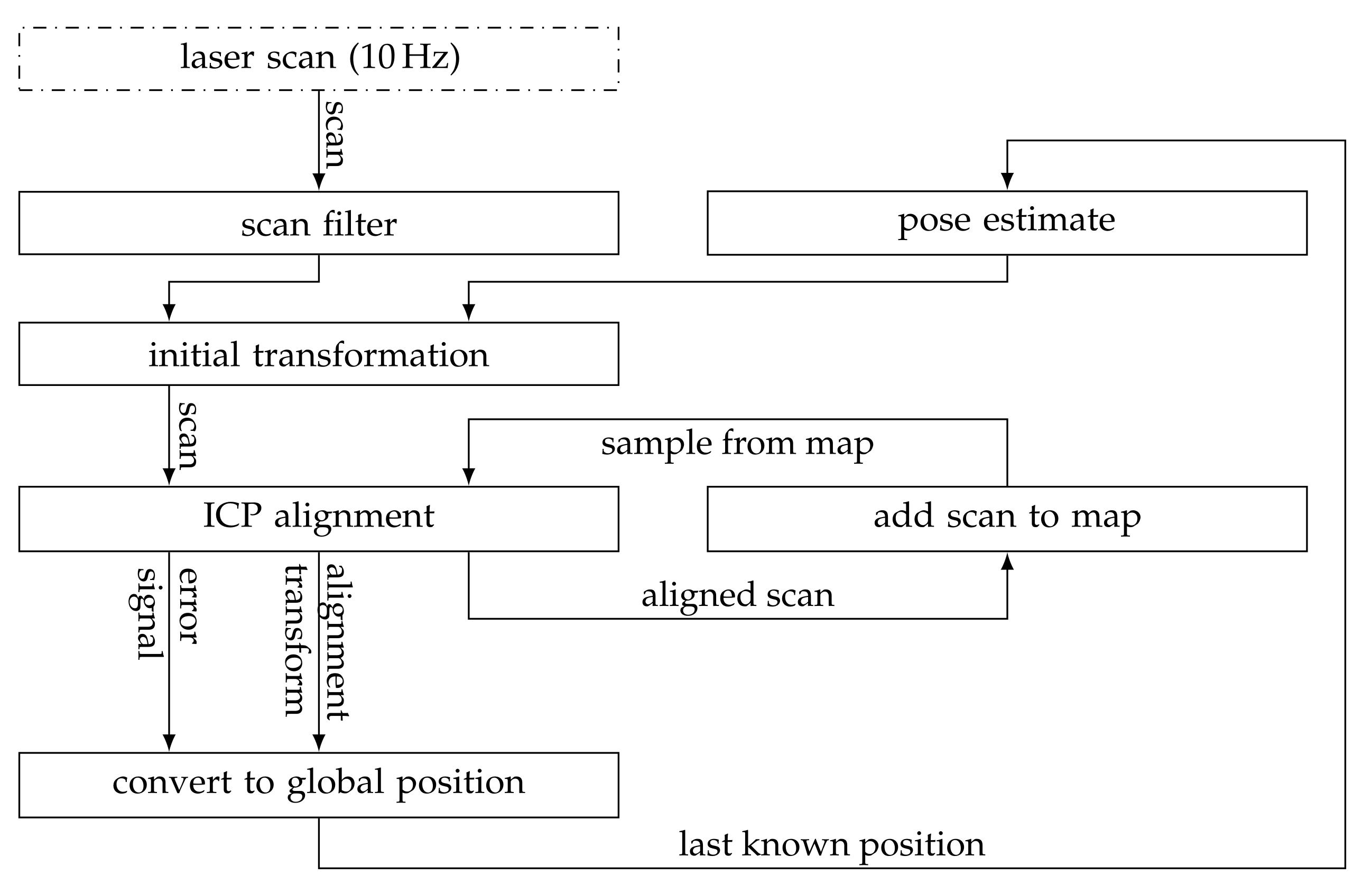
The methods described above are either not capable of onboard real-time applications or have significant difficulties in adapting to a changing environment. This section first describes the newly developed method in detail, which (1) is able to run on an onboard small form-factor computer in real-time and (2) can be tuned to adapt to a changing environment. Then experimental results are shown. It is important to recognize that even seemingly static environments turn out to be dynamic when a 2D representation is used. Indeed, depending on the altitude of the vehicle, the environment can look differently, e.g., a chair is only visible at lower altitudes but suddenly ‘disappears’ as the vehicle climbs. Hence, even static environments can look like dynamic ones to the vehicle and thus adapting to a dynamic environment is very important. Otherwise the localization of the UAV very likely fails which can eventually lead to a crash.

2.1. Scan Alignment

Figure 1 gives an overview of the developed method and Figure 2 shows a simple example. The laser scanner sends a new scan (Figure 2a). The laser scan is filtered to remove outliers and is pre-aligned with the map (Figure 2b). Then the ICP technique is used to refine this initial alignment (Figure 2c). In a final step the aligned scan is added to the map and the initial alignment is combined with the refined alignment to obtain the global position of the vehicle.

2.1.1. Scan Filter

In this step, outliers and invalid scan points are removed. A laser scan is the collection of the scan points $s_i$, thus the filtered scan $\mathcal{S}$ can be written as:

$$\mathcal{S}=\left\{s_i|d_i\in \left[d_{\min },d_{\max }\right]\right\}$$

(1)

where $d_i$ is the distance of the i-th scan point and $[d_{\min },d_{\max }]$ is the measurement range of the laser scanner. This simple thresholding method is fast, robust and reliable.

2.1.2. Initial Alignment

Once the laser-scan points have been filtered, the laser scan needs pre-alignment with the map of the environment which is known from the previous time-step (for the first scan, this step is skipped). Because the ICP-alignment method can fail due to local minima of the cost function, a good initial alignment of the scan is necessary. This is pictured in Figure 2a where no meaningful nearest neighbor associations are possible. Only when the scan is pre-aligned as shown in Figure 2b can point-to-point matching techniques be successful. This implementation needs an initial alignment accuracy of 30 cm and 5 degrees (see maximum correspondence distance, section III-C).

Two different possibilities exist for the initial alignment: (1) If the vehicle has no other sensors for navigation than the laser scanner (i.e., no optical flow, no IMU) the position from the last ICP alignment can be used. (2) If additional sensors are available, this information can be fused with a Kalman filter to obtain an improved position estimate.

Let x and y denote the coordinates of the vehicle’s estimated position and $\psi$ the yaw angle, then the initial alignment can be written in homogeneous coordinates as:

$${\mathcal{S}}^{\prime }=\left\{{\mathbf{T}}_{\mathrm{init}}{s}_i|\forall s_i\in \mathcal{S}\right\}$$

(2)

where the transformation matrix ${\mathbf{T}}_{\mathrm{init}}$ is given by

$$\begin{array}{c}\hfill {\mathbf{T}}_{\mathrm{init}}=\left(\begin{array}{cccc}cos\psi & -sin\psi & 0& x\\ sin\psi & cos\psi & 0& y\\ 0& 0& 1& 0\\ 0& 0& 0& 1\end{array}\right)\end{array}$$

(3)

This transformation does not account for pitch/roll motions of the vehicle. For small tilt-angles <5 deg the error is below 0.5% and thus comparable to the measurement accuracy of the used laser scanner. If the vehicle is allowed to tilt more (more aggressive maneuvers), the laser scanner would often scan the ceiling and the floor or perceive obstacles at different heights in most real-life applications. Therefore, the pitch and roll angles need to be very small and the resulting distortion of the scans is negligible.

2.1.3. ICP Alignment

This step is the most important step in the RTOB-SLAM procedure, since the laser scan will be precisely aligned with the map (reference) as shown in Figure 2c. The standard ICP technique involves three steps that are performed iteratively until some convergence criteria are met:

• For each point in the scan, find the nearest neighbor point in the map.
• Find the transformation ${\mathbf{T}}_{\mathrm{ICP}}$ that minimizes the cost function J, where J is given by the sum of all point-to-point distances. The cost is minimized by solving a least-squares system. The commonly used Point-Cloud-Library uses the highly efficient singular value decomposition for this [21].
• Transform all points with ${\mathbf{T}}_{\mathrm{ICP}}$ and iterate until the problem converged (see Section 2.3).

After converging, the overall error can be checked and—if the scan is aligned well—it is added to the map. The mean of the squared nearest-neighbor distances is used as a measure of the alignment error. This is especially convenient because this measure is already calculated during the ICP-iteration. If the overall error is too large, the map is not updated during this cycle.

2.1.4. Update and Output

In the last step of the RTOB-SLAM algorithm, the pose of the vehicle is calculated from the two transformations ${\mathbf{T}}_{\mathrm{init}}$ and ${\mathbf{T}}_{\mathrm{ICP}}$. It is important to note that a straightforward multiplication of the two matrices does not lead to the correct result due to the homogeneous coordinates. The two shifts in x and y need to be added while only the rotational part of the matrices can be multiplied. Hence the final transformation is given by:

$$\mathbf{T}=\left(\begin{array}{cccc}cos{\psi }^{\prime }& -sin{\psi }^{\prime }& 0& x^{\prime }\\ sin{\psi }^{\prime }& cos{\psi }^{\prime }& 0& y^{\prime }\\ 0& 0& 1& 0\\ 0& 0& 0& 1\end{array}\right)\mathrm{with}\begin{array}{c}{\psi }^{\prime }={\psi }_{\mathrm{init}}+{\psi }_{\mathrm{ICP}}\hfill \\ x^{\prime }=x_{\mathrm{init}}+x_{\mathrm{ICP}}\hfill \\ y^{\prime }=y_{\mathrm{init}}+y_{\mathrm{ICP}}\hfill \end{array}$$

(4)

2.2. Position Estimation

The algorithm outputs the matrix $\mathbf{T}$ calculated using (4). The position of the vehicle is obtained by taking the first two rows of the last column, i.e., by extracting $x^{\prime }$ and $y^{\prime }$. The coordinates are in the global coordinate frame. This means that $x^{\prime }$ and $y^{\prime }$ capture the movement of the vehicle relative to where it started the flight. If one needs to use a different global north-east-down (NED) coordinate system, this can be realized by multiplying $\mathbf{T}$ with another transformation matrix.

2.3. ICP Alignment Details

Due to the limited computational resources of the onboard computer, the SLAM framework must be as efficient as possible. Critical for the overall runtime is a fast ICP implementation. Therefore, it relies on the Point Cloud Library (PCL) [22] which is a highly optimized C++ template library, specifically designed to handle large point clouds in two or three dimensions. Not only a fast performance is required, but also a nearly constant runtime, since the framework must run in real-time and a worst-case execution time (WCET) should be known at least empirically.

2.3.1. Number of Iterations

The PCL-ICP has some tunable options including a parameter for maximum iterations, two convergence parameters epsilon and a maximum correspondence distance parameter. As soon as the algorithm finds that the improvement between two consecutive iterations did not yield any significant decrease (less then epsilon), it outputs the result and stops. To ensure constant runtimes, it is important that the algorithm always does the same number of iterations and never meets the convergence criteria. Therefore, the two epsilon-parameters are set to very small numbers (around $1\times {10}^{-9}$). Hence the algorithm performs always the maximum number of iterations because the decrease of the cost will always be greater than this small number. The epsilon parameters could also be set to a meaningful value because constant runtimes are only a special case of a known WCET. Because this would make the tuning process more complicated and since it is not necessary to reserve some unused computational power, the convergence parameters are set to very small values. The maximum number of iterations should be chosen as high as possible because this improves the accuracy of the alignment. The real-time constraint however places an upper bound on the runtime.

The maximum correspondence distance specifies how far two neighbouring points can be apart and is directly related to the required initial alignment accuracy. Larger values increase the chance of ICP to fail due to a local minimum but also require a less precise initial alignment.

2.3.2. Sampling from the Map

A major problem for the ICP technique is that its runtime strongly depends on the number of points in the reference map. An exhaustive nearest neighbor search that does not use approximations has a runtime of $\mathcal{O}\left(n\right)$, where n is the number of points in the reference map that grows over time. Hence some kind of downsampling of the map is needed as shown in Figure 1. A common solution is to use occupancy grids which can be implemented very efficiently but they cannot adapt to dynamic environments quickly. This section presents a different and new approach which is efficient and allows for accurate localization in a changing environment.

The new idea is to use a probability-based approach to downsample the map before the current scan is aligned with it. Let $\mathcal{P}\left(s\right)$ denote the probability that the scan point s obtained at time t is included in the reference map.

$$\mathcal{P}\left(s\right)=\left\{\begin{array}{cc}p\left(t\right)\hfill & t\in [t_{\min },t_{\max }]\hfill \\ 0\hfill & \mathrm{otherwise}\hfill \end{array}\right.$$

(5)

By choosing the probability density function $p\left(t\right)$ and the times $t_{\min }$ and $t_{\max }$, the behavior of the mapping can be influenced. Each time a new laser scan needs to be aligned, a new sample of points is drawn. The number of points is fixed and needs to be optimized empirically. The best results are obtained when the largest, computationally feasible number is chosen, which is 3600 in this work. Due to the constant number of points in the randomly sampled reference, the RTOB-SLAM does not get slower if the global map gets larger.

The following paragraph discusses the most simple choice for $p\left(t\right)$ but this function can be chosen almost arbitrarily. Let $p\left(t\right)=\mathrm{uni}(t_{\min },t_{\max })$ be a uniform distribution on the interval $[t_{\min },t_{\max }]$. Let $t_i$ denote the time at which the i-th point was scanned.

• Case a): If $t_{\min }=0$ and $t_{\max }=max\left(t_i\right)$ the reference map is a random sample drawn from the whole past. This is very close to an occupancy grid.
• Case b): If $t_{\min }>0$ and $t_{\max }=max\left(t_i\right)$ the reference map can be based—depending on the choice of $t_{\min }$— on the most recent observations. If the environment changed at time $t_{\mathrm{change}}$ where $t_{\mathrm{change}}$ is less than $t_{\min }$ the RTOB-SLAM performance will not be influenced by this change.

When flying in an environment that constantly changes (compared to one change at a certain time $t_{\min }$) it is sensible to chose $t_{\min }=t-t_{\mathrm{offset}}$ and $t_{\max }=t$ where t is the current time and $t_{\mathrm{offset}}$ is some fixed offset time.

Not only uniform distributions are possible, but also for example exponential forgetting can be realised with a Poisson probability density function $p\left(t\right)=\lambda {\mathrm{e}}^{-\lambda t}$. Even more advanced choices for $p\left(t\right)$ are possible. For example, one could use a probability density that depends not only on time but also on space. Then the reference only consists of points that were sampled recently and that are located in the vicinity of the vehicle.

2.3.3. Loop-Closure in Static Environments

Although the random sampling speeds up the process significantly, it can lead to loop-closing problems. When the support region of $p\left(t\right)$ is only a subset of the total flight time, it is possible that the vehicle ‘rediscovers’ a region which it already explored which can result in an inconsistent final map. Therefore it is important to choose $p\left(t\right)$ correctly when larger areas are mapped. Let $f:t\mapsto (x,y)$ denote the vehicle’s time-parametrized trajectory. To avoid loop-closing problems, a scan obtained at a certain position $(x^{*},y^{*})$ needs to be matched against a reference containing a random subsample of all the information about this region to avoid ‘rediscovering’ the region. First, the set of all past times ${\mathcal{S}}_{t^{*}}$ where the vehicle was close to the current location (within $\Delta x$, $\Delta y$ offset) needs to be determined: find ${\mathcal{S}}_{t^{*}}$ such that

$$f\left(t^{*}\right)\in [x^{*}-\Delta x,x^{*}+\Delta x]\times [y^{*}-\Delta y,y^{*}+\Delta y]\forall t^{*}\in {\mathcal{S}}_{t^{*}}$$

From this, one possible choice for the probability density is the sum of Gaussians centered at each of the times $t^{*}$, i.e.,

$$p\left(t\right)=\frac{1}{|{\mathcal{S}}_{t^{*}}|}\sum _{t^{*}\in {\mathcal{S}}_{t^{*}}}\frac{1}{\sigma \sqrt{2\pi }}exp{\left(-\frac{t-t^{*}}{\sqrt{2}\sigma }\right)}^2$$

where $\sigma$ is a tuning parameter. A larger $\sigma$ results in a smoother $p\left(t\right)$. Choosing $\sigma =1$ and $\Delta x=\Delta y=r/\sqrt{2}$ where r is the range of the LIDAR will produce satisfactory results in most applications. For dynamic environments, exponential forgetting can be incorporated as well. This particular choice of $p\left(t\right)$ guarantees that no loop-closure problems appear, as long as the ‘loop error’ is smaller than the maximum correspondence distance of the ICP. The loop error is defined as the localization error for a closed trajectory where $p\left(t\right)=\mathrm{uni}(t_{\min },t_{\max })$ was chosen as discussed in the previous section.

The possibility to choose a special $p\left(t\right)$ that possesses certain desired characteristics is one of the benefits of the RTOB-SLAM. Algorithms like Cartographer use pose-graph-based bundle adjustment to prevent loop-closing problems which is computationally expensive and gets slower if the map grows because the pose-graph grows. The approach RTOB-SLAM uses, namely to construct one global map which is never adjusted or corrected, scales better: the reference map is a subsample with a constant number of points and thus the ICP scan-matching does not get slower over time. Pose-graph optimization is more robust but using a random subsample with a suitable probability density function is computationally less demanding and appropriate for onboard SLAM on a UAV.

3. Results

3.1. Experimental Setup

The RTOB-SLAM method described in Section 2.1 has been experimentally verified in simulation and through real-life experiments. The algorithms are implemented in C++ and rely on the ROS (Robot Operating System) for interfacing the laser scanner and the flight controller of the vehicle. The ICP scan matching is done with the Point Cloud Library (PCL).

For the real-life experiments the hexacopter shown in Figure 3 with a ‘spanwidth’ of 0.9 m was used. It is controlled by the Pixhawk autopilot, which is common in academia. The vehicle is equipped with a RPLidar A2M4 2D laser scanner which has a resolution of 1 degree, a sampling frequency of 10 Hz and a range of 6 m. The RTOB-SLAM algorithm runs aboard the drone on an Intel UPBoard (small form-factor computer with a 4 × 1.44 GHz CPU). The vehicle is—apart from position commands issued by the pilot —fully autonomous.

The indoor flight tests were conducted inside the institute’s room which has a size of 4.8 m by 3.7 m. The windows of the room were covered with cardboard to make them visible for the laser scanner. The outdoor flight tests were conducted in a residential neighborhood with a very mild wind (<1 m/s) present.

3.2. Experimental Results

3.2.1. Simulation

To simulate the vehicle, the laser scanner and the environment around it, the open-source framework Gazebo (http://gazebosim.org/, accessed on 10 September 2021) is used which can be easily interfaced with ROS. A major advantage of the proposed RTOB-SLAM technique over other commonly used methods like OrthoSLAM [7] is that localization is possible in an environment with arbitrary shapes. To demonstrate this, a simulated flight was conducted in an environment which consists of three large cylinders. Figure 4 shows the map generated during this flight (blue) and the flight path of the vehicle (red). This simulation proves that the accuracy of the alignment does not depend on the shape of the objects around the vehicle.

The simulation experiments highlight a very convenient property of the proposed setup: all sensors (laser scanner, laser altimeter) can be simulated accurately with a very small simulation to real-world gap. This allows fine-tuning of RTOB-SLAM in simulation and zero-shot transfer to outdoor experiments was observed. The biggest difference between simulation and real-world comes from the complex aerodynamics of multirotor aerial vehicles, especially in confined spaces. However, a well-tuned low-level flight controller abstracts this away from RTOB-SLAM.

3.2.2. Indoor Experiments

Tight indoor environments are challenging for a hexacopter because much turbulence is present and hence the position changes quickly and unpredictably. Figure 5 shows the map and the flight path generated during a three-minute flight inside a room at the institute. The room’s heater (shown in green) is not visible at all altitudes. This flight demonstrates the vehicle’s ability

• to map indoor environments
• to hover stationary in the presence of severe turbulence

This experiment also proves that an update rate of 10 Hz for the position estimation is fast enough even in challenging flight conditions as long as the vehicle’s ground speed is relatively low. If speeds above 2–3 m/s are desired, a scanner with a higher update rate and greater range is needed. If the vehicle only needs to counteract the strong turbulence that it creates in tight indoor environments the laser’s update rate is sufficient.

The dataset generated during this flight was also analyzed using Cartographer. This flight has been chosen because the heater is the only dynamic environment in this dataset. The map that Cartographer generated was visually identical to the one generated with RTOB-SLAM but Cartographer generated the map about three times faster than our algorithm.

3.2.3. Outdoor Experiments

To demonstrate the versatility of the proposed framework a flight in a larger outdoor environment (without GPS) was made. The generated map and the estimated flight path are depicted in Figure 6 and clearly show the following properties of the method:

• It can cope with a dynamic environment: the side wall and the trash bin are not visible at higher altitudes.
• It can discover new areas: everything outside of the garage was not visible when the flight started
• When revisiting areas that have already been discovered, no loop-closing issues are visible.

4. Discussion and Conclusions

In this work, a real-time onboard SLAM algorithm named RTOB-SLAM has been developed to enable simultaneous localization and mapping with a low-resolution 2D laser scanner running on a small form-factor computer. This approach is suitable for (a) light-weight vehicle which possess limited computing power such as autonomous aerial vehicles, and also for (b) ground vehicles for which power consumption is a concern.

This new method is based on ICP scan matching and introduced the use of probability-density function in order to obtain a subsample of the global two-dimensional map, which is used for scan-matching. Using a two-dimensional map yields a reduced computational demand, however there are inherent limitations. Our RTOB-SLAM can only be used if the environment shows at least some ‘consistency’ across different height levels. Objects becoming visible at a certain level are not problematic due to the robustness of ICP, but if the environment suddenly changes completely at a height level, localization will fail.

In contrast to other real-time methods, it makes no assumption about the shape and configuration of the environment, it can cope with changing surroundings and scales well for larger maps. Experiments with a small aerial vehicle successfully demonstrated the capability of the RTOB-SLAM in real-life indoor and outdoor settings.

References

1. Li, Y.; Liu, Y.; Wang, Y.; Lin, Y.; Shen, W. The Millimeter-Wave Radar SLAM Assisted by the RCS Feature of the Target and IMU. Sensors 2020, 20, 5421. [Google Scholar] [CrossRef] [PubMed]
2. Liu, Y.; Chen, Z.; Zheng, W.; Wang, H.; Liu, J. Monocular Visual-Inertial SLAM: Continuous Preintegration and Reliable Initialization. Sensors 2017, 17, 2613. [Google Scholar] [CrossRef] [PubMed] [Green Version]
3. Munguía, R.; Urzua, S.; Bolea, Y.; Grau, A. Vision-Based SLAM System for Unmanned Aerial Vehicles. Sensors 2016, 16, 372. [Google Scholar] [CrossRef] [PubMed] [Green Version]
4. López, E.; García, S.; Barea, R.; Bergasa, L.M.; Molinos, E.J.; Arroyo, R.; Romera, E.; Pardo, S. A Multi-Sensorial Simultaneous Localization and Mapping (SLAM) System for Low-Cost Micro Aerial Vehicles in GPS-Denied Environments. Sensors 2017, 17, 802. [Google Scholar] [CrossRef] [PubMed]
5. Bauersfeld, L.; Ducard, G. Low-cost 3D Laser Design and Evaluation with Mapping Techniques Review. In Proceedings of the 2019 IEEE Sensors Applications Symposium (SAS), Sophia Antipolis, France, 11–13 March 2019; pp. 81–86. [Google Scholar]
6. Krul, S.; Pantos, C.; Frangulea, M.; Valente, J. Visual SLAM for Indoor Livestock and Farming Using a Small Drone with a Monocular Camera: A Feasibility Study. Drones 2021, 5, 41. [Google Scholar] [CrossRef]
7. Nguyen, V.; Harati, A.; Martinelli, A.; Siegwart, R. Orthogonal SLAM: A Step toward Lightweight Indoor Autonomous Navigation. In Proceedings of the 2006 IEEE/RSJ International Conference on Intelligent Robots and Systems, Beijing, China, 9–15 October 2006; pp. 5007–5012. [Google Scholar]
8. Alpen, M.; Willrodt, C.; Frick, K.; Horn, J. On-board SLAM for indoor UAV using a laser range finder. In Unmanned Systems Technology XII; SPIE: Wallisellen, Switzerland, 2010; Volume 7692. [Google Scholar]
9. Alpen, M.; Frick, K.; Horn, J. An Autonomous Indoor UAV with a Real-Time On-Board Orthogonal SLAM. In Proceedings of the 2013 IFAC Intelligent Autonomous Vehicles Symposium, the International Federation of Automatic Control, Gold Coast, QLD, Australia, 26–28 June 2013; pp. 268–273. [Google Scholar]
10. Censi, A. An ICP variant using a point-to-line metric. In Proceedings of the 2008 IEEE International Conference on Robotics and Automation, Chengdu, China, 21–24 September 2008; pp. 19–25. [Google Scholar]
11. Dryanovski, I.; Valenti, R.G.; Xiao, J. An open-source navigation system for micro aerial vehicles. Auton Robot 2013, 34, 177–188. [Google Scholar] [CrossRef]
12. Friedman, C.; Chopra, I.; Rand, O. Indoor/Outdoor Scan-Matching Based Mapping Technique with a Helicopter MAV in GPS-Denied Environment. Int. J. Micro Air Veh. 2015, 7, 55–70. [Google Scholar] [CrossRef] [Green Version]
13. Shen, S.; Michael, N.; Kumar, V. Autonomous Multi-Floor Indoor Navigation with a Computationally Contrained MAV. In Proceedings of the International Conference on Robotics and Automation, Shanghai, China, 9–13 May 2011; pp. 20–25. [Google Scholar]
14. Grzonka, S.; Grisetti, G.; Burgard, W. A Fully Autonomous Indoor Quadcopter. IEEE Trans. Robot. 2012, 28, 90–100. [Google Scholar] [CrossRef] [Green Version]
15. Steux, B.; Hamzaoui, O.E. tinySLAM: A SLAM algorithm in less than 200 lines C-language program. In Proceedings of the 2010 11th International Conference on Control Automation Robotics Vision, Singapore, 7–10 December 2010; pp. 1975–1979. [Google Scholar]
16. Doera, C.; Scholza, G.; Trommera, G.F. Indoor Laser-based SLAM for Micro Aerial Vehicles. Gyroscopy Navig. 2017, 8, 181–189. [Google Scholar] [CrossRef]
17. Lee, T.j.; Kim, C.h.; Cho, D.i.D. A Monocular Vision Sensor-Based Efficient SLAM Method for Indoor Service Robots. IEEE Trans. Ind. Electron. 2019, 66, 318–328. [Google Scholar] [CrossRef]
18. Hess, W.; Kohler, D.; Rapp, H.; Andor, D. Real-time loop closure in 2D LIDAR SLAM. In Proceedings of the 2016 IEEE International Conference on Robotics and Automation, Stockholm, Sweden, 16–21 May 2016; pp. 1271–1278. [Google Scholar]
19. Gmapping. 2021. Available online: http://wiki.ros.org/gmapping (accessed on 10 September 2021).
20. Chen, H.; Hu, W.; Yang, K.; Bai, J.; Wang, K. Panoramic annular SLAM with loop closure and global optimization. Appl. Opt. 2021, 60, 6264–6274. [Google Scholar] [CrossRef] [PubMed]
21. Rusu, R.; Cousins, S. 3D is here: Point Cloud Library (PCL). In Proceedings of the 2011 IEEE International Conference on Robotics and Automation, Shanghai, China, 9–13 May 2011. [Google Scholar]
22. Point Cloud Library. 2021. Available online: http://pointclouds.org/ (accessed on 7 September 2021).
Figure 1. The flowchart visualizes the different steps of the developed RTOB-SLAM method. First the laser scan is filtered and pre-aligned with the map using the last known position. This initial aligment is then refined with the ICP technique.
Vehicles 03 00046 g001
Figure 2. This schematic visualizes the different steps of the developed RTOB-SLAM method with a simple example. The top image shows the situation, where a multi-rotor vehicle faces a wall. The ‘forward’ direction is indicated by the dotted line. The shaded circular area represents the range of the laser scanner. The three sketches below illustrate the alignment process. The map (reference) is shown in blue, whereas the new laser scan that needs to be aligned is shown in red-dotted segments.
Vehicles 03 00046 g002
Figure 3. The hexacopter used for the real-life experiment is equipped with a RPLidar A2M4 laser scanner on top to sense its surroundings. There is a laser altimeter mounted at the bottom to sense the altitude of the UAV. The small Intel UPBoard and the Pixhawk autopilot are mounted below the laser scanner near the vehicle’s center of gravity.
Vehicles 03 00046 g003
Figure 4. The map is shown in blue, the flight path in red. The simulated environment consists of three large cylinders. Due to this geometry, simplified SLAM methods like OrthoSLAM would not perform well in this environment.
Vehicles 03 00046 g004
Figure 5. The map was generated during a three-minute flight inside a room of the institute. The points around (0.3, −2.2) are the pilot standing behind a protective cardboard with a lookhole. On the wall opposite of the pilot, a double-line is visible because there is a heater near the ground (green) which is not visible at higher altitudes. This is an example of a static environment that becomes dynamic due to the 2D mapping. The ground-truth is shown in gray.
Vehicles 03 00046 g005
Figure 6. The map was generated during a three-minute outdoor flight in the environment shown in the picture. When comparing the photo with the map one needs to take into account that the map is shown in a NED (north-east-down) frame and thus it is a bottom-up view. A video of the flight can be found online https://youtu.be/RqzeTE3ly6A.
Vehicles 03 00046 g006