Parameter Identification and Dynamic Characteristic Research of a Fractional Viscoelastic Model for Sub-Frame Bushing

Abstract

This research focused on the rubber bushings of the rear sub-frame in an electric vehicle. A dynamic model was developed to represent the bushing, incorporating an elastic element, a frictional element, and a viscoelastic element arranged in series using a fractional-order Maxwell and a Kelvin–Voigt model. To identify the parameters of the bushing model, an improved adaptive chaotic particle swarm optimization algorithm was employed, in conjunction with dynamic stiffness test data obtained at an amplitude of 0.2 mm. The test data obtained at different amplitudes (0.2 mm, 0.3 mm, 0.5 mm, and 1 mm) were fitted to the model, resulting in fitting errors of 1.13%, 4.07%, 4.42%, and 28.82%, respectively, when compared to the corresponding test data in order to enhance the accuracy of the model fitting; the Sobol sensitivity analysis method was utilized to analyze the parameter sensitivity of the model. Following the analysis, the parameters α, β, and $k_2$, which exhibited high sensitivity, were re-identified. This re-identification process led to a reduction in the fitting error at the 1 mm amplitude to 7.45%. The improved accuracy of the model plays a crucial role in enhancing the simulation accuracy of design of experiments (DOE) analysis and verifying the vehicle’s performance under various conditions, taking into account the influence of the bushing.

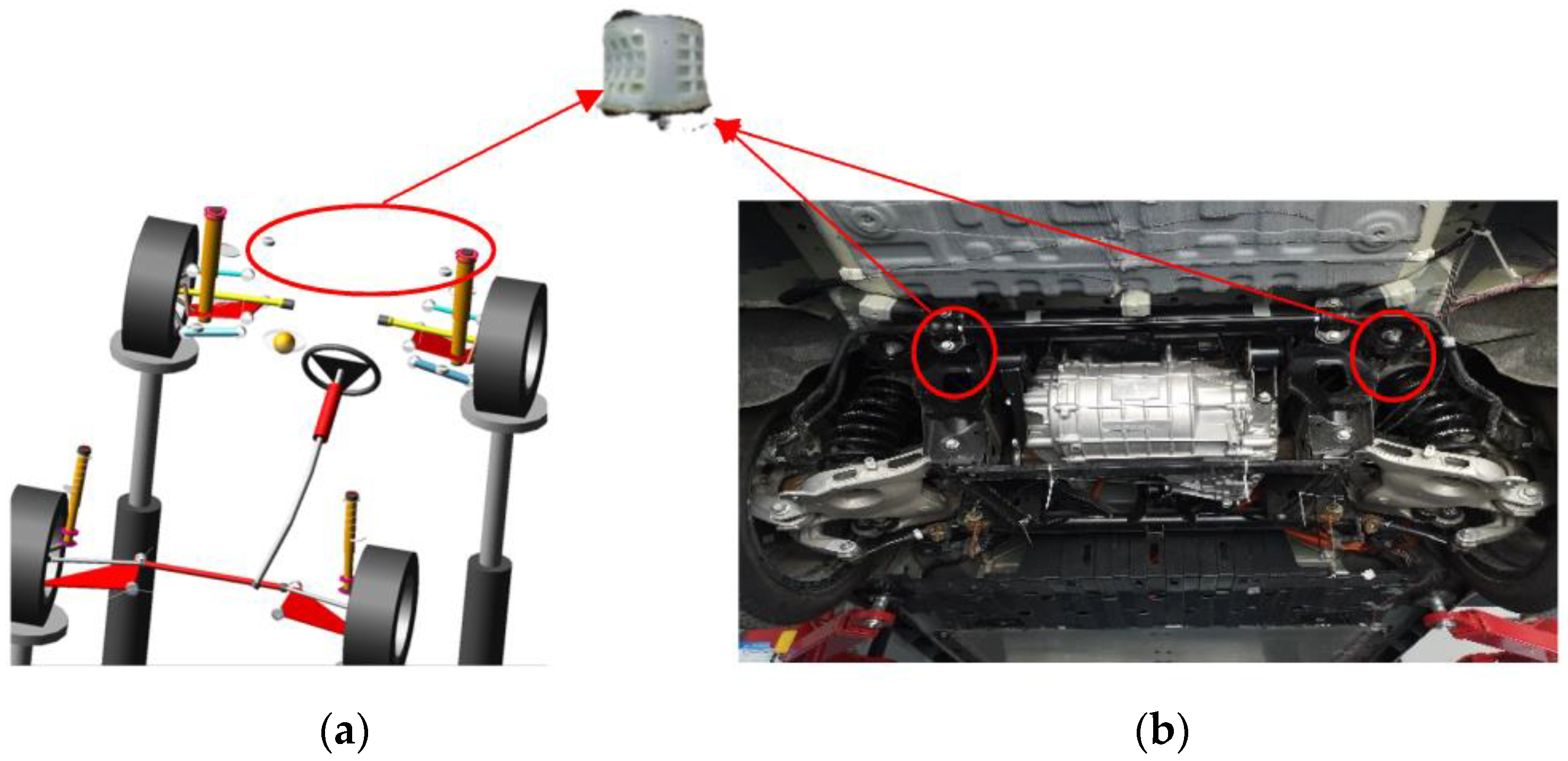
1. Introduction

The suspension and body of the pure electric vehicle are connected through rubber bushings on the subframe, which play a role in bearing multi-directional loads [1]. This can reduce the forces and impacts transmitted to the body from the road surface, improving the overall NVH performance of the vehicle [2]. The rubber in the subframe bushings exhibits strong nonlinear viscoelastic properties, which are greatly influenced by factors such as load amplitude, load frequency, and operating cycle. The accuracy of the rubber bushing model is one of the key factors affecting the precision of suspension and vehicle dynamic simulation, especially when considering the impact on suspension KC characteristics, vehicle handling stability, ride comfort, and other performance indicators.

Many scholars from both domestic and international backgrounds have proposed numerous dynamic models for bushings, with early models mainly based on linear viscoelastic models, such as the Kelvin–Voigt model, Zener model, and linear characteristic bushing model in ADAMS [3]. However, these traditional linear models fail to accurately describe the nonlinear hysteresis characteristics of rubber bushings. Therefore, it is necessary to consider establishing models that accurately reflect the dynamic nonlinear characteristics of the bushings. Domestic scholar Sun Beibei utilized a parallel combination of the Maxwell model, spring elements, and friction elements to simulate the dynamic behavior of rubber bushings [4]. Professor Stawomir Dzierzek from Cracow University of Technology proposed the Dzierzek model [5].

To describe the dynamic characteristics of rubber bushings more accurately, some scholars have found that fractional derivative models can be used to describe viscoelastic properties with few parameters; both domestic and international scholars, such as Metzler, Bagley, and Lin Song [6,7], have, respectively, employed fractional derivative models to study the viscoelastic properties of rubber bushings [8,9,10]. Some scholars have also combined fractional-order Maxwell and fractional-order Kelvin–Voigt models in series or parallel to obtain high-order fractional derivative models [11,12] and improved the overall prediction accuracy through related algorithms for parameter identification. They have identified model parameters using appropriate algorithms to improve overall prediction accuracy. Particle swarm and genetic algorithms are commonly employed for parameter identification when dealing with a large number of parameters [13].

In this paper, a rubber bushing in the rear sub-frame of a specific electric vehicle was taken as the object of study, and the test and modeling are mainly conducted in the radial solid direction, as shown in Figure 1a,b. The rubber bushing model is illustrated in Figure 2a,b.

The FVMS (fractional Voigt and Maxwell model in series) viscoelastic model was considered for establishing the dynamic model of the rubber bushing. The ACMPSO (adaptive chaos improved particle swarm optimization) algorithm was employed in conjunction with experimental data to fit the parameters of the rubber bushing model. Furthermore, to enhance the model accuracy, sensitivity analysis of the model parameters was conducted, and the parameters with high correlation coefficients were identified by incorporating test data under different amplitudes, aiming to reduce errors and improve the model precision.

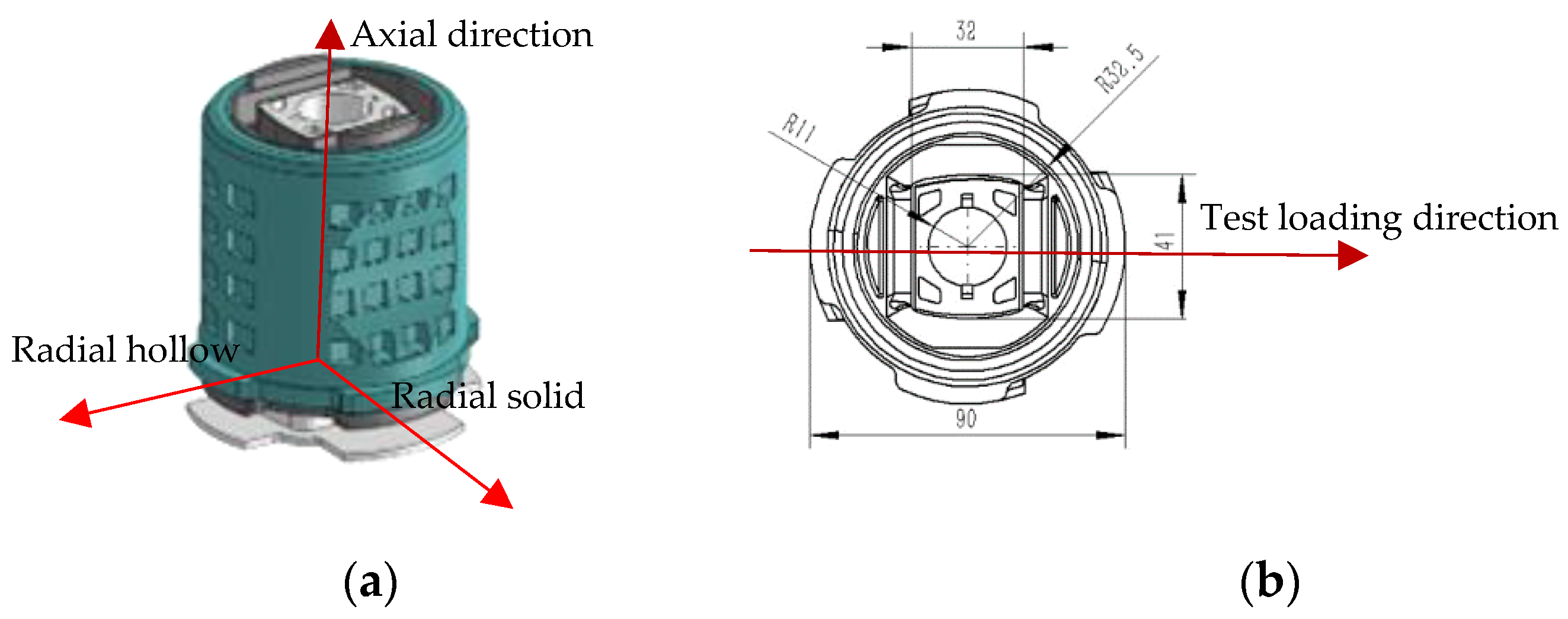
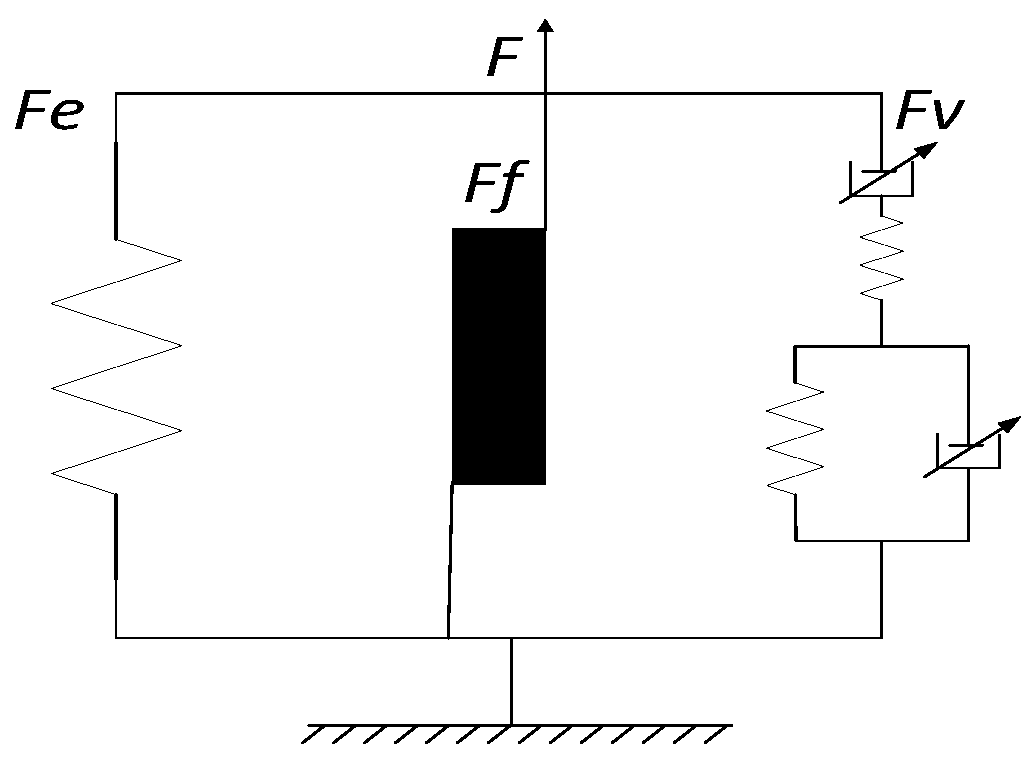
2. Establishment of the Rubber Bushing Dynamic Model

The dynamic model of the rubber bushing comprises three components: the elastic elements, friction hysteresis elements, and viscoelastic elements. These components are arranged in parallel, allowing for the expression of the overall force and moment characteristics by combining the forces from each element. The dynamic model of the bushing is visually represented in Figure 3.

The dynamic model of the rubber bushing was constructed with three elements in parallel: an elastic, a frictional, and a viscoelastic element. The forces of these three elements were superimposed to express the force and torque characteristics of the entire bushing model, as shown in Figure 3.

$$F=F_e+F_f+F_v$$

(1)

Equation (1) was used to calculate the response force of the whole parameterized model; $F_e$ represents the elastic force, $F_f$ represents the force of frictional hysteresis, and $F_v$ represents the force of viscoelastic (Units in Appendix A). $F$ denotes the response force of the entire parameterized model.

2.1. Elastic Element of the Rubber Bushing Model

The static characteristics of the bushing are caused by its elastic deformation. Constitutive models commonly used to describe the static mechanical behavior include the Mooney–Rivlin model [14], neo-Hookean model [15], Yeoh model [16], Ogden model [17], etc. The parameters in these models represent the physical meaning of the rubber bushing material properties and describe the relationship between stress and strain. Since this article considers the relationship between force and displacement, a nonlinear spring is used to represent the elastic element. The mechanical expression of this element can be described as [18]:

$$F_e=a_0+a_{1}x+a_{{}_2}{x}^2+\dots \dots +a_n{x}^n$$

(2)

The amplitude of the elastic module, denoted as $F_{e0}$, under the sinusoidal excitation with an amplitude of $x_0$ can be expressed as:

$$F_{e0}=a_0+a_1{x}_0+a_{{}_2}{x}_0{}^2+\dots \dots +a_n{x}_0{}^n$$

(3)

The elastic module does not consider friction, so there is no energy loss.

2.2. Frictional Element of the Rubber Bushing Model

Regarding the friction hysteresis module of the rubber bushing model, the hysteresis effect of the rubber bushing becomes more pronounced as the deformation from loading increases. A smooth friction force model is used to express this behavior, and the expression is as follows [19]:

$$F_f=\begin{array}{l}{F}_{fs}+\frac{\left(x-x_s\right)\left(F_{f\max }+F_{fs}\right)}{x_2\left(1+u\right)-\left(x-x_s\right)}\left(x<x_s\right)\\ F_{fs} \left(x=x_s\right)\\ F_{fs}+\frac{\left(x-x_s\right)\left(F_{f\max }+F_{fs}\right)}{x_2\left(1+u\right)+\left(x-x_s\right)}\left(x>x_s\right)\end{array}$$

(4)

In Equation (4), $F_f$ represents the friction force, $x$ represents the displacement unit of the loading, $F_{fmax}$ is the maximum friction force, $x_2$ is the displacement of the friction force from 0 to $F_{fmax}$/2, and ($x_s$, $F_{fs}$) is a reference point on the force–displacement curve obtained from static loading tests. Under sinusoidal excitation with amplitude $x_0$, the amplitude of the friction hysteresis module is given by:

$$F_{f0}=\frac{F_{fmax}}{2x_2}\left(\sqrt{x_0{}^2+x_2{}^2+6x_0{x}_2}-x_0-x_2\right)$$

(5)

$$E_f=2F_{fmax}\left[2x_0-x_2{(1+u)}^{2}ln\frac{x_2\left(1+u\right)+2x_0}{x_2\left(1+u\right)}\right]$$

(6)

In the Equation (6), $u$ =$F_{f0}/F_{fmax}$, $E_f$ represents the energy loss per cycle.

2.3. Viscoelastic Element of the Bushing Model

In the parameterized model of the bushing, the most common standard mechanical models for the viscoelastic module are the Kelvin–Voigt model and the Maxwell model. However, the standard mechanical models cannot accurately describe the viscoelasticity of the bushing. In order to better represent the viscoelastic characteristics of the bushing, the fraction Voigt model (FVM) and fraction Maxwell model (FMM) were proposed based on the Kelvin–Voigt model and Maxwell model, respectively. Furthermore, a FVMS model was developed by combining a Kelvin–Voigt fractional derivative model and a Maxwell fractional derivative model in series, creating a high–order fractional derivative model for describing the viscoelasticity of the rubber bushing. When the coefficients of fractional derivatives in the FVMS model are all 1, it is the Burgers model [20], so the FVMS model has stronger generalization ability than the Burgers model.

$${}_0{D}_t^{\beta +\gamma }x(\mathrm{t})k_2{+}_0{D}_t^{\beta }x(\mathrm{t}){\lambda }_1{k}_2{=}_0{D}_t^{\alpha +\gamma }{F}_v(\mathrm{t}){+}_0{D}_t^{\alpha }{F}_v(\mathrm{t}){\lambda }_1{+}_0{D}_t^{\beta }{F}_v(\mathrm{t})\frac{k_2}{c_1}{+}_0{D}_t^{\gamma }{F}_v(t){\lambda }_2+{\lambda }_1{\lambda }_2{F}_v(\mathrm{t})$$

(7)

In Equation (7), ₀$D_t^{\alpha }{F}_v\left(t\right)$ represents the α–order derivative of $F_v\left(t\right)$; $k_1, k_2, c_1, c_2$, respectively, are the elastic element and the viscosity coefficient of the viscoelastic element; $k_1, c_1$, respectively, are the elastic modulus and viscosity coefficient of FVM in viscoelastic element; $k_2, c_2$, respectively, are the elastic modulus and viscosity coefficient of FMM in viscoelastic element. ${\lambda }_1=k_1/c_1 , {\lambda }_2=k_2/c_2$ are defined, respectively. $F_v\left(t\right)$ represents the viscoelastic force, and $x\left(t\right)$ is the loading displacement. $\alpha , \beta , \gamma$ is the fractional derivative order, and its value range is (0, 1). To satisfy the thermodynamic stability condition, α ≤ β [11]; thus, the maximum order is $\beta +\gamma$, with the maximum value being 2. The Laplace transform of the Equation (7) is as follows:

$$(k_2{\mathrm{s}}^{\beta +\gamma }+{\lambda }_1{\mathrm{s}}^{\beta })\mathrm{x}(\mathrm{s})=[{\mathrm{s}}^{\alpha +\gamma }+{\lambda }_1{\mathrm{s}}^{\alpha }+\frac{k_2}{c_1}{\mathrm{s}}^{\beta }+{\lambda }_2{\mathrm{s}}^{\gamma }+{\lambda }_1{\lambda }_2]\mathrm{F}(\mathrm{s})$$

(8)

Then, the complex stiffness of the viscoelastic element is Equation (9):

$$K_v^{*}(\mathrm{s})=\frac{F(\mathrm{s})}{x(\mathrm{s})}=\frac{k_2{\mathrm{s}}^{\beta +\gamma }+{\lambda }_1{\mathrm{s}}^{\beta }}{{\mathrm{s}}^{\alpha +\gamma }+{\lambda }_1{\mathrm{s}}^{\alpha }+\frac{k_2}{c_1}{\mathrm{s}}^{\beta }+{\lambda }_2{\mathrm{s}}^{\gamma }+{\lambda }_1{\lambda }_2}$$

(9)

$k_v^{*}\left(\omega \right)$ is the complex stiffness of the viscoelastic element. By transforming Equation (9) into the frequency domain, we obtain the frequency domain expression of the fractional derivative model as follows:

$$K_v^{*}(\omega )=\frac{F(\omega )}{x(\omega )}=\frac{k_2{(\mathrm{i}\omega )}^{\beta +\gamma }+{\lambda }_1{(\mathrm{i}\omega )}^{\beta }}{{(\mathrm{i}\omega )}^{\alpha +\gamma }+{\lambda }_1{(\mathrm{i}\omega )}^{\alpha }+\frac{k_2}{c_1}{(\mathrm{i}\omega )}^{\beta }+{\lambda }_2{(\mathrm{i}\omega )}^{\gamma }+{\lambda }_1{\lambda }_2}$$

(10)

$${(\mathrm{i}\omega )}^{\alpha }={\omega }^{\alpha }{e}^{\mathrm{i}\pi \alpha /2+2n\pi \alpha }$$

(11)

Let n = 0, as the taproot, then:

$${(\mathrm{i}\omega )}^{\alpha }={\omega }^{\alpha }{e}^{i\pi \alpha /2}$$

(12)

It is obtained by Euler’s formula:

$${(\mathrm{i}\omega )}^{\alpha }={\omega }^{\alpha }(\mathrm{c}\mathrm{o}\mathrm{s}(\frac{\alpha \pi }{2})+\mathrm{i}\mathrm{s}\mathrm{i}\mathrm{n}(\frac{\alpha \pi }{2}))$$

(13)

Put Equation (13) into Equation (10):

$$K_v^{*}(\omega )=\frac{\left[\begin{array}{l}{k}_2{\lambda }_1{\omega }^{\alpha +\gamma +\beta }\cos \left(\frac{\alpha +\gamma -\beta }{2}\pi \right)+{\lambda }_1{k}_2{\omega }^{\alpha +\gamma +\beta }\cos \left(\frac{\beta +\gamma -\alpha }{2}\pi \right)+\frac{k_2^2}{c_1}{\omega }^{\gamma +2\beta }\cos \left(\frac{\gamma }{2}\pi \right)+\frac{k_2^2}{c_1}{\lambda }_1{\omega }^{2\beta }+k_2{\lambda }_2{\lambda }_1{\omega }^{\gamma +\beta }\cos \left(\frac{\beta -\gamma }{2}\pi \right)+k_2{\lambda }_2{\lambda }_1{\omega }^{\gamma +\beta }\cos \left(\frac{\beta +\gamma }{2}\pi \right)+\left(k_2{\omega }^{\alpha +\beta +2\gamma }+k_2{\lambda }_1^2{\omega }^{2\beta +\gamma }\right)\cos \left(\frac{\beta -\alpha }{2}\pi \right)+\\ \left(k_2{\lambda }_2{\omega }^{\beta +2\gamma }+{\lambda }_1^2{k}_2{\lambda }_2{\omega }^{\beta }\right)\cos \left(\frac{\beta }{2}\pi \right)+k_2{\lambda }_1{\omega }^{\alpha +\gamma +\beta }\sin \left(\frac{\alpha +\gamma -\beta }{2}\pi \right)i+{\lambda }_1{k}_2{\omega }^{\alpha +\gamma +\beta }\sin \left(\frac{\beta +\gamma -\alpha }{2}\pi \right)i+k_2{\lambda }_2{\lambda }_1{\omega }^{\gamma +\beta }\sin \left(\frac{\beta -\gamma }{2}\pi \right)i+k_2{\lambda }_2{\lambda }_1{\omega }^{\gamma +\beta }\sin \left(\frac{\beta +\gamma }{2}\pi \right)i+\left(k_2{\omega }^{\alpha +\beta +2\gamma }+k_2{\lambda }_1^2{\omega }^{2\beta +\gamma }\right)\sin \left(\frac{\beta -\alpha }{2}\pi \right)i+\\ \left(k_2{\lambda }_2{\omega }^{\beta +2\gamma }+{\lambda }_1^2{k}_2{\lambda }_2{\omega }^{\beta }\right)\sin \left(\frac{\beta }{2}\pi \right)i+\frac{k_2^2}{c_1}{\omega }^{\gamma +2\beta }\sin \left(\frac{\gamma }{2}\pi \right)i\end{array}\right]}{\left[\begin{array}{l}{\omega }^{2\left(\alpha +\gamma \right)}+{\lambda }_1^2{\omega }^{2\alpha }+\frac{k_2^2}{c_1^2}{\omega }^{2\beta }+c_1^2{c}_2^2+c_2^2{\omega }^{2\gamma }+2\frac{k_2}{c_1}{\omega }^{\alpha +\beta +\gamma }\cos \left(\frac{\alpha +\gamma -\beta }{2}\pi \right)+2\frac{{\lambda }_1{k}_2}{c_1}{\omega }^{\alpha +\beta }\cos \left(\frac{\alpha -\beta }{2}\pi \right)+2c_1{c}_2{\omega }^{\alpha +\gamma }\cos \left(\frac{\alpha -\gamma }{2}\pi \right)+2\frac{k_2{\lambda }_2}{c_1}{\omega }^{\beta +\gamma }\cos \left(\frac{\beta -\gamma }{2}\pi \right)+\\ 2c_1{c}_2{\omega }^{\alpha +\gamma }\cos \left(\frac{\alpha -\gamma }{2}\pi \right)+2\frac{k2}{c1}{\lambda }_1{\lambda }_2{\omega }^{\beta }\cos \left(\frac{\beta \pi }{2}\right)+\left(2{\lambda }_1{\omega }^{2\alpha +\gamma }+2{\lambda }_1{\lambda }_2^2{\omega }^{\gamma }\right)\cos \left(\frac{\gamma \pi }{2}\right)+\left(2{\lambda }_2{\omega }^{\alpha +2\gamma }+2{\lambda }_2{\lambda }_1^2{\omega }^{\alpha }\right)\cos \left(\frac{\alpha \pi }{2}\right)\end{array}\right]}$$

(14)

Based on the above formula, it is further deduced that under the sinusoidal excitation of the amplitude $x_0$, the amplitudes $F_{v0\mathrm{Re}}$ and $F_{v0lm}$ of the real and imaginary parts of the response force are, respectively:

$$\begin{gathered} F_{v0\mathrm{Re}}=\frac{\left[\begin{array}{l}{k}_2{\lambda }_1{\omega }^{\alpha +\gamma +\beta }\cos \left(\frac{\alpha +\gamma -\beta }{2}\pi \right)+{\lambda }_1{k}_2{\omega }^{\alpha +\gamma +\beta }\cos \left(\frac{\beta +\gamma -\alpha }{2}\pi \right)+\frac{k_2^2}{c_1}{\omega }^{\gamma +2\beta }\cos \left(\frac{\gamma }{2}\pi \right)+\frac{k_2^2}{c_1}{\lambda }_1{\omega }^{2\beta }+k_2{\lambda }_2{\lambda }_1{\omega }^{\gamma +\beta }\cos \left(\frac{\beta -\gamma }{2}\pi \right)+k_2{\lambda }_2{\lambda }_1{\omega }^{\gamma +\beta }\cos \left(\frac{\beta +\gamma }{2}\pi \right)+\\ \left(k_2{\omega }^{\alpha +\beta +2\gamma }+k_2{\lambda }_1^2{\omega }^{2\beta +\gamma }\right)\cos \left(\frac{\beta -\alpha }{2}\pi \right)+\left(k_2{\lambda }_2{\omega }^{\beta +2\gamma }+{\lambda }_1^2{k}_2{\lambda }_2{\omega }^{\beta }\right)\cos \left(\frac{\beta }{2}\pi \right)\end{array}\right]}{\left[\begin{array}{l}{\omega }^{2\left(\alpha +\gamma \right)}+{\lambda }_1^2{\omega }^{2\alpha }+\frac{k_2^2}{c_1^2}{\omega }^{2\beta }+c_1^2{c}_2^2+c_2^2{\omega }^{2\gamma }+2\frac{k_2}{c_1}{\omega }^{\alpha +\beta +\gamma }\cos \left(\frac{\alpha +\gamma -\beta }{2}\pi \right)+2\frac{{\lambda }_1{k}_2}{c_1}{\omega }^{\alpha +\beta }\cos \left(\frac{\alpha -\beta }{2}\pi \right)+2c_1{c}_2{\omega }^{\alpha +\gamma }\cos \left(\frac{\alpha -\gamma }{2}\pi \right)+2\frac{k_2{\lambda }_2}{c_1}{\omega }^{\beta +\gamma }\cos \left(\frac{\beta -\gamma }{2}\pi \right)+\\ 2c_1{c}_2{\omega }^{\alpha +\gamma }\cos \left(\frac{\alpha -\gamma }{2}\pi \right)+2\frac{k2}{c1}{\lambda }_1{\lambda }_2{\omega }^{\beta }\cos \left(\frac{\beta \pi }{2}\right)+\left(2{\lambda }_1{\omega }^{2\alpha +\gamma }+2{\lambda }_1{\lambda }_2^2{\omega }^{\gamma }\right)\cos \left(\frac{\gamma \pi }{2}\right)+\left(2{\lambda }_2{\omega }^{\alpha +2\gamma }+2{\lambda }_2{\lambda }_1^2{\omega }^{\alpha }\right)\cos \left(\frac{\alpha \pi }{2}\right)\end{array}\right]}{x}_0 \\ {F}_{v0lm}=\frac{\left[\begin{array}{l}{k}_2{\lambda }_1{\omega }^{\alpha +\gamma +\beta }\sin \left(\frac{\alpha +\gamma -\beta }{2}\pi \right)+{\lambda }_1{k}_2{\omega }^{\alpha +\gamma +\beta }\sin \left(\frac{\beta +\gamma -\alpha }{2}\pi \right)+k_2{\lambda }_2{\lambda }_1{\omega }^{\gamma +\beta }\sin \left(\frac{\beta -\gamma }{2}\pi \right)+k_2{\lambda }_2{\lambda }_1{\omega }^{\gamma +\beta }\sin \left(\frac{\beta +\gamma }{2}\pi \right)+\\ \left(k_2{\omega }^{\alpha +\beta +2\gamma }+k_2{\lambda }_1^2{\omega }^{2\beta +\gamma }\right)\sin \left(\frac{\beta -\alpha }{2}\pi \right)+\frac{k_2^2}{c_1}{\omega }^{\gamma +2\beta }\sin \left(\frac{\gamma }{2}\pi \right)\left(k_2{\lambda }_2{\omega }^{\beta +2\gamma }+{\lambda }_1^2{k}_2{\lambda }_2{\omega }^{\beta }\right)\sin \left(\frac{\beta }{2}\pi \right)\end{array}\right]}{\left[\begin{array}{l}{\omega }^{2\left(\alpha +\gamma \right)}+{\lambda }_1^2{\omega }^{2\alpha }+\frac{k_2^2}{c_1^2}{\omega }^{2\beta }+c_1^2{c}_2^2+c_2^2{\omega }^{2\gamma }+2\frac{k_2}{c_1}{\omega }^{\alpha +\beta +\gamma }\cos \left(\frac{\alpha +\gamma -\beta }{2}\pi \right)+2\frac{{\lambda }_1{k}_2}{c_1}{\omega }^{\alpha +\beta }\cos \left(\frac{\alpha -\beta }{2}\pi \right)+2c_1{c}_2{\omega }^{\alpha +\gamma }\cos \left(\frac{\alpha -\gamma }{2}\pi \right)+2\frac{k_2{\lambda }_2}{c_1}{\omega }^{\beta +\gamma }\cos \left(\frac{\beta -\gamma }{2}\pi \right)+\\ 2c_1{c}_2{\omega }^{\alpha +\gamma }\cos \left(\frac{\alpha -\gamma }{2}\pi \right)+2\frac{k2}{c1}{\lambda }_1{\lambda }_2{\omega }^{\beta }\cos \left(\frac{\beta \pi }{2}\right)+\left(2{\lambda }_1{\omega }^{2\alpha +\gamma }+2{\lambda }_1{\lambda }_2^2{\omega }^{\gamma }\right)\cos \left(\frac{\gamma \pi }{2}\right)+\left(2{\lambda }_2{\omega }^{\alpha +2\gamma }+2{\lambda }_2{\lambda }_1^2{\omega }^{\alpha }\right)\cos \left(\frac{\alpha \pi }{2}\right)\end{array}\right]}{x}_0 \end{gathered}$$

(15)

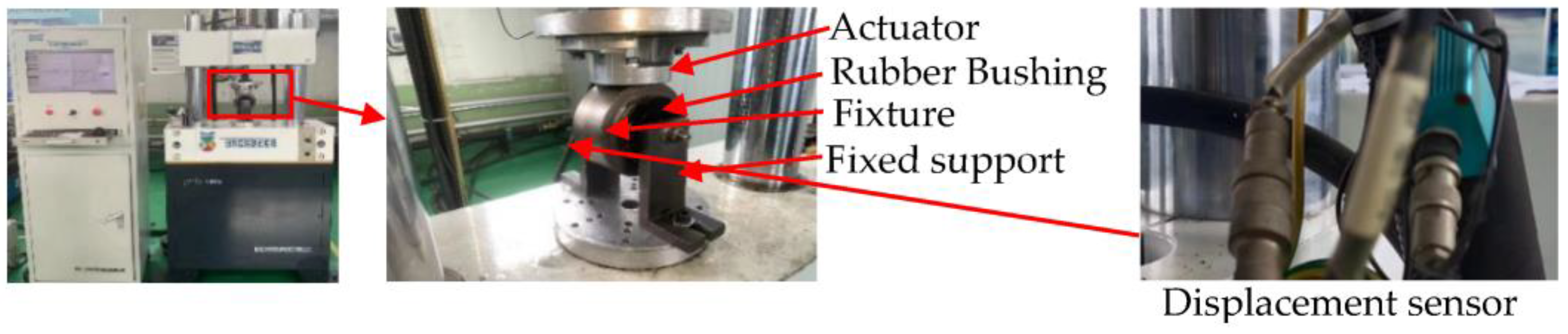
3. Rubber Bushing Tests

The quasi-static loading tests on the rubber bushing primarily aimed to investigate its mechanical response characteristics under slow loading conditions, providing essential raw data for static parameter identification.

During these tests, the rubber bushing was subjected to gradual and controlled loading, allowing researchers to observe and measure its deformation and corresponding reaction forces. The loading rate was carefully controlled to ensure a quasi-static condition, avoiding rapid or dynamic loading.

In addition to the quasi-static loading tests, wideband sinusoidal sweep tests were also conducted on the subject of this study, which is the rear sub–frame rubber bushing.

The wideband sinusoidal sweep test involves applying a sinusoidal excitation signal to the bushing over a range of frequencies. The excitation signal varies in frequency and amplitude, covering a broad frequency spectrum. This type of test is also known as frequency response analysis.

During the wideband sinusoidal sweep test, the bushing’s dynamic response was measured, including its frequency-dependent stiffness, damping, and resonance characteristics. This test provides valuable information about how the bushing behaves under different dynamic loading conditions and how it responds to vibrations across a range of frequencies.

The tests were performed using the LETRY Dynamic Stiffness Testing Platform, and it involved applying a sinusoidal signal with a specific amplitude to excite the bushing. The test setup is depicted in Figure 4.

To thoroughly investigate the dynamic characteristics of the rubber bushing and obtain sufficient raw data for parameter identification of the bushing model, dynamic loading tests were conducted at frequencies ranging from 1 to 41 Hz and with amplitudes of 0.2 mm, 0.3 mm, 0.5 mm, and 1 mm, respectively. The relationship curve between the dynamic stiffness of the rubber bushing and the loading frequency is shown in Figure 5.

From Figure 5, it can be observed that, at a certain frequency, the dynamic stiffness of the bushing decreases as the excitation amplitude increases. In the frequency range of 1 to 41 Hz with constant excitation amplitude, the dynamic stiffness of the bushing increases as the frequency increases.

4. Parameter Identification of the Rubber Bushing Dynamic Model

The parameter identification of the rubber bushing dynamic model involves two steps. Firstly, the identification of the parameters of the elastic element and the friction element, and then the identification of the parameters of the viscoelastic element.

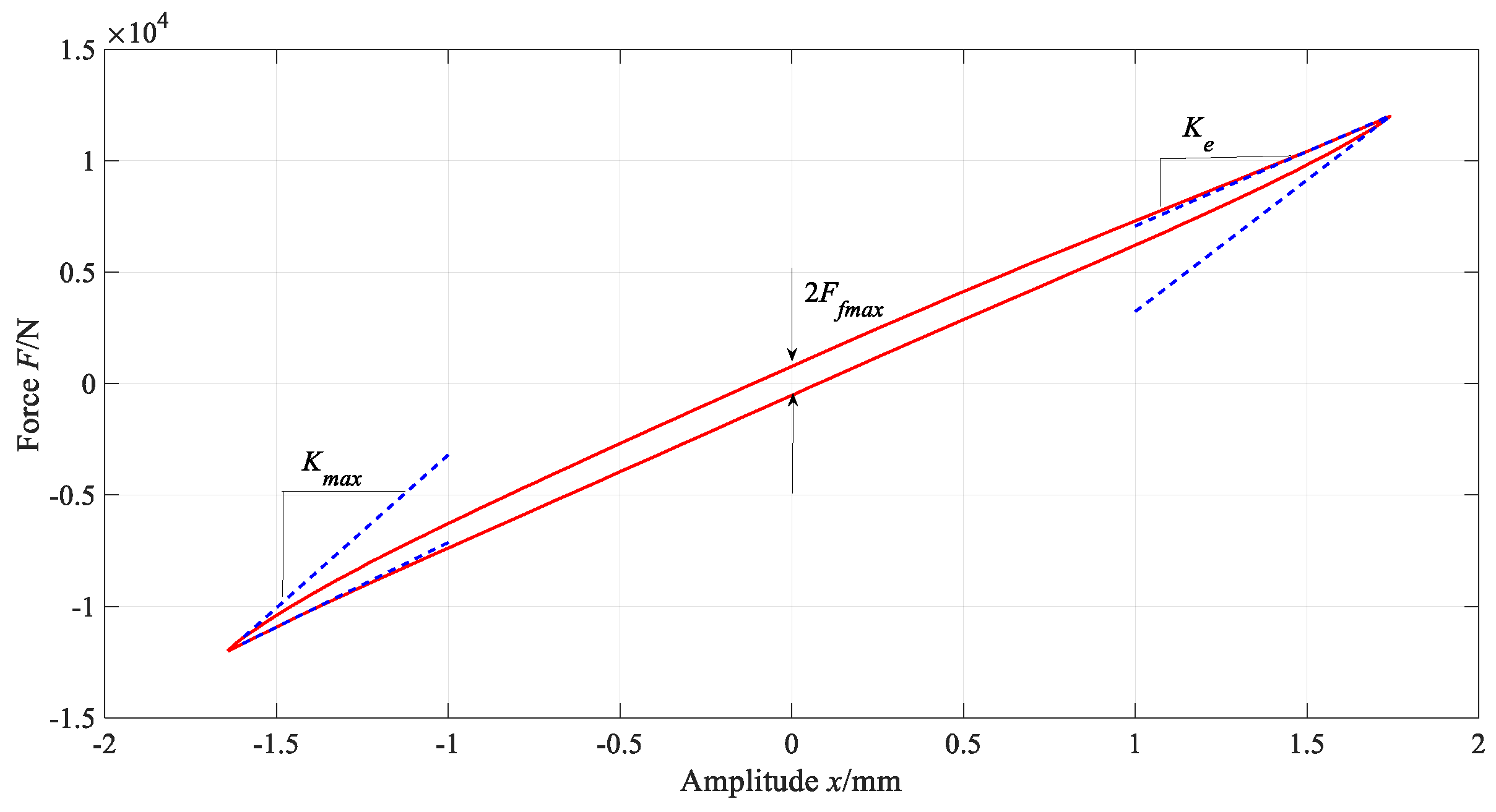
4.1. Identification of the Parameters of the Elastic and Friction Elements

The parameter identification process involves using the static loading test data, as shown in Figure 6. The slope of the curve near the limit position of displacement can be approximated to represent the static elastic stiffness $k_e$ of the bushing’s elastic unit. The maximum friction force $F_{fmax}$ in the friction model is obtained by taking half of the vertical distance between the upper and lower limits of the hysteresis loop. The maximum slope of the curve is denoted as $k_{max}$, and by using Equation (16), the displacement $x_2$ in the friction unit can be determined.

$$x_2=F_{f\max }/(k_{max}-k_e)$$

(16)

The upper and lower boundary curves of the hysteresis curve in Figure 6 were overlaid by shifting, obtaining the force–displacement test curve of the elastic element. The data of this curve were fitted using a third–order polynomial spring model, as shown in Figure 7. Results of parameter identification for the elastic and friction elements are shown in

Table 1. Results of elastic and friction unit parameter identification for the rubber bushing model.

Model Element	Parameter	Result
Elastic elements	${\mathrm{k}}_e$/($\mathrm{N}\cdot {\mathrm{mm}}^{-1}$)	6663.68
	$n$	3
	$a_3$	85.12
	$a_2$	−187.2
	$a_1$	6782
	$a_0$	136.2
Friction elements	${\mathrm{k}}_{\max }$/($\mathrm{N}\cdot {\mathrm{mm}}^{-1}$)	11,814.9
	$F_{f\max }$/$\mathrm{N}$	647.6625
	$x_2$/($\mathrm{mm}$)	0.1257

.

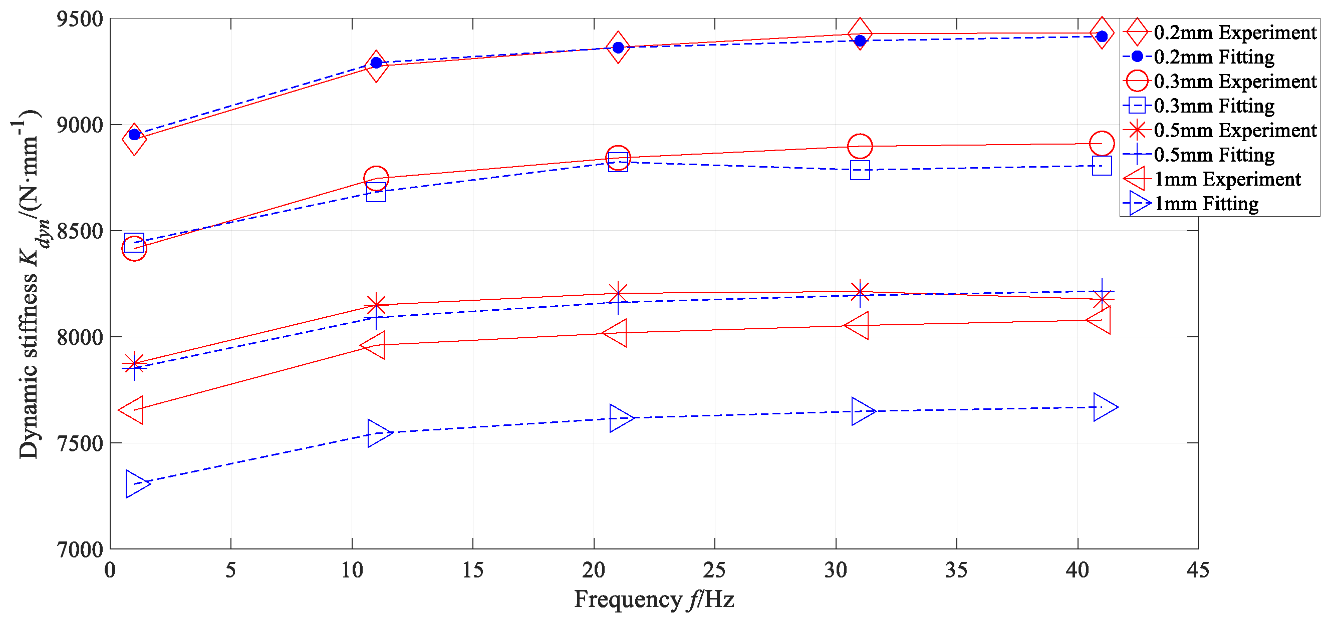
4.2. Identification of the Parameters of the Viscoelastic Elements

The identification of parameters for the rubber bushing’s viscoelastic elements was conducted using dynamic loading test curves. Due to the numerous parameters that need to be identified and the strong nonlinearity of the viscoelastic unit, the particle swarm optimization (PSO) algorithm was employed to search for the optimal solution based on fitness evaluation. The PSO algorithm updates the fitness, velocity, and position of particles iteratively to find the best parameters. The corresponding Equation (17) is as follows:

$$\begin{array}{l}{v}_{t+1}=w{v}_t+c_1{r}_1({\mathrm{p}}_b-x_t)+{\mathrm{c}}_2{r}_2({\mathrm{g}}_b-x_t)\\ x_{t+1}=x_t+v_{t+1}\end{array}$$

(17)

where $w$ is the inertia weight; the velocity and position of the current particle are represented by $v_t$ and $x_t$; $r_1$ and $r_2$ are random numbers ranging between 0 and 1; $c_1$ and $c_2$ are learning factors; the range of the velocity and position of the particles are [$v_{min}, v_{max}$] and [$x_{min}, x_{max}$], respectively; $p_b$ is the best position (parameter values) of particle i found so far in the iterations; ${\mathrm{g}}_b$ is the best position among all particles in the swarm at iteration t.

To improve the optimization speed, a modification has been made in the particle swarm optimization (PSO) algorithm, where a random particle is selected to update the velocity during the velocity update process. This approach, known as “random particle updating”, helps accelerate the optimization process and prevents the algorithm from getting stuck in local optima. The velocity update formula with random particle updating is given by Equation (18).

$$\begin{array}{l}{v}_{t+1}=w{v}_t+c_1{r}_1({\mathrm{p}}_b-x_t)+{\mathrm{c}}_2{r}_2({\mathrm{g}}_b-x_t)\\ +c_3{r}_3({\mathrm{p}}_s-x_t)\end{array}$$

(18)

$c_3$ is an additional coefficient introduced for the random particle updating, controlling the influence of the random particle’s position on the velocity update; $r_3$ is a random number ranging between 0 and 1; $p_s$ is the randomly selected particle from the current particle swarm.

To evaluate the results of each optimization, this study uses an optimization degree λ to assess the effectiveness of the search process. The optimization degree, denoted as “OD”, is a measure of how much the global fitness changes during the search. If the global fitness changes during the current search, the optimization degree is set to 1. However, if the global fitness remains unchanged during the current search, the optimization degree is calculated using the following Equation (19):

$$\lambda =\frac{\left|f_{mp}(\mathrm{i})-f_{best}\right|+1}{\left|f_{mp}(\mathrm{i}-1)-f_{best}\right|+1}$$

(19)

where $f_{mp}\left(i\right)$ is the average fitness value of the i-th optimization search population, and $f_{best}\left(i\right)$ is the best fitness value of the current population.

A larger inertia weight $w$ is advantageous for global search, while a smaller inertia weight is advantageous for local search. By adjusting the inertia weight in a timely manner based on the optimization degree $\lambda$ of each optimization search, it is possible to search for the best particle [21].

$$\begin{gathered} w=w_{\max }-(w_{\max }-w_{\min })\times \sqrt{\frac{i}{G}}+(\ast ) \\ (\ast )=\left\{\begin{array}{l}\frac{\lambda -1}{D}, \lambda \ne 1\\ 0, \lambda =1\end{array}\right. \end{gathered}$$

(20)

Equation (20) is used to update the inertia weight; D represents the population size of the particles, and G represents the maximum number of iterations.

The parameter identification of the rubber bushing model’s viscoelastic element is essentially an optimal parameter estimation problem. To ensure that the identified parameters closely match the experimental data, an appropriate fitness function needs to be established. This is achieved by setting up an optimization function that minimizes the error between the numerical and experimental values based on the designed parameterized dynamic model. The objective function, based on the errors in dynamic stiffness, is formulated as follows in Equation (21):

$$F_{obj}={\displaystyle \sum _{i=1}^n\left[{\left(\frac{k_{dyn}^i-k_{dyn\_t}^i}{k_{dyn\_t}^i}\right)}^2\right]}$$

(21)

where n is the number of identification conditions, $k_{dyn\_t}^i$ represents the dynamic stiffness test data, and $k_{dyn}^i$ represents the dynamic stiffness of the i-th condition calculated by the bushing dynamics model.

To ensure the accuracy of parameter identification for the rubber bushing model and improve the fitting precision of the model, it is important to enforce constraints during the parameter identification process to prevent significant discrepancies between the model’s fitted data and the experimental data. Therefore, the following constraints are established:

$$\left|\frac{k_{dyn}^i-k_{dyn\_t}^i}{k_{dyn\_t}^i}\right|\le 0.1$$

(22)

Calculate the bushing dynamic stiffness using Equation (23):

$$\begin{gathered} F_0=\sqrt{{(F_{e0}+F_{f0}+F_{v0\mathrm{Re}})}^2+(F_{v0\mathrm{lm}}{}^2)} \\ {K}_{dyn}=\raisebox{1ex}{$F_0$}\!\left/ \!\raisebox{-1ex}{$x_0$}\right. \end{gathered}$$

(23)

The objective function Equation (21) is used as the fitness function for the parameter identification of the rubber bushing model. Two different optimization algorithms, adaptive chaotic multi-particle swarm optimization (ACMPSO) and particle swarm optimization (PSO), are applied to identify the parameters of the viscoelastic element.

After debugging, the following algorithm parameters are selected:

Population size: 50, particle dimension: 7, position vector $x=\left(k_1,k_2,c_1,c_2,\alpha ,\beta ,\gamma \right)$, particle search space lower limit $x_{min}=\left(0,0,0,0,0,0,0\right)$, particle search space upper limit $x_{min}=\left(500,500,500,500,1,1,1\right)$, maximum inertia weight $w_{max}=1.2$, minimum inertia weight $w_{min}=0.1$, learning factors $c_1=1.5$, $c_2=1.5$, $c_3=0.5$, and maximum number of iterations of 300. The PSO algorithm uses linearly decreasing inertia weight. The identification process is carried out using 0.2 mm dynamic stiffness data, as shown in Figure 8.

Figure 9 is a comparison of the optimization performance between the two algorithms, and it is clear that the PSO algorithm has fallen into premature convergence, while the ACMPSO algorithm has a stronger optimization ability.

Figure 10 illustrates the results of parameter identification and model fitting based on the rubber bushing dynamic model using experimental data obtained from a 0.2 mm amplitude test. The model is then used to fit dynamic stiffness data obtained from tests with amplitudes of 0.2 mm, 0.3 mm, 0.5 mm, and 1 mm, respectively.

As shown in Figure 11, the dynamic model’s fitted data for bushing amplitudes of 0.2 mm, 0.3 mm, and 0.5 mm closely match the test data with little deviation. However, when comparing the fitted data with the experimental data for the large amplitude of 1 mm loading test condition, it is evident that the fitting accuracy has decreased. The identification parameter results are shown in

Table 2. Identification results of bushing model parameters.

Model Parameter	Identification Results
$k_1/\left(N·s^{\beta -\gamma }\right)$	1.2766
$k_2/\left(N·s^{\beta -\mathsf{\alpha }}\right)$	243.8196
$c_1/\left(N·s^{\gamma }\right)$	49.2227
$c_2/\left(N·s^{\beta }\right)$	15.2644
$\alpha$	0.8913
$\beta$	0.9863
$\gamma$	0.937

.

5. Parameter Sensitivity Analysis of Viscoelastic Element of the Rubber Bushing Model

5.1. Choice of Parameter Sensitivity Analysis Method

Parameter sensitivity analysis is an empirical analysis method used to evaluate the sensitivity of a model’s output results to variations in its input parameters. Commonly used methods for parameter sensitivity analysis include one-factor-at-a-time analysis, the Morris method, and the Sobol method, among others.

Compared to other parameter sensitivity analysis methods, the Sobol method does not require individually varying each parameter. Instead, it estimates sensitivity indices using a set of randomly sampled parameter values, which significantly reduces the number of model simulations required. This advantage makes the Sobol method more widely applicable in cases with multiple parameters, especially in high-dimensional parameter spaces that involve extensive computations.

In this study, the parameter sensitivity analysis of the rubber bushing in the vehicle’s subframe is conducted using the Sobol method.

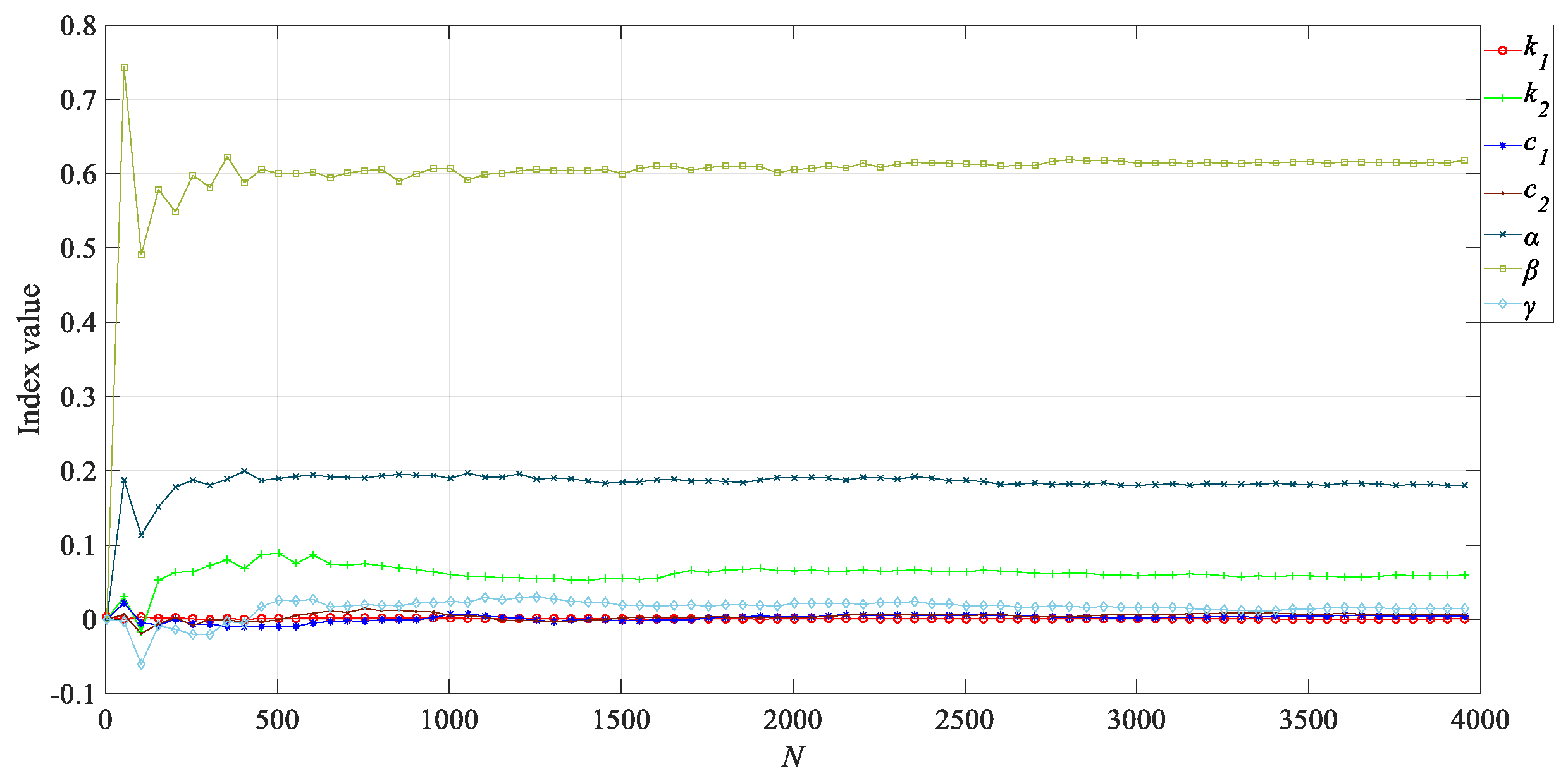
5.2. Sensitivity Analysis of Rubber Bushing Model Parameters Based on the Sobol Method

The Sobol method is a variance-based sensitivity analysis method that decomposes the variance of the target model output to quantify the influence of individual input parameters or combinations of parameters and their interactions. The method separates the effects of single parameters from the effects of combinations of parameters in multi-parameter set functions [22].

Any model can be regarded as $Y=f\left(x\right)$, where $f\left(x\right)$ can be decomposed according to Equation (24).

$$Y=f_0+{\displaystyle \sum _{i=1}^d{f}_i(X_i)+{\displaystyle \sum _{i<j}^d{f}_{ij}(X_i,X_j)+\cdots +f_{1,2,\cdots d}(X_1,X_2\cdots X_d)}}$$

(24)

$k=i_1, i_2\cdots i_s$. All terms in the decomposition are orthogonal. The definition of the conditional expectation of the function decomposition is given by Equation (25).

$$\left\{\begin{array}{l}{f}_0=E(Y)\\ f_i(X_i)=E(Y|X_j)-f_0\\ f_{ij}(X_i,X_j)=E(V|X_i,X_j)-f_0-f_i-f_j\end{array}\right.$$

(25)

Assuming further that $f\left(x\right)$ is square-integrable, the function can be squared and integrated after decomposition and expressed in the form of variance as:

$$V_{ar}(Y)={\displaystyle \sum _{i=1}^d{V}_i+}{\displaystyle \sum _{i<j}^d{V}_{ij}+\cdots +V_{1,2\cdots d}}$$

(26)

$$\left\{\begin{array}{l}{V}_i=V_{ar{X}_i}(E_{x_{-i}}(Y|X_i))\\ V_{ij}=V_{ar{X}_{ij}}(E_{x_{-ij}}(Y|X_i,X_j))-V_i-V_j\end{array}\right.$$

(27)

The sensitivity of each input is usually represented by a numerical value, called a sensitivity index.

The expression for the first-order Sobol’s index is given by Equation (28).

$$S_i=\frac{V_i}{V_{ar}(Y)}$$

(28)

The expression for the total-order Sobol’s index is given by Equation (29).

$$S_{Ti}=\frac{E_{X_{~i}}(V_{ar{X}_i}(Y|X_{~i}))}{V_{ar}(Y)}=1-\frac{V_{ar{x}_{~i}}(E_{x_i}(Y|X_{~i}))}{V_{ar}(Y)}$$

(29)

Using Monte Carlo estimation to calculate the above two indices, the expressions are as follows, where A and B are sample matrices.

$$V_i\approx \frac{1}{N}{\displaystyle \sum _N^{j=1}f{(B)}_j\left(f{(A_B^i)}_j-f{(A)}_j\right)}$$

(30)

$$E_{X_{~i}}(V_{ar{X}_i}(Y|X_{~i}))\approx \frac{1}{2N}{\displaystyle \sum _N^{j=1}{\left(f{(A_B^i)}_j-f{(A)}_j\right)}^2}$$

(31)

The Sobol method involves several steps, including the use of Monte Carlo estimation. Here are the main steps of the Sobol method:

• Set parameter ranges: Define the ranges of the input parameters for the model.
• Set the number of sampling points: In this study, the number of sampling points N ranges from 4 to 4000, increasing by 50 at each step.
• Monte Carlo sampling: Use the Monte Carlo method to randomly sample the input parameters within their specified ranges.
• Form the sample matrices A and B: Based on the Monte Carlo sampling, form the sample matrices A and B, which represent the input parameter values.
• Calculate the model output: Use the sample matrices A and B to calculate the model output for each set of input parameter values.
• Compute the first-order and total sensitivity indices: Utilize the model output to calculate the first-order sensitivity indices and total sensitivity indices for each input parameter. These indices measure the contribution of each parameter to the output variance and the total effect of each parameter, respectively.

By following these steps and gradually increasing the number of sampling points, the Sobol method allows for the evaluation of the sensitivity of the model to variations in the input parameters and helps to understand the relative importance of each parameter in influencing the model output.

Using the initial value range of the bushing model parameters in

Table 3. The initial value range of the bushing model parameters.

Model Parameter	Identification Results
$k_1/\left(N·s^{\beta -\gamma }\right)$	[0, 10]
$k_2/\left(N·s^{\beta -\mathsf{\alpha }}\right)$	[125, 400]
$c_1/\left(N·s^{\gamma }\right)$	[25, 75]
$c_2/\left(N·s^{\beta }\right)$	[10, 20]
$\alpha$	[0.5, 1]
$\beta$	[0.5, 1]
$\gamma$	[0.5, 1]

, the first-order Sobol sensitivity index and total effect index are calculated according to the analysis steps 1–6. The results are shown in Figure 12 and Figure 13 and

Table 4. First–order and total–order Sobol’s index of input parameters of bushing model.

Model Parameter	First–Order Sobol’s Index	Total–Order Sobol’s Index
$k_1/\left(N·s^{\beta -\gamma }\right)$	0.0007	0.0005
$k_2/\left(N·s^{\beta -\mathsf{\alpha }}\right)$	0.0593	0.1044
$c_1/\left(N·s^{\gamma }\right)$	0.0042	0.0145
$c_2/\left(N·s^{\beta }\right)$	0.0066	0.0220
$\alpha$	0.1807	0.2670
$\beta$	0.6180	0.7209
$\gamma$	0.0144	0.0388

.

As shown in Table 4, it was evident that the parameters $\alpha$, $\beta$, and $k_2$ had a significant impact on the dynamic stiffness prediction of the rubber bushing model. Therefore, these three parameters were subjected to parameter recalibration. Specifically, the dynamic characterization of the rubber bushing model’s parameters was re−identified using experimental data at 0.3 mm, 0.5 mm, and 1 mm amplitudes.

By comparing Figure 14 with Figure 15, it is found that the bushing model after parameter correction can better fit the test data. The error comparison before and after parameter correction is shown in

Table 5. Error comparison before and after the bushing model parameter correction.

Amplitude (mm)	Error before Correction (%)	Error before Correction (%)
0.3	4.07	2.43
0.5	4.42	4.38
1	28.82	7.45

.

6. Conclusions

This paper focuses on the dynamic analysis of the rubber bushing in the rear sub-frame of an electric vehicle. Based on dynamic loading frequency and amplitude-related experimental results, a rubber bushing dynamic model is established, comprising elastic, frictional, and viscoelastic elements. The following conclusions are drawn after conducting parameter identification and sensitivity analysis for the viscoelastic element of the bushing model:

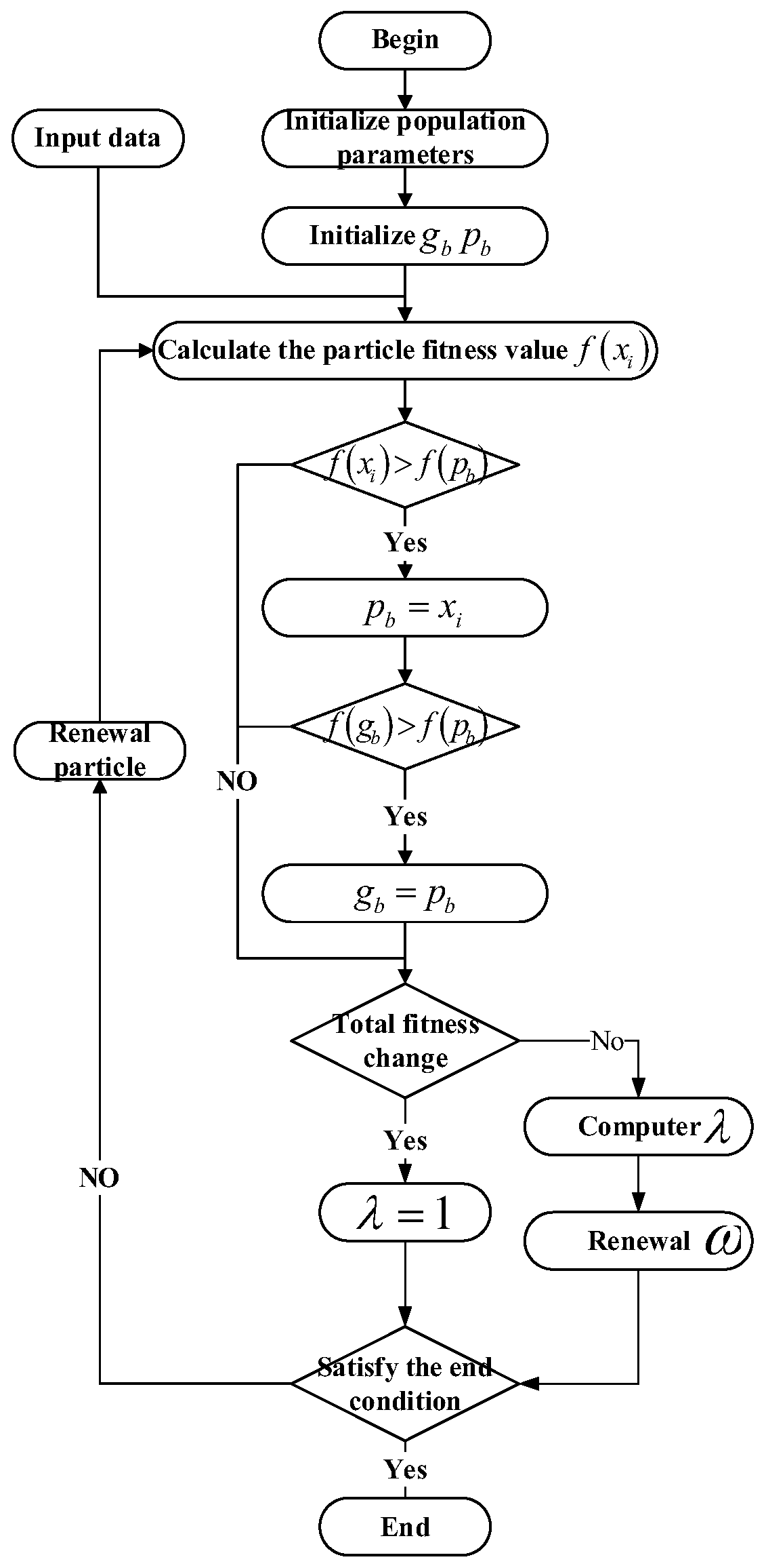
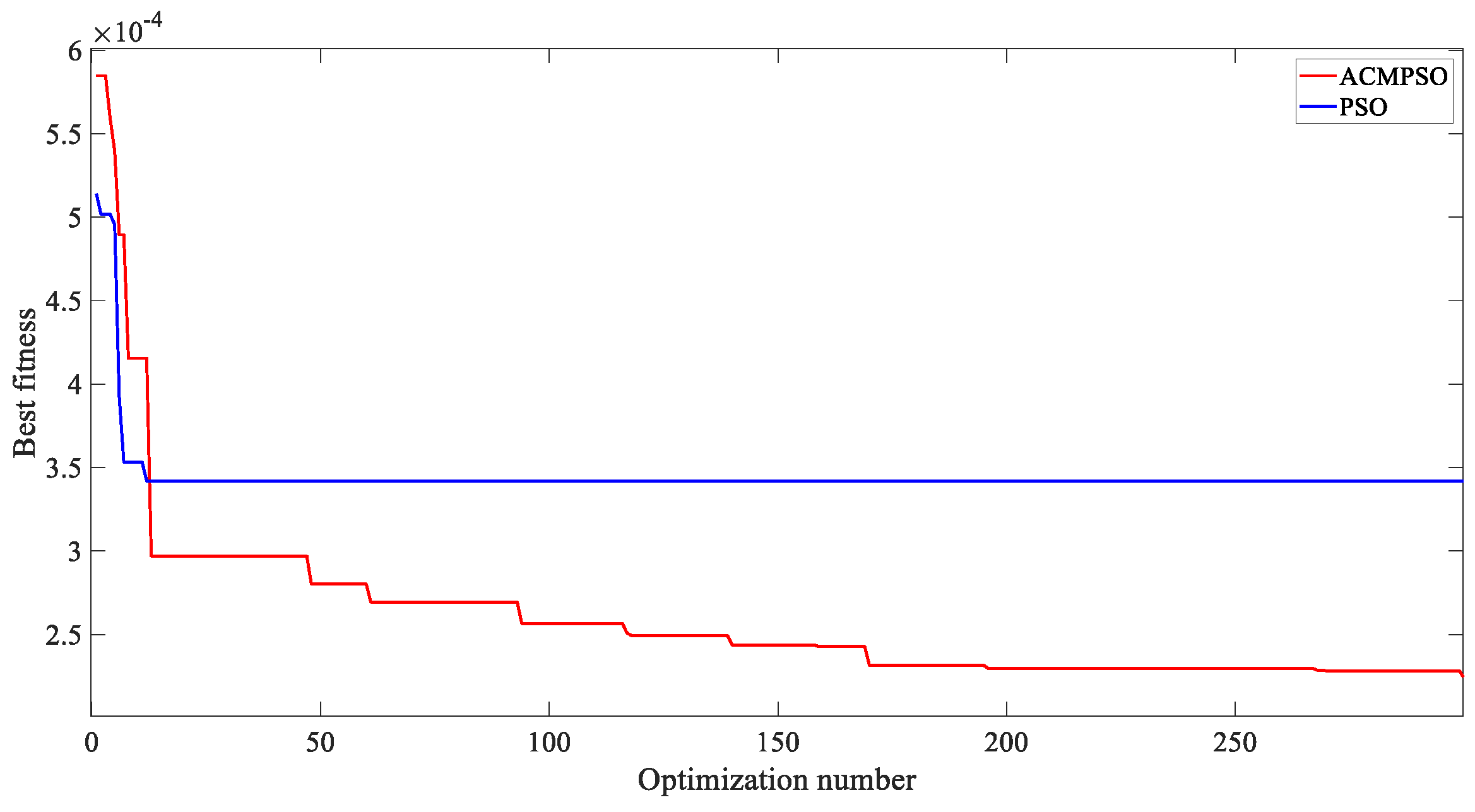
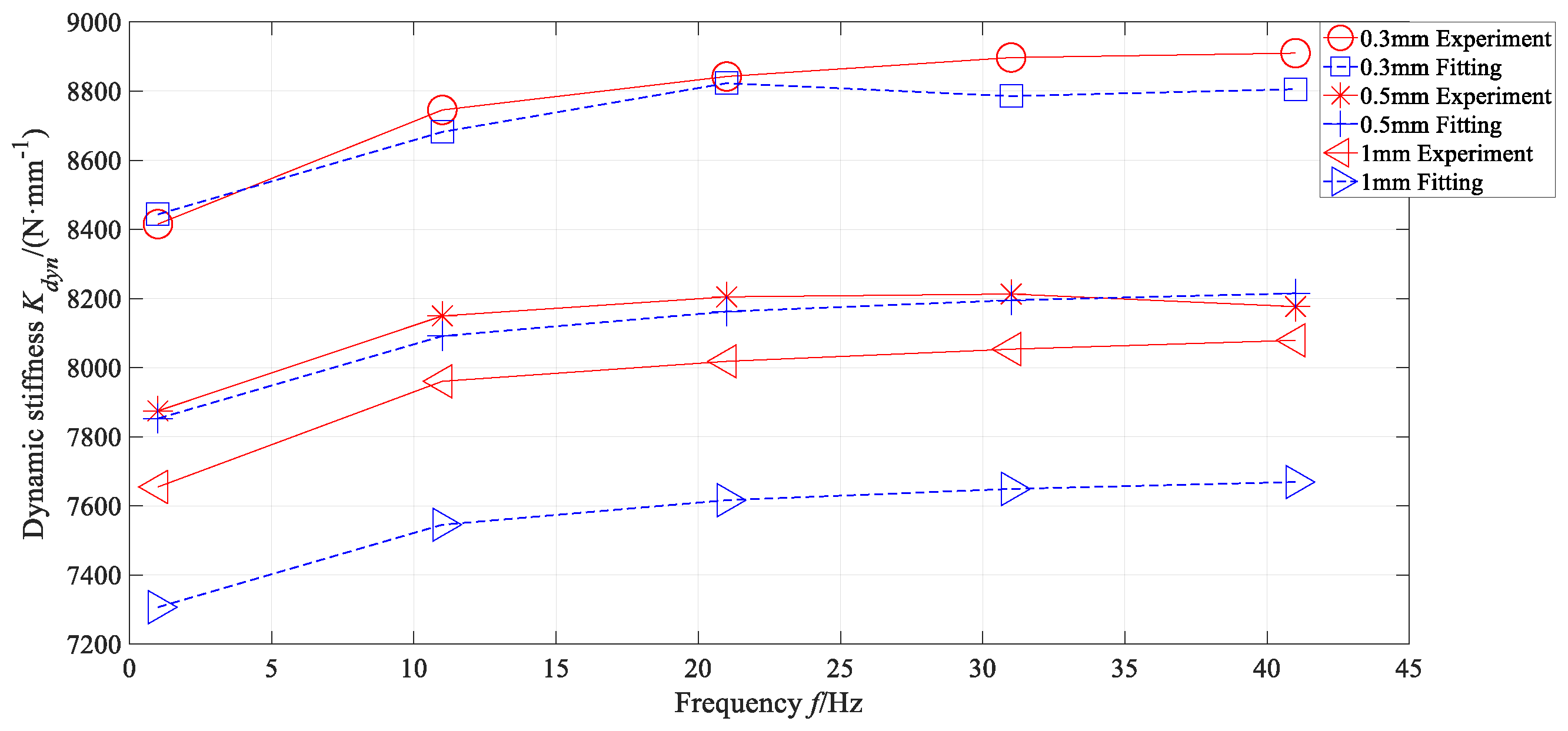
• The proposed combination of the Maxwell and Kelvin–Voigt models for the viscoelastic element in the rear sub-frame rubber bushing dynamic model significantly improves the fitting accuracy to the experimental data after parameter identification using an adaptive chaotic improved particle swarm optimization algorithm.
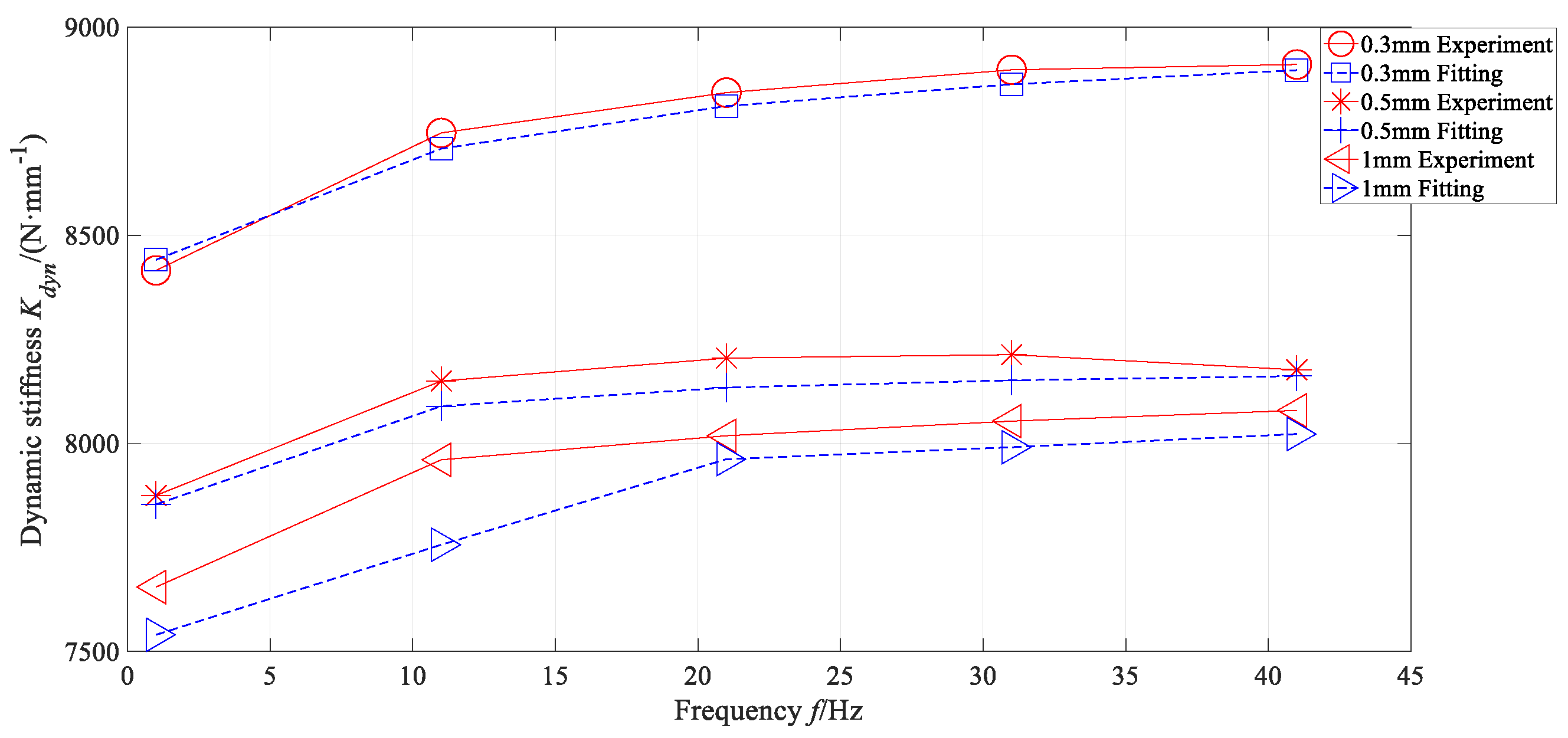
• The sensitivity analysis of the bushing model parameters reveals that recalibrating the $\alpha$, $\beta$, and $k_2$ parameters further enhances the fitting accuracy of the model after re-identification.

References

- Yue, K.; Zhang, Y.; Xu, P. Comparison of Rubber Bushing Models for Loads Analysis; SAE Technical Paper 2021-01-0317; SAE: Warrendale, PA, USA, 2021. [Google Scholar] [CrossRef]
- Ambrósio, J.; Verissimo, P. Improved bushing models for general multibody systems and vehicle dynamics. Multibody Syst. Dyn. 2009, 22, 341–365. [Google Scholar] [CrossRef]
- Guo, R.; Guan, X. A Review of Studies on Rubber Sleeve Dynamic Models; China Society of Automotive Engineers. In Proceedings of 2010 China Society of Automotive Engineers Annual Congress, Shanghai, China, 10–11 June 2010; China Machine Press: Beijing, China, 2010; Volume 4. [Google Scholar]
- Sun, B. Experimental modeling study on dynamic characteristics of rubber spring in engineering vehicle suspension. China Mechanical. Eng. 2006, 17, 1313–1316. [Google Scholar] [CrossRef]
- Dzierzek, S. Experiment-Based Modeling of Cylindrical Rubber Bushings for the Simulation of Wheel; Suspension Dynamic Behavior; SAE Technical Paper 2000-01-0095; SAE: Warrendale, PA, USA, 2000. [Google Scholar] [CrossRef]
- Berg, M. A nonlinear rubber spring model for vehicle dynamics analysis. Veh. Syst. Dyn. 1998, 29, 723–728. [Google Scholar] [CrossRef]
- Zhao, Y.; Hou, Z. Two viscoelastic constitutive models of rubber materials based on fractional derivative. J. Tsinghua Univ. 2013, 53, 378383. [Google Scholar] [CrossRef]
- Metzler, R.; Nonnenmacher, T.F. Fractional relaxation processes and fractional rheological models for the description of a class of viscoelastic materials. Int. J. Plast. 2003, 19, 941–959. [Google Scholar] [CrossRef]
- Bagley, R.L.; Torvik, P.J. On the fractional calculus model of viscoelastic behavior. J. Rheol. 1986, 30, 133–135. [Google Scholar] [CrossRef]
- Lin, S.; Gao, Q.; Li, Y.; Yang, X.; Zhao, X. A viscoelastic constitutive model considering wide temperature, wide frequency and wide dynamic displacement. J. Aerosp. Power 2007, 27, 431–438. [Google Scholar] [CrossRef]
- Liu, J.G.; Xu, M.Y. Higher order fractional constitutive equation of viscoelastic materials involving three different parameters and their relaxation and creep functions. Mech. Time Depend. Mater. 2006, 10, 263–279. [Google Scholar] [CrossRef]
- Gao, Q.; Feng, J.; Zheng, S.; Lin, Y. Study on high-order fractional derivative dynamic model of rubber sleeve. Automot. Eng. 2019, 41, 872–879. [Google Scholar] [CrossRef]
- Zou, K.; Ding, J. Research on parameter identification of robot dynamics. Mach. Tool. Hydraul. 2023, 10–13+18. [Google Scholar] [CrossRef]
- Rivlin, R.S.; Saunders, D.W. Large elastic deformations of isotropic materials. Collect. Pap. R. S Rivin. 1997, 157–194. [Google Scholar]
- Rivlin, R.S. Large elastic deformations of isotropic materials. IV. Further developments of the general theory. Philos. Trans. R. Soc. Lond. Ser. A 1948, 241, 379–397. [Google Scholar]
- Yeoh, O.H. Some forms of the strain energy function for rubber. Rubber Chem. Technol. 1993, 66, 754–771. [Google Scholar] [CrossRef]
- Ogden, R.W. Syntax of referencing. In Non-Linear Elastic Deformations; Ogden, R.W., Ed.; Dover Publication Inc.: Mineola, NY, USA, 1997; p. 221. [Google Scholar]
- Li, G.; Wu, L.; Zhang, S.; Liu, F. Frequency dependence prediction and parameter identification of rubber bushing. Sci. Rep. 2022, 12, 863. [Google Scholar] [CrossRef] [PubMed]
- Manias, S. Non-linear behavior of a rubber isolaror system using fractional derivatives. Veh. Syst. Dyn. 2002, 37, 217–236. [Google Scholar]
- Yang, T. Viscoelastic Theory and Application; Science Press: Beijing, China, 2004. (In Chinese) [Google Scholar]
- Zhang, G.; Zhang, J.; Guo, R.; Gao, Z.; Niu, Y. Dispatch Strategy of Cold-Hot-Electricity Trigeneration System Based on Adaptive Chaotic Particle Swarm Optimization Algorithm. Mod. Electr. Power 2020, 37, 551–558. [Google Scholar] [CrossRef]
- Vuillod, B.; Montemurro, M.; Panettieri, E.; Hallo, L. A comparison between Sobol’s indices and Shapley’s effect for global sensitivity analysis of systems with independent input variables. Reliab. Eng. Syst. Saf. 2023, 234, 109177. [Google Scholar] [CrossRef]