
Simulation of Automobile Structural Member Deformation and Crash via Isogeometric Analysis

 and
and
Abstract
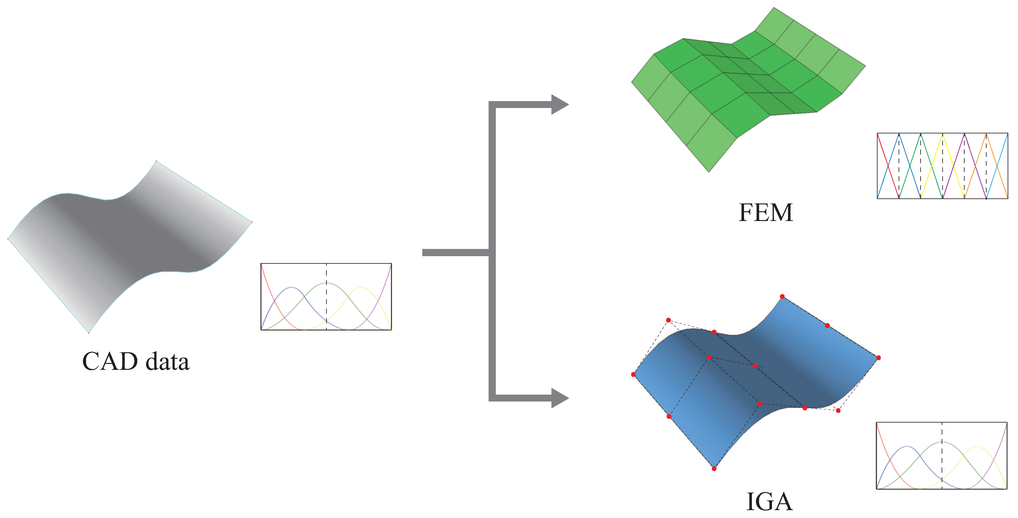
1. Introduction
2. Isogeometric Analysis
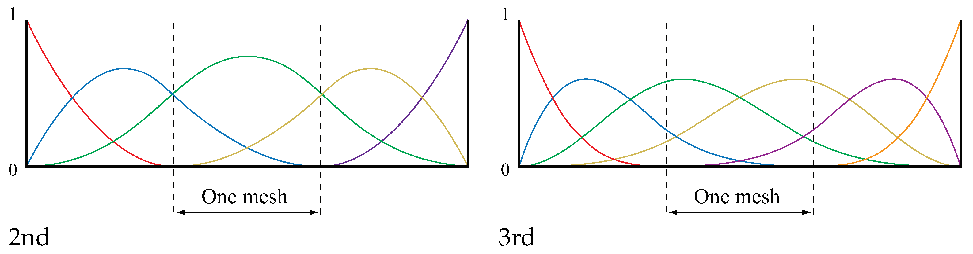
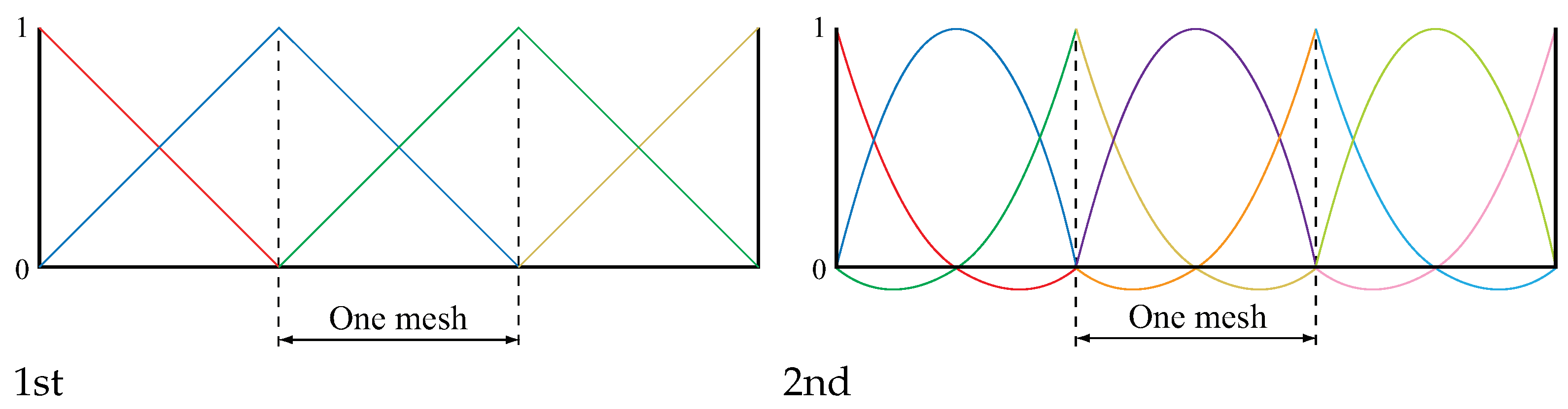
2.1. B-Spline Function
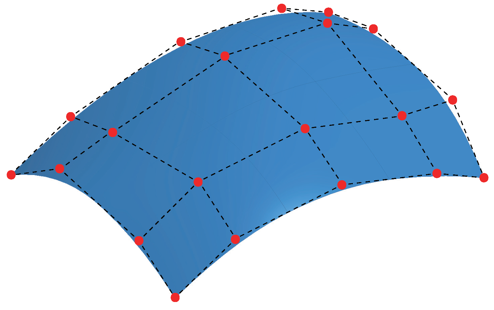
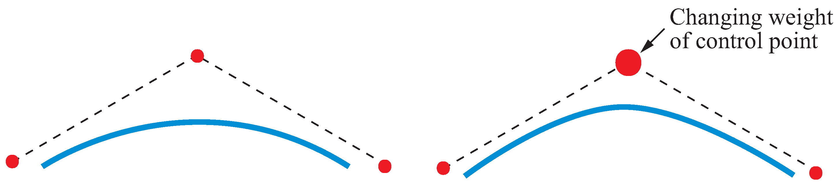
2.2. NURBS Basis Function
2.3. Coordinate Transformation by Mapping
3. Deformation Analysis of Structural Members
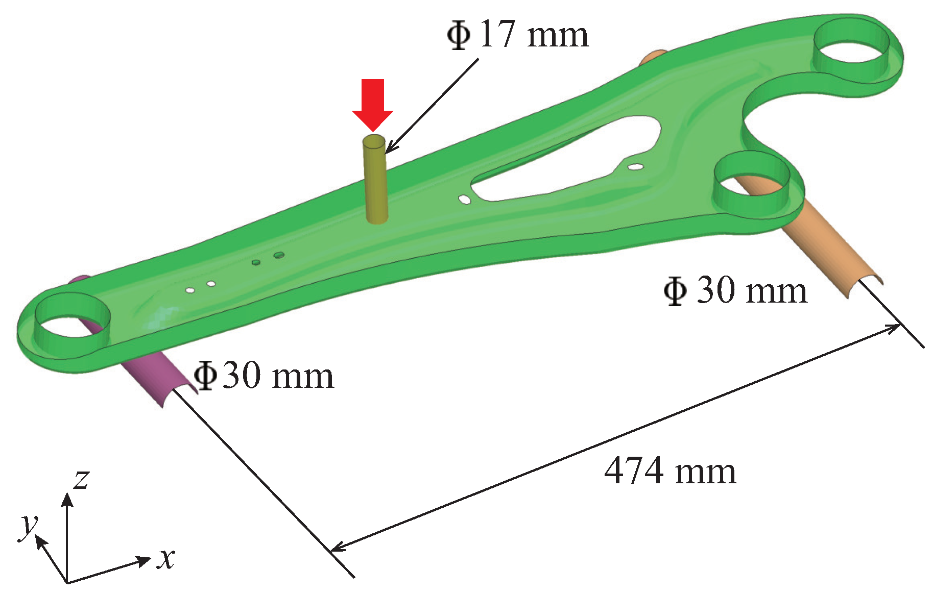
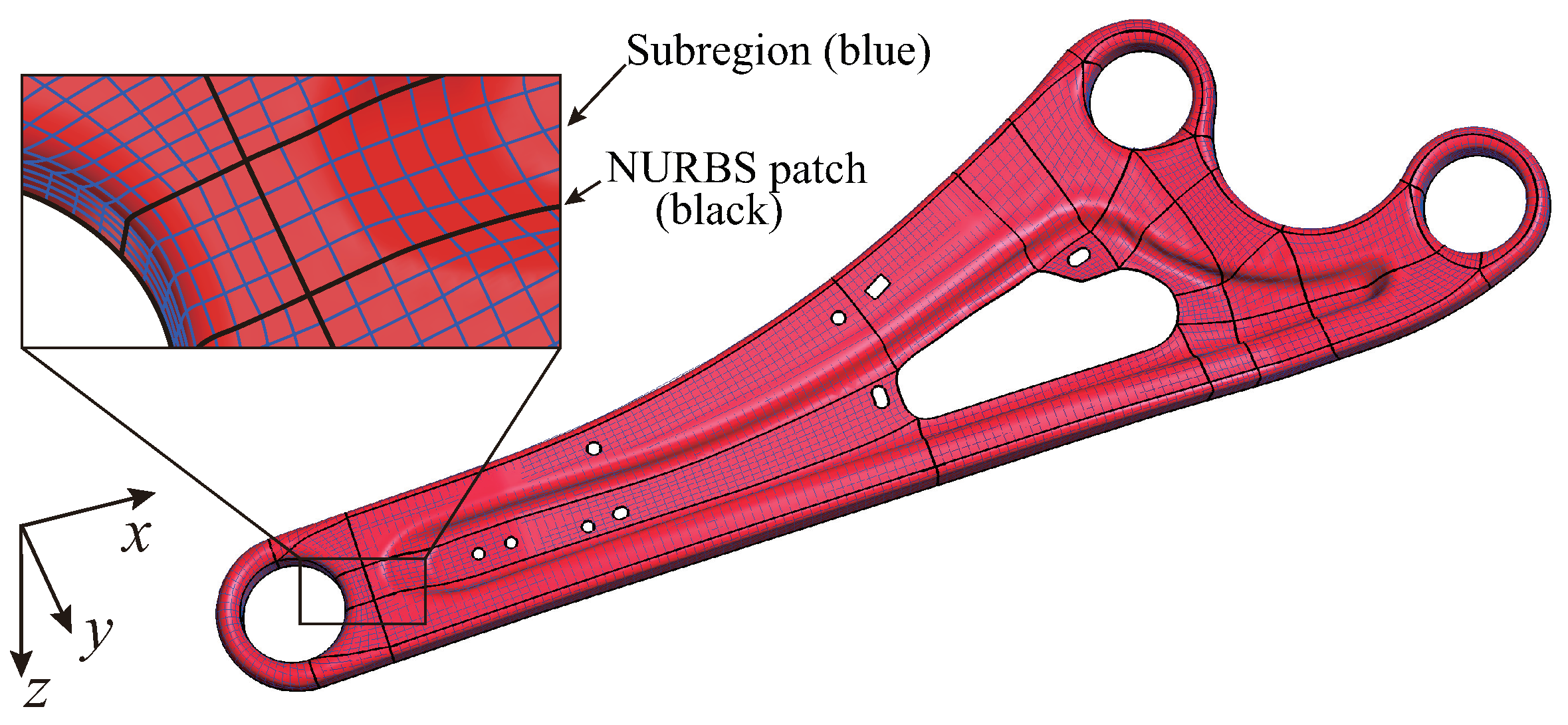
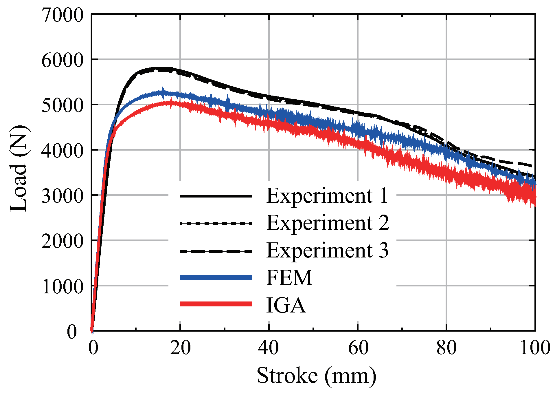
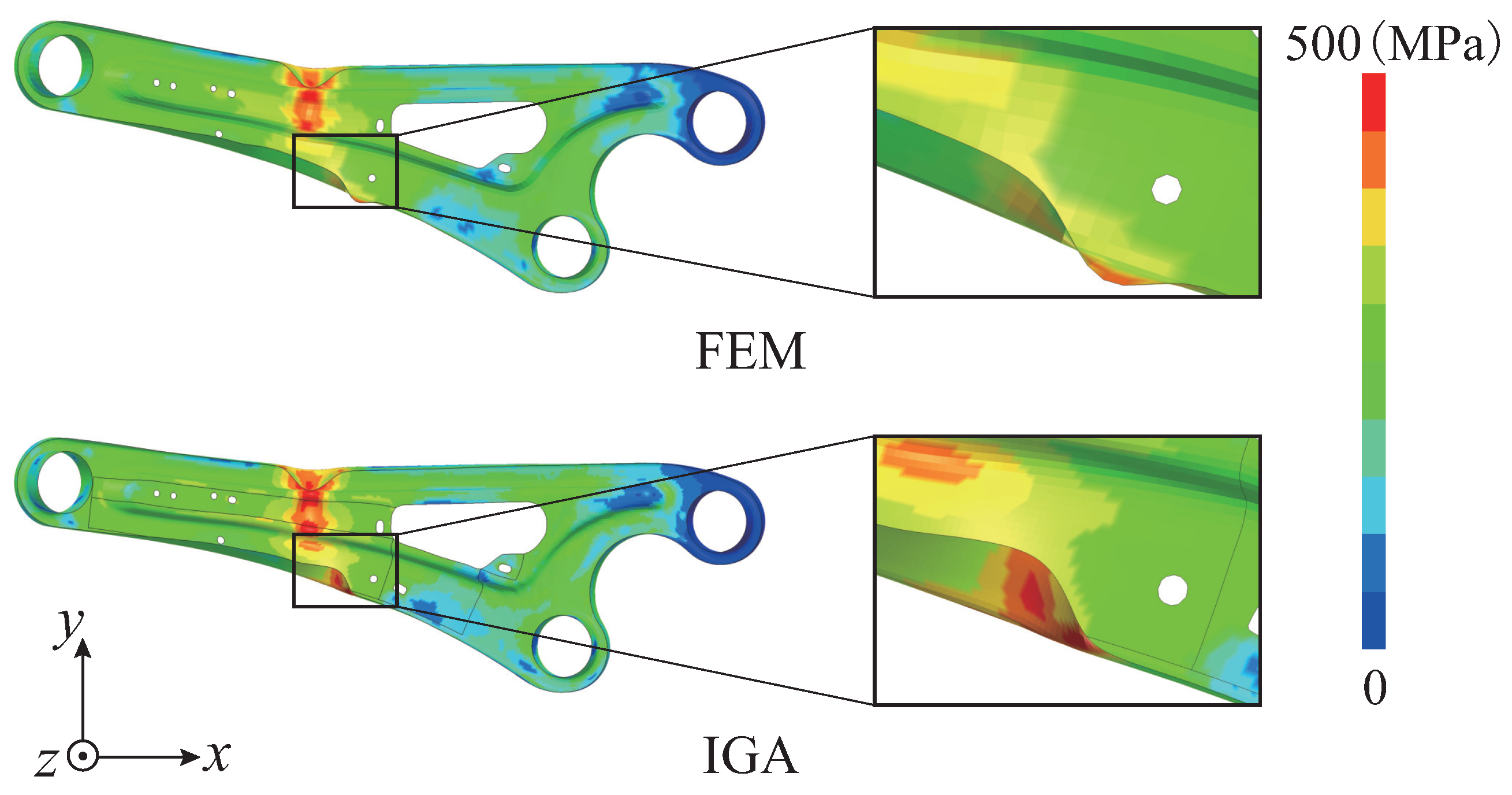
3.1. Three-Point Bending Analysis of Trailing Arm
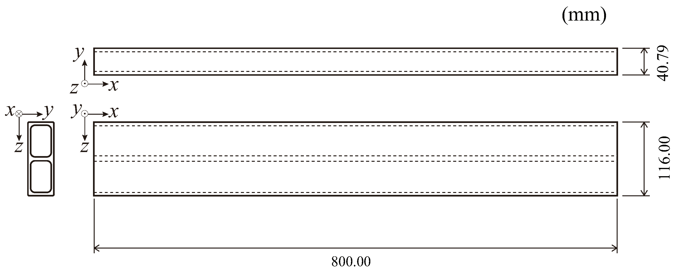
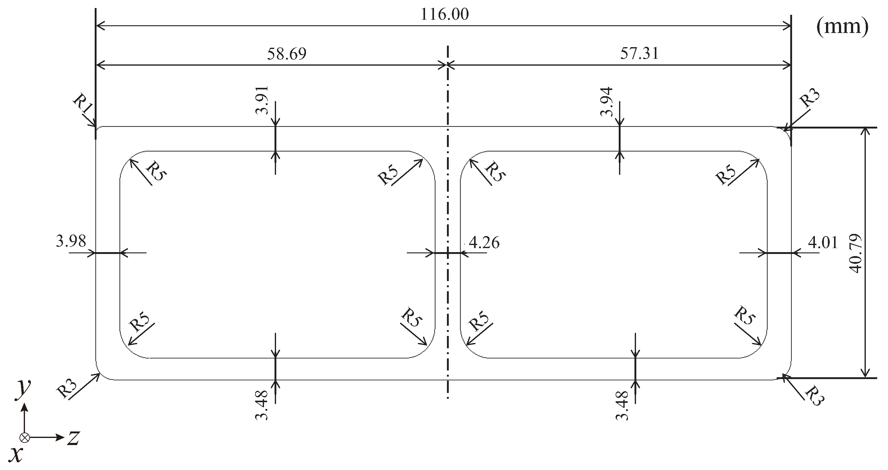
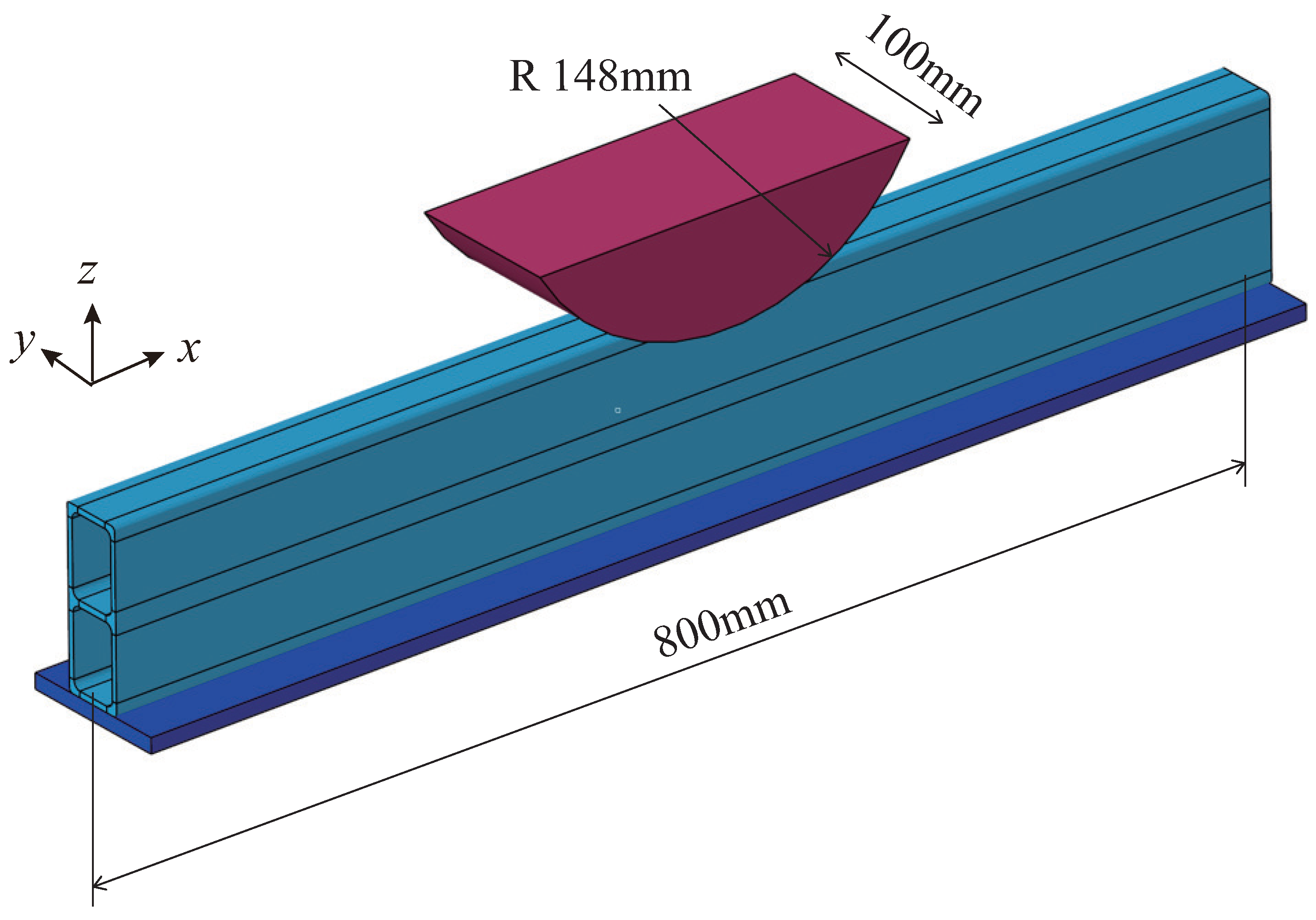
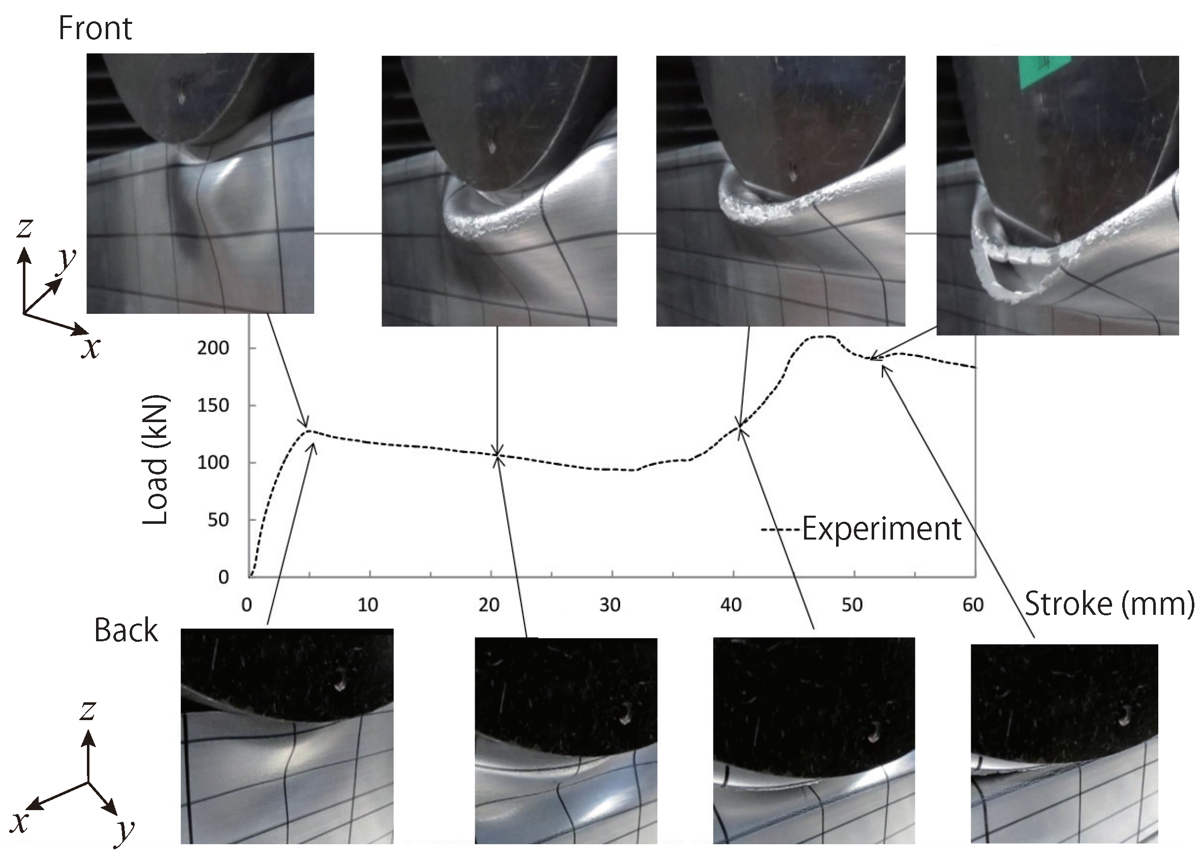
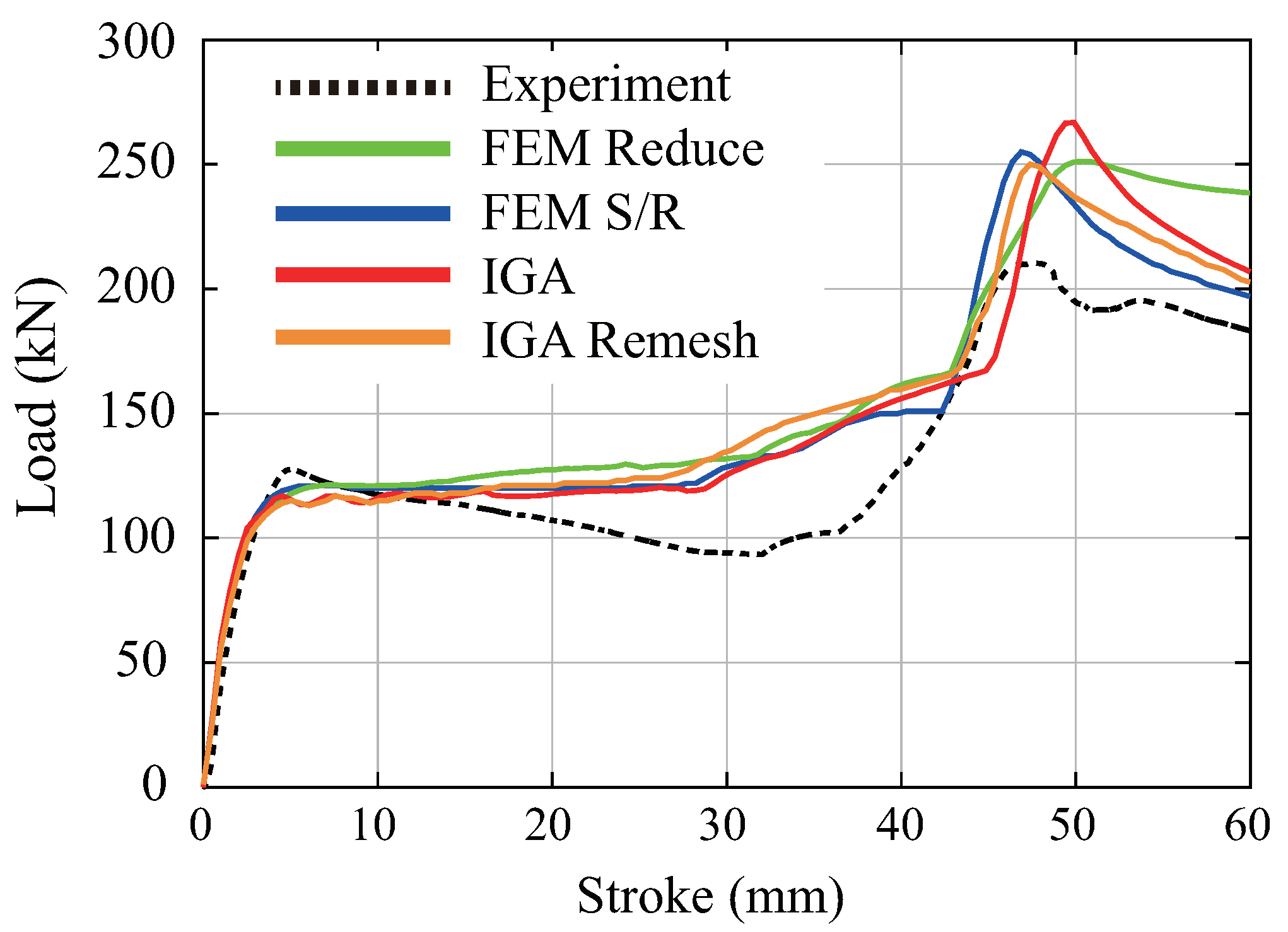
3.2. Compression Analysis of Aluminum Extrusions
4. Crash Analysis of Automobile
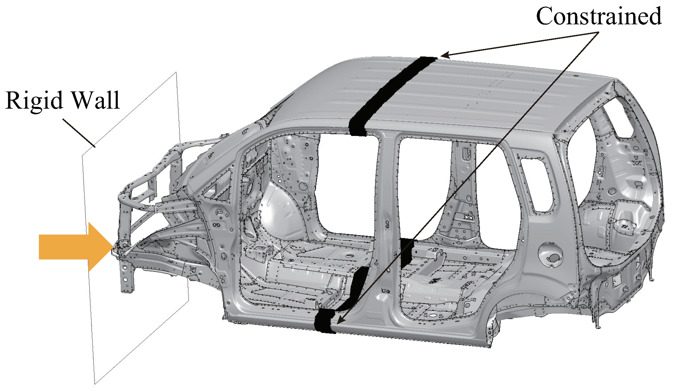
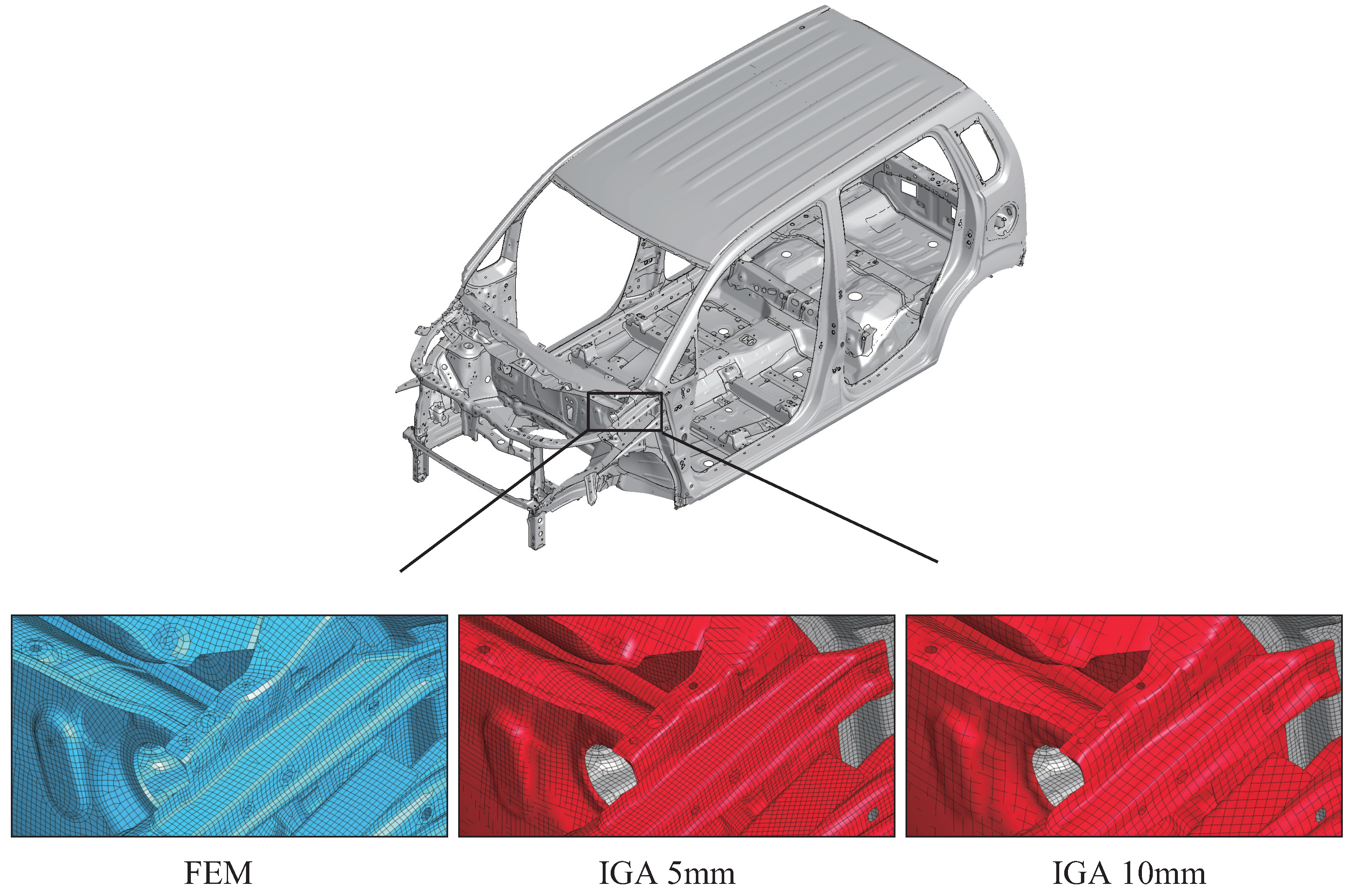
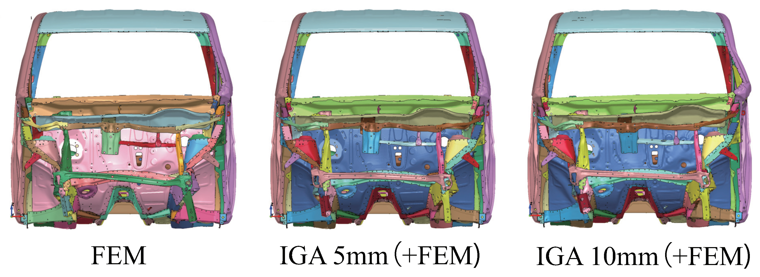
4.1. Automobile Body Model
4.2. Computational Results
4.3. Computational Time
5. Conclusions
Author Contributions
Funding
Conflicts of Interest
References
- Hughes, T.J.R.; Cottrell, J.A.; Bazilevs, Y. Isogeometric analysis, CAD, finite elements, NURBS, exact geometry and mesh refinement. Comput. Methods Appl. Mech. Eng. 2005, 194, 4135–4195. [Google Scholar] [CrossRef]
- Cottrell, J.A.; Hughes, T.J.R.; Bazilevs, Y. Isogeometric Analysis, Toward Integration of CAD and FEA; Wiley: Hoboken, NJ, USA, 2009. [Google Scholar]
- Nagy, A.P.; Benson, D.J. On the numerical integration of trimmed isogeometric elements. Comput. Methods Appl. Mech. Eng. 2015, 284, 165–185. [Google Scholar] [CrossRef]
- Guo, Y.; Ruess, M. Nitsch’s method for a coupling of isogeometric thin shells and blended shell structures. Comput. Methods Appl. Mech. Eng. 2015, 284, 881–905. [Google Scholar] [CrossRef]
- Schuß, S.; Dittmann, M.; Wohlmuth, B.; Klinkel, S.; Hesch, C. Multi-patch isogeometric analysis for Kirchhoff-Love shell elements. Comput. Methods Appl. Mech. Eng. 2019, 349, 91–116. [Google Scholar] [CrossRef]
- Leidinger, L.F.; Breitenberger, M.; Bauer, A.M.; Hartmann, S.; Wuechner, R.; Bletzinger, K.-U.; Duddeck, F.; Song, L. Explicit dynamic isogeometric B-Rep analysis of penalty-coupled trimmed NURBS shells. Comput. Methods Appl. Mech. Eng. 2019, 351, 891–927. [Google Scholar] [CrossRef]
- Leidinger, L.; Hartmann, S.; Benson, D.; Nagy, A.; Rorris, L.; Chalkidis, I. Hybrid IGA/FEM vehicle crash simulations with trimmed NURBS-based shells in LS-DYNA. In Proceedings of the 13th European LS-DYNA Conference, Ulm, Germany, 5–7 October 2021. [Google Scholar]
- Bauer, F.; Yugeng, T.; Leidinger, L.; Hartmann, S. Experience with crash simulations using an IGA body in white. In Proceedings of the 14th European LS-DYNA Conference, Baden-Baden, Germany, 18–19 October 2023. [Google Scholar]
- Morganti, S.; Auricchio, F.; Benson, D.J.; Gambarin, F.I.; Hartmann, S.; Hughes, T.J.R.; Reali, A. Patient-specific isogeometric structural analysis of aortic valve closure. Comput. Methods Appl. Mech. Eng. 2015, 284, 508–520. [Google Scholar] [CrossRef]
- Chen, Y.; Lin, S.P.; Faruque, O.; Alanoly, J.; El-Essawi, M.; Baskaran, R. Current status of LS-DYNA Iso-geometric analysis in crash simulation. In Proceedings of the 14th International LS-DYNA Users Conference, Dearborn, MI, USA, 12–14 June 2016. [Google Scholar]
- Hartmann, S.; Nagy, A.P.; Benson, D.J. Advances in IGA for sheet metal forming applications. In Proceedings of the 11th European LS-DYNA Users Conference, Salzburg, Austria, 9–11 May 2017. [Google Scholar]
- Hartmann, S.; Benson, D.J. Mass scaling and stable time step estimates for isogeometric analysis. Int. J. Numer. Methods Eng. 2015, 102, 671–687. [Google Scholar] [CrossRef]
- Casquero, H.; Bona-Casas, C.; Gomez, H. A NURBS-based immersed methodology for fluid-structure interaction. Comput. Methods Appl. Mech. Eng. 2015, 84, 943–970. [Google Scholar] [CrossRef]
- Caseiro, J.F.; Valente, R.A.F.; Reali, A.; Kiendl, J.; Auricchio, F.; Alves de Sousa, R.J. Assumed natural strain NURBS-based solid-shell element for the analysis of large deformation elasto-plastic thin-shell structures. Comput. Methods Appl. Mech. Eng. 2015, 284, 861–880. [Google Scholar] [CrossRef]
- Kiendl, J.; Hsu, M.C.; Wu, M.C.; Reali, A. Isogeometric Kirchhoff-Love shell formurations for general hyperelastic materials. Comput. Methods Appl. Mech. Eng. 2015, 291, 280–303. [Google Scholar] [CrossRef]
- Hu, P.; Hu, Q.; Xia, Y. Order reduction for locking free isogeometric analysis of Timoshenko beams. Comput. Methods Appl. Mech. Eng. 2016, 308, 1–22. [Google Scholar] [CrossRef]
- Piegl, L.; Tiller, W. The NURBS Book; Springer: Berlin/Heidelberg, Germany, 1997. [Google Scholar]
- LS-DYNA theory Manual, Livermore Software Technology (LST), An ANSYS Company. 2023. Available online: https://lsdyna.ansys.com/manuals/ (accessed on 8 April 2024).
- Pian, T.H.H.; Sumihara, K. Rational approach for assumed stress finite elements. Int. J. Numer. Methods Eng. 1984, 20, 1685–1695. [Google Scholar] [CrossRef]
- Simo, J.C.; Hughes, T.J.R. On the variational foundations of assumed strain methods. J. Appl. Mech. 1986, 53, 51–54. [Google Scholar] [CrossRef]


| FEM Reduce | FEM S/R | IGA | IGA Remesh | |
|---|---|---|---|---|
| Time increment | 1.18 × 10⁻⁷ | 1.18 × 10⁻⁷ | 8.51 × 10⁻⁸ | 2.21 × 10⁻⁷ |
| Computational time | 6504 | 13,903 | 30,830 | 14,033 |
| FEM | IGA 5 mm (+FEM) | IGA 10 mm (+FEM) |
|---|---|---|
| 9227 | 19,455 | 10,952 |
Disclaimer/Publisher’s Note: The statements, opinions and data contained in all publications are solely those of the individual author(s) and contributor(s) and not of MDPI and/or the editor(s). MDPI and/or the editor(s) disclaim responsibility for any injury to people or property resulting from any ideas, methods, instructions or products referred to in the content. |
© 2024 by the authors. Licensee MDPI, Basel, Switzerland. This article is an open access article distributed under the terms and conditions of the Creative Commons Attribution (CC BY) license (https://creativecommons.org/licenses/by/4.0/).
Share and Cite
Yokoyama, Y.; Nagasaka, K.; Masuda, I.; Sugiyama, H.; Okazawa, S. Simulation of Automobile Structural Member Deformation and Crash via Isogeometric Analysis. Vehicles 2024, 6, 967-983. https://doi.org/10.3390/vehicles6020046
Yokoyama Y, Nagasaka K, Masuda I, Sugiyama H, Okazawa S. Simulation of Automobile Structural Member Deformation and Crash via Isogeometric Analysis. Vehicles. 2024; 6(2):967-983. https://doi.org/10.3390/vehicles6020046
Chicago/Turabian StyleYokoyama, Yuta, Kei Nagasaka, Idemitsu Masuda, Hirofumi Sugiyama, and Shigenobu Okazawa. 2024. "Simulation of Automobile Structural Member Deformation and Crash via Isogeometric Analysis" Vehicles 6, no. 2: 967-983. https://doi.org/10.3390/vehicles6020046
APA StyleYokoyama, Y., Nagasaka, K., Masuda, I., Sugiyama, H., & Okazawa, S. (2024). Simulation of Automobile Structural Member Deformation and Crash via Isogeometric Analysis. Vehicles, 6(2), 967-983. https://doi.org/10.3390/vehicles6020046