Conceptual Study on Car Acceleration Strategies to Minimize Travel Time, Fuel Consumption, and CO₂-CO Emissions

Abstract

A conceptual study was performed on intelligent driving acceleration strategies for vehicles equipped with internal combustion engines. Two archetypal acceleration scenarios of highway driving and urban driving were prescribed. Three trajectories were considered for each scenario. They involved (a) nearly constant acceleration, (b) fast acceleration first and slow acceleration later, and (c) slow acceleration first and fast acceleration later. The selected vehicle was a generic European small–medium passenger car. Engine inlet pressure and ignition time were optimized along each trajectory to minimize fuel consumption, CO, and CO₂ emissions, and travel time. The optimization process involved a methodological approach based on the higher-order singular value decomposition of the tensor form of the engine model. The optimized trajectories were analyzed and compared among themselves. Conceptual acceleration design guidelines for intelligent driving were provided that could be of interest when integrating vehicle/engine performance into the surrounding traffic flow.

1. Introduction

1.1. Overview

Reducing fuel consumption and pollutant emissions are critical issues for internal combustion engines in the context of car intelligent driving (including the case of battery electric–hybrid vehicles). The reason is that transition to fully electric or hydrogen-based transport systems may take longer than expected. During this transition, highly efficient optimized vehicles based on internal combustion engines may represent a feasible compromise.

The operation procedure of an internal combustion engine begins with a certain power demand that depends on the vehicle trajectory, and follows with an adjustment of the engine control parameters to satisfy that demand. This means that fuel consumption and pollutant emissions depend on both external (vehicle trajectory) and internal (engine variables) factors that, in turn, depend on a large number of parameters.

In this context of complex operation, it is doubtful that a human driver would be able to develop real time strategies to deal, optimally, with a non-linear problem that contains a large set of variables. Nowadays, the prevailing trend in the field is to move towards intelligent driving strategies by means of either using driver assisting engine control unit (ECU) software, or by trying to move to an autonomous concept vehicle. Intelligent driving approaches are very promising but require a large amount of R&D effort. The reason is that they involve (a) modelization of vehicle powerplant and associated mechanical and electrical/electronic systems, (b) development of a driving framework for a variety of drivers and trajectories, and interaction with other drivers, and (c) integration of said models into an optimization structure preferably able to work in real time. Recent examples of studies in the area could be found in the works of Langhorst et al. [1], Li et al. [2], and Diachuk and Easa [3,4].

One variable that appears ubiquitously in the R&D activities dealing with intelligent driving is vehicle acceleration. The reasons are twofold: (a) acceleration has a direct impact on traffic flow behavior; and (b) acceleration plays a critical role in the vehicle dynamic equation and, therefore, on the demanded engine power, thereby affecting fuel consumption and emissions.

1.2. Literature Review

Regarding the relation between acceleration and traffic flow, Choudhury and Islam, [5] have developed a “Latent Leader” approach to model the influence that acceleration decisions have in traffic streams with weak lane discipline (meaning that the driver may have several vehicles in front, and not necessarily a leader vehicle). In their conclusions, the authors point to the importance of space headway in a situation of vehicle deceleration. Goñi-Ros et al. [6] addressed traffic flow optimization at sags by means of acceleration control. Their results show that the optimal solution involves a deceleration–acceleration–deceleration–acceleration strategy. Ivanchev et al. [7] have studied available models of autonomous vehicle longitudinal acceleration in a context of mixed traffic (autonomous vehicles mixed with human drivers) to maximize the speed, safety, comfort, and efficiency of the vehicle population. For this aim, they formulated a multi-objective problem, and found the set of traffic/driving parameters that optimized a certain objective function. Interestingly enough, they state that the most important limitation of their study is the reliability of the human model. Manolis et al. [8] have presented an adaptive-cruise-control-based strategy for traffic flow efficiency. This is achieved in real time, acting on the driving behavior (including acceleration strength). In their conclusions, increased acceleration at active bottlenecks was presented as one of the optimal strategies. Wang et al. [9] have studied how road curvature ahead and slope variations affect driver’s deceleration and acceleration decisions.

Concerning the effect of acceleration on engine performance parameters, Ard et al. [10] present a car-following algorithm that controls acceleration strategies and reduces the engine fuel and/or electric consumption. In their conclusions, the authors report a 30% energy improvement as compared to a realistically calibrated human driver. It is important to note that, in addition to simulations, the authors used specifically adapted experimental vehicles: a gasoline Mazda CX-7, and an electric Nissan Leaf. Bishop et al. [11] developed engine maps of fuel consumption and emissions associated with some specific transient driving cycles. To this aim, they used data provided by the on-board diagnostic system in combination with a dynamic equation of the vehicle that included acceleration and a portable emissions measurement system. Some of their experimental vehicles were a Volkswagen Golf and a Chevrolet Cruze. Guo et al. [12] have developed a hybrid reinforcement learning eco-driving algorithm that accounts for longitudinal acceleration and deceleration as well as for lateral lane-changing maneuvers. The objectives of the algorithm were twofold: (a) to reduce fuel consumption, and (b) to maintain an acceptable travel time. Hibberd et al. [13] tested two haptic accelerator pedal systems, and one multimodal visual–auditory system to develop guidelines related to the fuel efficiency of the accelerator pedal position in the context of an eco-driving in-vehicle assistance system. The study used the driving simulator at Leeds University and considered several scenarios: deceleration (96 km/h to 64 km/h), cruise (64 km/h), and acceleration (64 km/h to 96 km/h). Sun et al. [14] developed a method to estimate vehicle emissions and energy consumption using mobile sensing data and specific vehicle trajectories (microflow). The considered trajectories accounted not only for the traffic state such as queuing and free-flowing, but also for the vehicle driving mode: cruise, idle, acceleration, and deceleration. Tsanakas et al. [15] proposed a method to estimate emissions and fuel consumption using the so-called virtual vehicle trajectories, which are generated out of partially observed traffic data. The engine/car data used in the study followed the previous work of Hausberger et al. [16]. These authors experimentally categorized seven different gasoline cars and generated engine maps that included emissions information. The steady experimental maps were corrected, whenever applicable, with so-called transient emission correction factors relevant for transient driving cycles. In their conclusions, Tsanakas et al. [15] provided guidelines to improve the virtual vehicle trajectories technique, and stated a possible range of applications not necessarily related to emission-modelling. Recent experimental studies, performed at both test benches and actual traffic conditions, that relate emission characteristics to acceleration have been published by Kim et al. [17], Chadrashekar et al. [18], and Kuppili et al. [19]. In this context, a very comprehensive semi-empirical methodology to link instantaneous acceleration and CO₂ emissions has been published by Suarez et al. [20]. Also, it is relevant to refer to the work of Zhang et al. [21], which studied the influence of acceleration on vehicle emissions at intersections using the MOVES emission model (US Environmental Protection Agency, 2009) [22].

Finally, it is relevant to refer to the study presented by Blokpoel et al. [23]. The authors focused on the problem of vehicle emissions when stopping and accelerating at traffic lights. The authors began the article by stating that this specific driving condition is one of the main contributing factors to vehicle emissions in urban environments. Then, they presented an adaptive control strategy to minimize CO₂ emissions at traffic lights. The outcome could be summarized as a series of interesting guidelines. First, emissions optimum ratio of delay time versus stops should be 1:165 at 50 km/h. Second, at 70 km/h speed limit, the ratio increases to 1:296. Since it was found that optimal free flow speed was 70 km/h, the maximum speed for optimal emissions with long distances between intersections and not many stops should be higher than 50 km/h.

1.3. The Present Study

In line with the references discussed above, the novelty of the present study is that it provides some conceptual guidelines for a somewhat idealized problem. The problem is when accelerating along a longitudinal trajectory, what is the best strategy to minimize fuel consumption and emissions while maintaining a reasonable travel time? To accelerate fast first and slow later? The opposite? Or something intermediate? An additional methodological novelty is the use of higher-order singular value decomposition (HOSVD) for generalization and densification of engine output data that, otherwise, may require an enormous computational effort. It should be remarked, nonetheless, that this study is of a conceptual nature. The aim is to first carry out an exploratory analysis based on a new methodology. As a second step in the near future, a series of additional practical aspects such as wear of certain components, quality of fuel, engine temperature, vehicle maintenance, shift behavior, gearbox, etc., will be considered. One example of the importance of these effects could be found in Crolla [24], where the influence of rolling resistance was highlighted in urban driving.

Regarding organization of the manuscript, the problem is described first (Section 2). Next, the methodology to solve the problem based on the minimization of a multi-objective function (Section 3) is described. Results are presented and discussed in Section 4, and, finally, conclusions and guidelines are given in Section 5.

2. Problem Description

2.1. Problem Definition

The problem consisted of the evaluation of different vehicle trajectories in two acceleration scenarios representative of highway and urban driving. The comparison was performed in terms of fuel consumption, CO₂ and CO emissions, and time needed to cover the trajectories.

Each acceleration scenario had its own constant transmission ratio. The first acceleration scenario (AC1) was high transmission ratio (highway driving), while the second (AC2) was low transmission ratio (urban driving). Three different trajectories (T1, T2, T3) were defined for each scenario. They involved nearly constant acceleration (T1), fast acceleration first and slow acceleration later (T2), and slow acceleration first and fast acceleration later (T3).

For each scenario and trajectory, two engine input parameters, inlet pressure and ignition timing, were optimized as a function of time along the trajectory to minimize four output parameters. The reason for this selection is that inlet pressure and ignition timing are two typical parameters that are acted upon by the engine control unit in a context of intelligent driving (they have a large influence on the thermodynamics cycle). The methodology is, however, generic and could accommodate other sets or input parameters. The output parameters were total fuel consumption, total emissions of both CO and CO₂, and driving time along the trajectory. A restriction of the optimization process was to keep an acceptable risk of engine knocking. Then, the optimized trajectories were compared among themselves to extract generic guidelines regarding vehicle acceleration strategies.

2.2. The Car

A representative small–medium segment European type gasoline car was selected. Its relevant architectural and operational parameters were:

• Mass (m): 1150 kg;
• Front surface area (Af): 2 m²;
• Drag coefficient (CD): 0.33;
• Maximum power (W): 90 kW;
• Maximum crankshaft rotating speed: 5500 rpm;
• Cylinders: four in line;
• Piston diameter (b); 77 mm;
• Crank length (LC): 43 mm;
• Connecting rod length (LCR): 144 mm;
• Total displacement: 1600 cm³;
• Compression ratio: 11:1;
• Total moment of inertia of rotating parts (I_R): 0.55 kg·m²;
• Admission valve closing: 50 deg after bottom dead center;
• Exhaust valve opening: 50 deg before top dead center

2.3. Acceleration Scenarios

Two acceleration scenarios were considered. The first (AC1) addressed acceleration at velocities of the order of 100 km/h along a horizontal plane with a high transmission ratio. The second (AC2) considered acceleration at velocities of the order of 30 km/h along an inclined plane with 5% slope with a low transmission ratio. There is, certainly, some level of arbitrariness in this selection since there is an enormous variety in possible acceleration trajectories in the context of either urban or highway traffic scenarios. However, what is intended is to select some trajectories that may illustrate the development of the methodology while being reasonably representative of the traffic scenarios.

Three different trajectories were defined for each acceleration scenario.

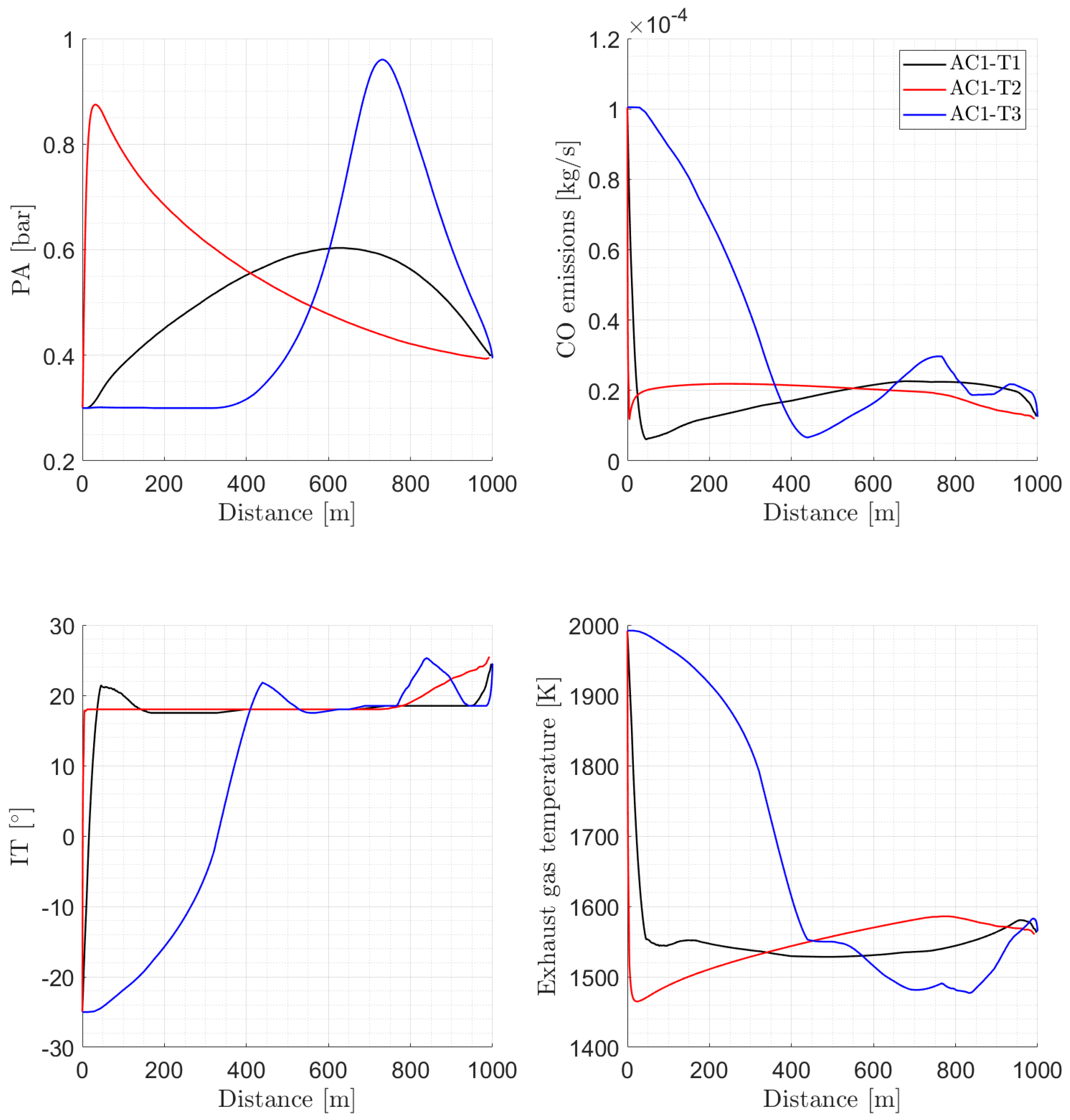
2.3.1. Acceleration Scenario 1

• The car accelerated from 20 m/s (72 km/h) up to 35 m/s (126 km/h) along a horizontal plane 1000 m long, see Figure 1;
• Acceleration at both the beginning and end points was zero;
• Three velocity trajectories (time laws) were considered. They were modelled via Bezier polynomials, and represented nearly constant acceleration (T1), fast acceleration first and slow acceleration later (T2), and slow acceleration first and fast acceleration later (T3). Each Bezier polynomial had 1000 points;
• The transmission ratio was 23 km/h per 1000 rpm.

The idealized dynamic equation of the vehicle in this case (neglecting friction and rolling resistance) was:

$${\dot{W}}_{engine}=\frac{1}{2}\rho A_f{C}_D{v}^3+\frac{d}{dt}\left(\frac{1}{2}m{v}^2\right)+\frac{d}{dt}\left(\frac{1}{2}{I}_R{\omega }^2\right)$$

(1)

The term on the left, ${\dot{W}}_{engine}$, is the engine power. The first term on the right is the power needed to overcome the aerodynamic drag ($\rho$ is the air density, $v$ the vehicle velocity). The third and fourth terms represent the power required to accelerate the vehicle and the engine rotating parts, respectively ($\omega$ is the rotational velocity of the rotating parts, and $I_R$ the generalized moment of inertia). For each trajectory, $v$ is known as a function of time (and $\omega$ is known, too, via the transmission ratio). Then, the acceleration is known, and the required engine power, ${\dot{W}}_{engine}$, is obtained from Equation (1). Figure 1 shows the relevant parameters: velocity, acceleration, required engine power, and covered distance as a function of time, for the three trajectories T1, T2, and T3 of scenario AC1.

The value of the parameters at both starting and end points of the trajectories are given in

Table 1. Vehicle velocity, RPM, engine power, distance covered, fuel consumption, and pollutants emissions at the starting and end points of trajectories in acceleration scenario AC1.

	Starting Point	End Point
Velocity [m/s]	20	35
RPM	3129	5483
Power [kW]	3.2	16.3
Distance [m]	0	1000
C [kg/s]	0.89 × 10−3	2.01 × 10−3
CO2 [kg/s]	2.57 × 10−3	6.15 × 10−3
CO [kg/s]	0.100 × 10−3	0.012 × 10−3

(they are the same for all trajectories within the acceleration scenario AC1).

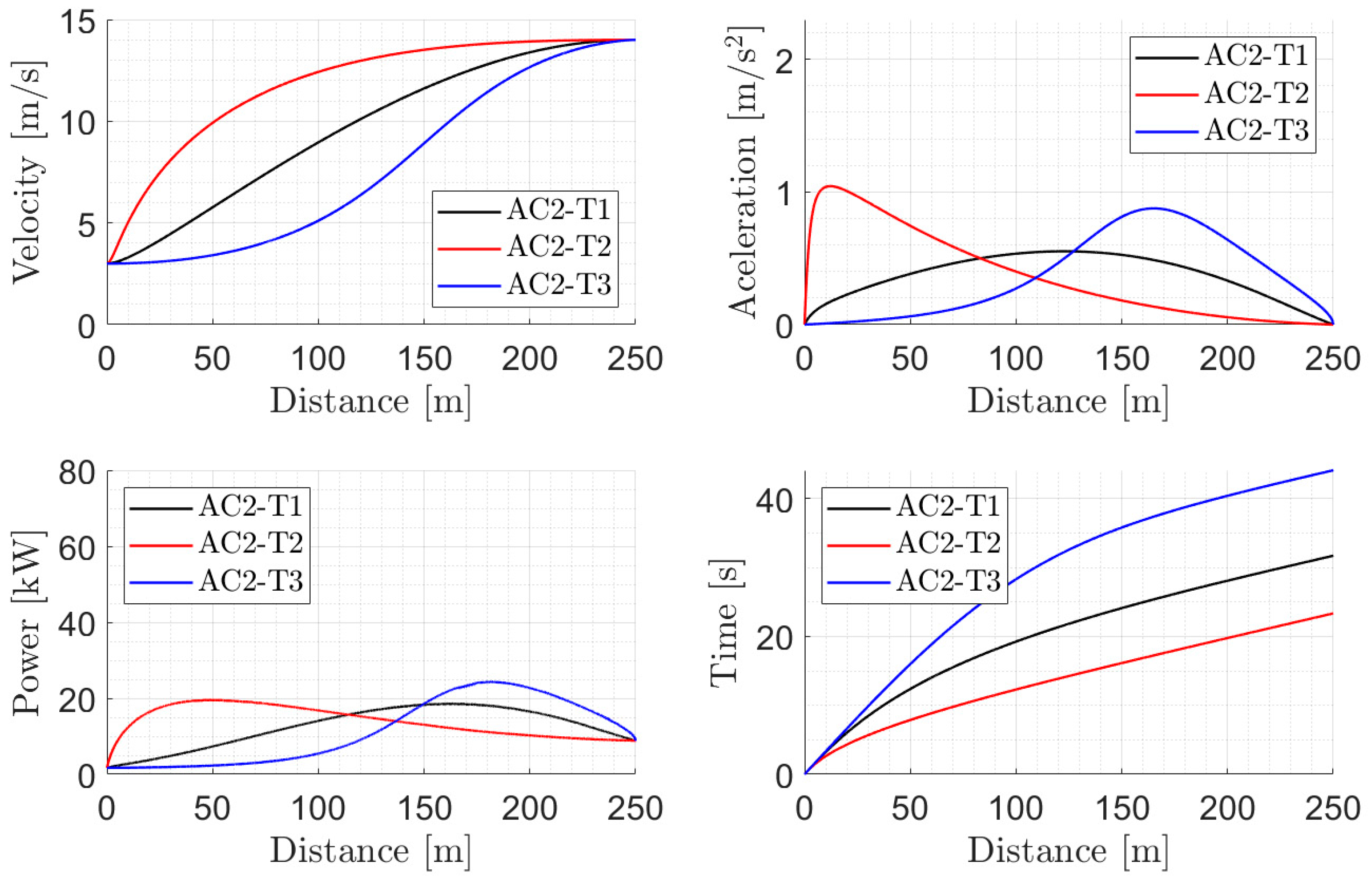
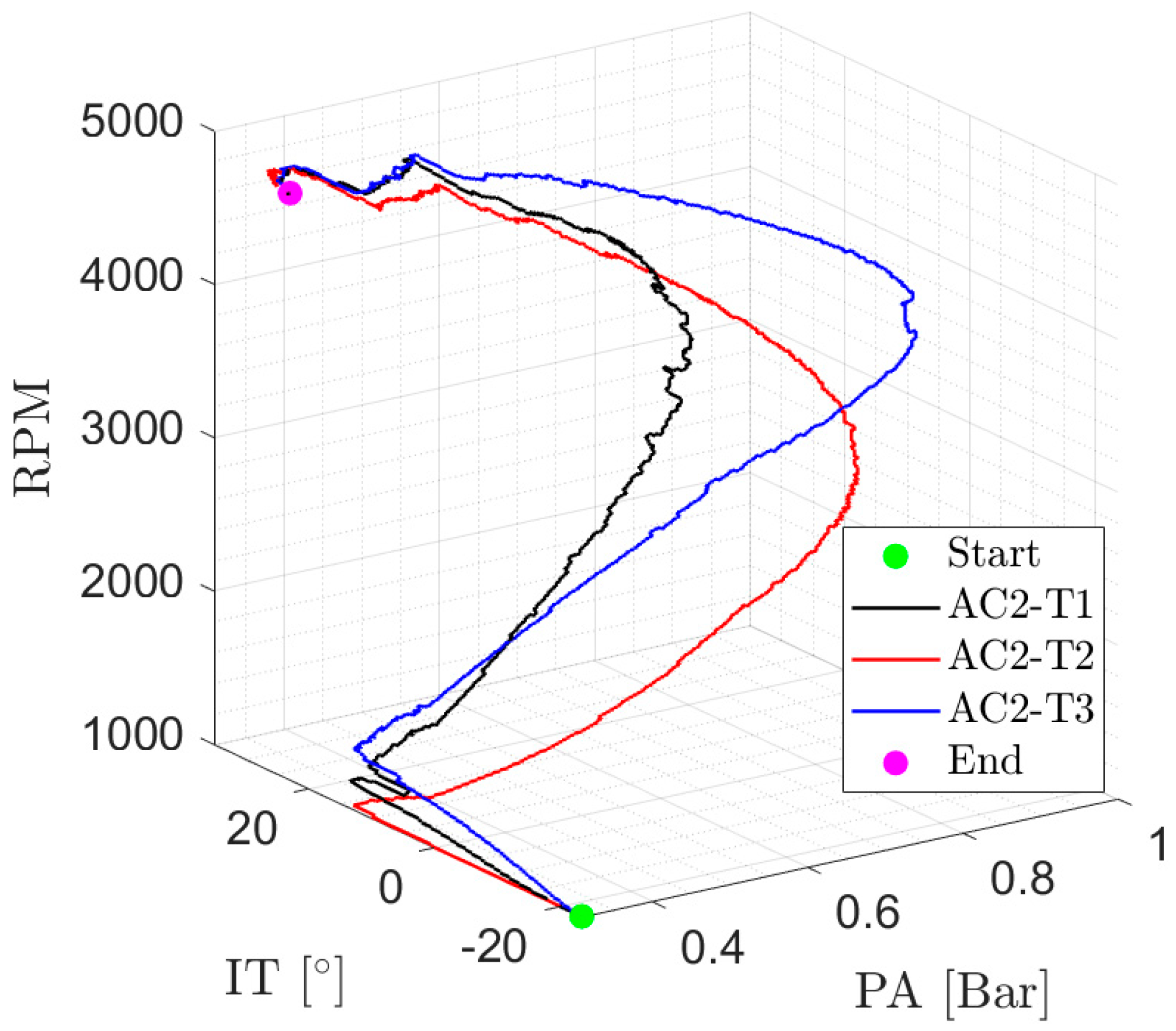
2.3.2. Acceleration Scenario 2 (AC2)

The outlook of scenario 2 is similar to that of scenario 1, but for three differences:

• The car accelerated from 3 m/s (11 km/h) to 14 m/s (50 km/h) along an inclined plane (5% slope) 250 m long, see Figure 2;
• The transmission ratio was 10.8 km/h per 1000 rpm;
• An additional term was included in the right-hand side of Equation (1) to account for the gain of potential energy per unit time when climbing the slope:

$${\dot{W}}_{engine}=\frac{1}{2}\rho A_f{C}_D{v}^3+\frac{d}{dt}\left(\frac{1}{2}m{v}^2\right)+\frac{d}{dt}\left(\frac{1}{2}{I}_R{\omega }^2\right)+\frac{d}{dt}\left(gmz\right)$$

(2)

where g, m, and z are gravity acceleration, vehicle mass, and height. Figure 2 presents the relevant trajectory parameters of acceleration scenario 2 (AC2).

Parameters at the beginning and end of the trajectories are presented in

Table 2. Vehicle velocity, RPM, engine power, distance covered, fuel consumption, and pollutants emissions at the starting and end point of trajectories in acceleration scenario AC2.

	Starting Point	End Point
Velocity [m/s]	3	14
RPM	1000	4669
Power [kW]	1.7	8.8
Distance [m]	0	250
C [kg/s]	0.30 × 10−3	1.59 × 10−3
CO2 [kg/s]	0.86 × 10−3	4.88 × 10−3
CO [kg/s]	0.026 × 10−3	0.004 × 10−3

.

3. Methodology

3.1. Overview of the Methodology

The methodology has three main blocks: (a) engine model, (b) optimization algorithm, and (c) trajectories. The engine model has three components: (i) model equations, (ii) tensor mirror model, and (iii) densified surrogate tensor model. The optimization algorithm reads the model and the trajectories. It is supplied with the engine input parameters and it delivers the optimized engine output parameters. They, together with the trajectory’s times, allow for a comparison of the different trajectories. An overview of the methodology in the form of a block diagram is presented in Figure 3.

3.2. Engine Model

The engine model and its validation are presented in Appendix A and Appendix B, respectively. In this subsection, only its main characteristics are outlined.

• Gasoline Otto cycle;
• Zero-dimensional (time is the only independent variable);
• Heat transfer to the outside is accounted for in all thermodynamic cycle processes;
• Pressure losses through the intake and exhaust valves are modelled;
• Combustion takes place with 10 species: CO₂, H₂O, OH, CO, H₂, H, O₂, O, N₂, and N, considered to be chemical equilibrium;
• Atmospheric engine (no compressor);
• The model is made up of 35 integral–differential equations that involve all processes of the thermodynamic cycle.

3.3. Tensor Mirror Model

Five 3D data tensors were generated using the engine model. The axes of the tensors represented the input parameters. The tensors themselves stored the output parameters.

Input parameters were inlet pressure (PA), ignition timing (IT), and engine revolutions (RPM). Discretization (minimum value, increment, and maximum value) of each of the engine input variables were as follows: PA: 0.3:0.05:1 bar (15 cases), IT: −25:5:35 degrees (13 cases), and RPM: 950:350:5500 (14 cases).

Output parameters were engine power, fuel consumption, CO₂ and CO emissions, and risk of engine knocking. The total number of computed cases was 15 × 13 × 14 = 2730. The CPU time of each case was 3.4 min in a desktop computer (most of the computational load was associated to the chemical kinetics subroutine). Total CPU time for the 2730 cases was 155 h.

3.4. Densified Surrogate Tensor Model

The discretization described in Section 3.3 was coarse and, therefore, not practical for direct use on the solution of the problem under consideration. The reason for the coarseness was the high computational cost. The approach that was adopted to circumvent the difficulty was to perform a higher-order singular value decomposition (HOSVD) of the five computed tensors, followed by a densification of the tensors themselves based on cubic spline interpolation in the HOSVD modes.

HOSVD is a tensor decomposition technique developed by De Lathauwer et al. [25] and has been used extensively in many technical fields. For example, a practical case where HOSVD was used to densify an experimental database in which experiments were very expensive to perform was presented by Garcia-Magarino et al. [26]. In the present study, the use of HOSVD presents two main advantages. The first is that densification by using this technique is not of a local nature. Instead, is it performed by interpolation on the HOSVD modes. This means that the process of generating new data is carried out according the global patterns (the HOSVD modes) of the database. The second is that if the optimization algorithm is of an algebraic nature (as in the present work), HOSVD preserves a tensor structure that facilitates its use in this algebraic context.

In the present case, the engine input variables were densified as follows: PA: 0.3:0.005:1 bar (141 cases), IT: −25:0.5:35 degrees (121 cases), and RPM: 950:8.75:5500 (521 cases). The total number of cases in each 3D tensor was 141 × 121 × 521 = 8,888,781. Appendix C presents a detailed study on the accuracy of said densification with regard to prediction of the engine output variables.

3.5. Generic Description of the Optimization Process

The velocity/acceleration paths defined in Section 2.3.1 and Section 2.3.2, (see top subplots of Figure 1 and Figure 2) yield the evolution of the vehicle RPM since the transmission ratio was prescribed for each acceleration scenario. Accordingly, the optimization path follows the RPM axis of the data tensor (see Figure 4). At each PA–IT plane of constant RPM it searches for the point at the next constant RPM plane that minimizes a given objective function. In Figure 4, point Q1 represents the vehicle operational point with data tensor coordinates (PA1, IT1, RPM1). Since the acceleration path is prescribed, the RPM at the next time step, RPM2, is known. Next point Q2 along the optimization path is located at horizontal plane RPM2, and its coordinates PA2 and IT2 are obtained via minimization of an objective function to be defined below. Then, the process goes to the next point Q3 and so on, until the end of the trajectory is reached.

3.6. Objective Function

The dimensionless objective function, Φ, to be minimized was defined as the summation of six different terms:

$$\mathsf{\Phi }={\mathsf{\Phi }}_1+{\mathsf{\Phi }}_2+{\mathsf{\Phi }}_3+{\mathsf{\Phi }}_4+{\mathsf{\Phi }}_5+{\mathsf{\Phi }}_6$$

(3)

The first term ${\mathsf{\Phi }}_1$ is related to the prescribed engine power along the acceleration path (see bottom-left subplots of Figure 1 and Figure 2). The definition of ${\mathsf{\Phi }}_1$ is as follows:

$${\mathsf{\Phi }}_1=100round\left(0.490+\left|\frac{P-P_d}{P_d}\right|\right)$$

(4)

where $round$ is the Matlab operator that rounds a certain number to the nearest integer, and $P_d$ is the demanded engine power according to the corresponding acceleration paths (see Figure 1 and Figure 2). Formula (4) penalizes values of engine power that deviate more than ±1% from the demanded power. For example, if $P=0.980P_d$, then ${\mathsf{\Phi }}_1=100round\left(0.490+\left|\left(0.98-1\right)/1\right|\right)=100$. On the other hand, if $P=0.995P_d$ then ${\mathsf{\Phi }}_1=100round\left(0.490+\left|\left(0.995-1\right)/1\right|\right)=0$. Formally, the engine power should be a restriction of the problem. However, in the present approach, it has been preferred to treat it as a separate term in the objective function. The second term, ${\mathsf{\Phi }}_2$, penalizes those data points whose risk of engine knocking, $Dd$, is larger than 1:

$${\mathsf{\Phi }}_2=100round\left(Dd-0.5\right)$$

(5)

Third, fourth, and fifth terms evaluate the importance of fuel consumption, C (kg/s), and emissions of CO₂ and CO in kg/s:

$${\mathsf{\Phi }}_3={\lambda }_3\frac{C}{C_{ref}},{\mathsf{\Phi }}_4={\lambda }_4\frac{CO2}{{CO2}_{ref}},{\mathsf{\Phi }}_5={\lambda }_5\frac{CO}{{CO}_{ref}}$$

(6)

where ${\lambda }_3$, ${\lambda }_4$, and ${\lambda }_5$ are weighting factors. $C_{ref}$, ${CO2}_{ref}$, and ${CO}_{ref}$ are reference values that correspond to the end of the acceleration paths (i.e.: where the velocity is maximum and acceleration is zero, see Figure 1 and Figure 2).

The sixth term, ${\mathsf{\Phi }}_6$, is related to the fact the engine operation has to be smooth. Then, the Euclidean distance inside the data tensor between one operational point and the next one that is being evaluated, see Figure 3, has to be as small as feasible. Thereby, ${\mathsf{\Phi }}_6$ penalizes large distances inside the data tensors as follows:

$${\mathsf{\Phi }}_6={\lambda }_6\frac{D}{D_{ref}}$$

(7)

where $D$ is the Euclidean distance between two operational points inside the data tensor and $D_{ref}$ is the maximum distance between two points located at two constant RPM planes. For example, consider two points, 1 and 2, whose coordinates inside the data tensor are (PA, IT, RPM) = (0.4 bar, 4.5 deg, 3181 RPM), and (PA, IT, RPM) = (0.665 bar, −19 deg, 3225 RPM), respectively; these coordinates, in terms of positions along the tensor axes, are (21,60,256) and (74,13,261), respectively (recall the discretization of PA, IT, and RPM described at the beginning of Section 3.1). Then, the distance, $D$, between points 1 and 2 is $D={\left({\left|21-74\right|}^2+{\left|60-13\right|}^2+{\left|256-261\right|}^2\right)}^{1/2}=71.01$. The maximum distance, $D_{ref}$, between two points located at RPM planes 256 and 261 is $D_{ref}={\left({\left|1-141\right|}^2+{\left|1-121\right|}^2+{\left|256-261\right|}^2\right)}^{1/2}=184.46$. Then, in this case, $D/D_{ref}=71.01/184.46=0.385$. In the baseline optimization, the weight factors ${\lambda }_1$, ${\lambda }_2$, and ${\lambda }_3$ had the values 1, 1, and 1, respectively.

3.7. Detailed Description of the Optimization Process

The steps of the optimization process were as follows:

• The starting engine operating point, P0, in the (PA, IT, RPM) data tensor corresponds to the initial point of the acceleration path. This point has constant vehicle velocity and engine RPM’s, zero acceleration, minimum fuel consumption, C, and minimum CO₂ and CO emissions. It provides the power needed to propel the vehicle at the prescribed constant velocity, and its risk of engine knocking is smaller than 1.
• The next point, P1, is selected along the corresponding acceleration path. In practical terms, this point, that is the next Bezier point that defines the path, prescribes vehicle velocity, engine power, and engine RPM (see Figure 1 and Figure 2).
• Once the variable RPM is prescribed (it is called RPM1 for convenience), the objective function $\mathsf{\Phi }$, as defined in Equation (2), is computed for all points located in the plane of constant RPM1 of the (PA, IT, RPM) data tensor. The number of points where evaluation of $\mathsf{\Phi }$ takes place is 141 × 121 = 17,061.
• Out from the 17,061 evaluations of $\mathsf{\Phi }$, the one that delivers the minimum value, ${\mathsf{\Phi }}_{min}$, is selected. This point where $\mathsf{\Phi }={\mathsf{\Phi }}_{min}$ corresponds to an associated pair of PA and IT (denoted with the subscript “1” for convenience). Then, the next optimum point in the data tensor of operation variables is (PA1, IT1, RPM1).
• The process is repeated iteratively until the end point of the acceleration path is reached.
• Finally, integrals of the time evolution of fuel consumption, C, and CO₂ and CO emissions along the optimum path inside the data tensor are computed to obtain the total values of fuel consumed and pollutant emissions: $C_{total}$, ${CO2}_{total}$, and ${CO}_{total}$, respectively.

4. Results

4.1. Acceleration Scenario AC1

Cumulative fuel consumption, C, and CO₂ and CO emissions along the three trajectories in scenario AC1 are presented in Figure 5.

The integral values (total values) at the end of each trajectory, needed for comparative evaluation of the trajectories, are presented in

Table 3. Integral values (total values) at the end of each trajectory of fuel consumption, C, emissions, CO₂ and CO, and trajectory time, in the acceleration scenario AC1.

	T1	T2	T3
Total C [kg]	0.075	0.081	0.073
Total CO2 [kg]	0.228	0.247	0.222
Total CO [kg]	0.631 × 10−3	0.626 × 10−3	1.646 × 10−3
Total time [s]	35.9	31.9	41.1

.

The following aspects could be observed:

• The integrals of the CO₂ emissions alongside the 1 km long trajectories, T1, T2, T3, were similar. They were all in a band of 0.232 kg ± 6%. The integral of CO emissions varied between 0.631 × 10⁻³ kg and 1.646 × 10⁻³ kg. The ratio of the integral of CO₂ emissions to the integral of CO emissions had values between 362 and 134.
• Total CO emissions in trajectory T3 nearly tripled those of trajectories T1 and T2. The reason is that the initial point of the trajectories had a high CO emission (see Table 1). Then, while T1 and T2 trajectories rapidly increase their velocity and acceleration, thereby moving away from the high CO emissions operating region, trajectory T3 keeps close to the initial operation point for a significant part of the trajectory. Thus, the integral of the CO emissions (that is the variable represented in Figure 5) is larger than its counterparts of trajectories T1 and T2. Then, T3 is discarded as a practical option when compared to trajectories T1 and T2.
• Trajectories T1 and T2 present a similar lever of total CO emissions. Fuel consumption and CO₂ emissions of trajectory T2 are 8% larger than in trajectory T1. However, trajectory T2 saves time (by a factor of 11%) as compared to trajectory T1.
• All this suggests that trajectories T1 and T2 are preferable in acceleration scenario AC1. Specific selection of each of them could be based on either minimizing emissions (T1) or reducing travel time (T2). In any case, all acceleration profiles that range from nearly constant acceleration to fast acceleration first and slow acceleration later might be acceptable in a practical driving situation. This provides a reasonable margin to the designer of intelligent driving approaches when these criteria are to be combined with other concerns related to the interaction of the vehicle with the surrounding traffic flow.

A 3D view of the evolution of the control parameters, PA, IT, and RPM for the three trajectories T1, T2, and T3, is presented in Figure 6.

Since in this study the air to fuel mass ratio is considered to be stoichiometric, CO emissions depend directly on the gas temperature. During the time span between the end of combustion and the beginning of exhaust in the expansion process (tce), chemical kinetics (that depends strongly of temperature) still influence the chemical composition of the gas. This exhaust temperature, in turn, depends on both ignition timing (IT) and engine load (inlet pressure, PA). Positive values of IT (ignition occurs before top dead center) lead to lower exhaust temperatures because the time span, tce, in which the gas expands after combustion is larger. On the contrary, negative values of IT (ignition occurs after top dead center) lead to higher exhaust temperatures because the time span “tce” in which the gas expands is smaller. That is, negative values of IT lead to larger CO emissions (higher temperatures during expansion). This is observed in Figure 7, where the instantaneous CO emission (not the integral) is plotted as function of distance (top right), together with the exhaust temperature (bottom right) for the three trajectories T1, T2, and T3. In these two subplots, the direct relation between CO emissions and exhaust temperature is apparent. Subplot bottom-left of Figure 7 presents IT as a function of distance along the three trajectories. T3 (solid blue line) has negative values of IT for the first 300 m of the trajectory (approximately). This leads to higher gas temperatures during the “tce” time span and, therefore, to higher CO emissions as compared to the T1 and T2 trajectories. At the end of the 1000 m, IT is nearly the same for all three trajectories, but T3 shows a peak on engine load (PA), top left subplot, caused by the late power demand of this trajectory (see Figure 1). This increase in engine load leads, also, to higher CO emissions.

4.2. Acceleration Scenario AC2

Cumulative fuel consumption, C, and CO₂ and CO emissions along the three trajectories in scenario AC2 are presented in Figure 8.

The integral values at the end of each trajectory are presented in

Table 4. Integral values (total values) at the end of each trajectory of fuel consumption, C, emissions, CO₂ and CO, and trajectory time, in the acceleration scenario AC2.

	T1	T2	T3
Total C [kg]	0.045	0.048	0.045
Total CO2 [kg]	0.139	0.146	0.137
Total CO [kg]	0.25 × 10−3	0.19 × 10−3	0.63 × 10−3
Total time [s]	31.7	23.4	44.1

.

Broadly speaking, the results obtained go in line with those obtained for acceleration scenario AC1, meaning that trajectory T3 should be discarded because of its larger CO emissions. However, regarding trajectories T1 and T2, the latter (T2) appears to be preferable. It is true that its fuel consumption and CO₂ emissions are 5% larger than for T1, but CO emissions are 25% lower, and the travel time is 25% smaller as well. The evolution of the control parameters, PA, IT, and RPM is presented in Figure 9.

5. Conclusions

A conceptual study has been carried out regarding acceleration strategies for intelligent driving, with the objective being qualitative identification of optimized trajectories in view of minimizing fuel consumption, CO and CO₂ emissions, and travel time. Two acceleration scenarios were selected that represent typical driving situations. The first involved acceleration along a horizontal plane using a high transmission ratio (highway driving). In the second, the vehicle accelerated along a short, inclined plane (5% slope) with a low transmission ratio (urban driving). For each acceleration scenario, three different trajectories were considered: (a) nearly constant acceleration (T1), (b) fast acceleration first and slow acceleration later (T2), and (c) slow acceleration first and fast acceleration later (T3). Engine parameters were typical of a generic European small–medium passenger car (90 kW and 1150 kg). The engine model had two inputs (inlet pressure and ignition timing) and three outputs (fuel consumption, and CO₂ and CO emissions). Travel time was computed from the definition of the trajectories. Within each trajectory, time evolution of the inputs was optimized so as to minimize the outputs (one restriction was prescribed for risk of detonation effects). Then, optimized trajectories were compared among themselves. The optimization process involved a new methodological approach based on the higher-order singular value decomposition of the tensor form of the engine model.

The first conclusion (valid for both acceleration scenarios) is that trajectory T3 should be discarded because of the larger amount of CO emissions as compared to trajectories T1 and T2. In particular, T3 nearly tripled the emissions of trajectories T1 and T2 while having comparable CO₂ emissions. Then, whenever possible, this type of trajectory (slow acceleration first, fast acceleration later) should be avoided when programming intelligent driving strategies.

Trajectories T1 and T2 presented similar behavior regarding CO emissions in acceleration scenario 1 (they differ by a factor of 1% only). However, fuel consumption and CO₂ emissions of trajectory T2 are 8% larger while its travel time is smaller by a factor of 11%. Then, if fuel consumption and CO₂ emissions reduction are at a premium, trajectory T1 should be selected. If travel time reduction is preferred, the selection should be T2.

Regarding acceleration scenario 2, trajectory T2 is preferable over T1. Its fuel consumption and CO₂ emissions are larger by a factor of 5%, but both its CO emissions and travel time are smaller by a factor of 25%.

The selection of the trajectories becomes more apparent when results are analyzed in the context of the driving environment. For example, when driving along a highway, short acceleration intervals are interspersed between long intervals of constant velocity. In this situation, total travel time, say, from city A to city B, is, basically, associated with the long constant velocity intervals (not with the acceleration intervals), so the preferred trajectory for the acceleration phases should be T1. In the case of urban driving, short acceleration intervals occur very frequently, so the preferred trajectory should be T2.

The results obtained show that, in general, the class of trajectories situated in between T1 and T2 are preferable. This is important for the designers of intelligent driving systems. The reason is that there is reasonable margin in between T1 and T2 to accommodate further integration of optimized trajectories with algorithms that account for the state of traffic flow.

The global conclusion is that real-time adaptation of acceleration strategies to the driving environment may have a significant impact on the reduction in fuel consumption and emissions in internal combustion engines, without sacrificing travel time significantly.

References

1. Langhorst, J.; Chan, K.W.; Meerpohl, C.; Büskens, C. Computing safe stop trajectories for autonomous driving utilizing clustering and parametric optimization. Vehicles 2024, 6, 590–610. [Google Scholar] [CrossRef]
2. Li, X.; Guvenc, L.; Aksun-Guvenc, B. Vehicle state estimation and prediction for autonomous driving in a round intersection. Vehicles 2023, 5, 1328–1352. [Google Scholar] [CrossRef]
3. Diachuk, M.; Easa, S.M. Improved technique for autonomous vehicle motion planning based on integral constraints and sequential optimization. Vehicles 2022, 4, 1122–1157. [Google Scholar] [CrossRef]
4. Diachuk, M.; Easa, S.M. Motion planning for autonomous vehicles based on sequential optimization. Vehicles 2022, 4, 344–374. [Google Scholar] [CrossRef]
5. Choudhury, C.F.; Islam, M.M. Modelling acceleration decisions in traffic streams with weak lane discipline: A latent leader approach. Transp. Res. Part C Emerg. Technol. 2016, 67, 214–226. [Google Scholar] [CrossRef]
6. Goñi-Ros, B.; Knoop, V.L.; Takahashi, T.; Sakata, I.; van Arem, B.; Hoogendoorn, S.P. Optimization of traffic flow at freeway sags by controlling the acceleration of vehicles equipped with in-car systems. Transp. Res. Part C Emerg. Technol. 2016, 71, 1–18. [Google Scholar] [CrossRef]
7. Ivanchev, J.; Eckhoff, D.; Knoll, A. System-level optimization of longitudinal acceleration of autonomous vehicles in mixed traffic. In Proceedings of the 2019 IEEE Intelligent Transportation Systems Conference (ITSC), Auckland, New Zealand, 27–30 October 2019; pp. 1968–1974. [Google Scholar]
8. Manolis, D.; Spiliopoulou, A.; Vandorou, F.; Papageorgiou, M. Real time adaptive cruise control strategy for motorways. Transp. Res. Part C Emerg. Technol. 2020, 115, 102617. [Google Scholar] [CrossRef]
9. Wang, X.; Wang, X.; Cai, B.; Liu, J. Combined alignment effects on deceleration and acceleration: A driving simulator study. Transp. Res. Part C Emerg. Technol. 2019, 104, 172–183. [Google Scholar] [CrossRef]
10. Ard, T.; Guo, L.; Dollar, R.A.; Fayazi, A.; Goulet, N.; Jia, Y.; Vahidi, A. Energy and flow effects of optimal automated driving in mixed traffic: Vehicle-in-the-loop experimental results. Transp. Res. Part C Emerg. Technol. 2021, 130, 103168. [Google Scholar] [CrossRef]
11. Bishop, J.D.; Stettler, M.E.; Molden, N.; Boies, A.M. Engine maps of fuel use and emissions from transient driving cycles. Appl. Energy 2016, 183, 202–217. [Google Scholar] [CrossRef]
12. Guo, Q.; Angah, O.; Liu, Z.; Ban, X.J. Hybrid deep reinforcement learning based eco-driving for low-level connected and automated vehicles along signalized corridors. Transp. Res. Part C Emerg. Technol. 2021, 124, 102980. [Google Scholar] [CrossRef]
13. Hibberd, D.L.; Jamson, A.H.; Jamson, S.L. The design of an in-vehicle assistance system to support eco-driving. Transp. Res. Part C Emerg. Technol. 2015, 58, 732–748. [Google Scholar] [CrossRef]
14. Sun, Z.; Hao, P.; Ban, X.J.; Yang, D. Trajectory-based vehicle energy/emissions estimation for signalized arterials using mobile sensing data. Transp. Res. Part D Transp. Environ. 2015, 34, 27–40. [Google Scholar] [CrossRef]
15. Tsanakas, N.; Ekström, J.; Olstam, J. Generating virtual vehicle trajectories for the estimation of emissions and fuel consumption. Transp. Res. Part C Emerg. Technol. 2022, 138, 103615. [Google Scholar] [CrossRef]
16. Hausberger, S.; Rexeis, M.; Zallinger, M.; Luz, R. Emission Factors from the Model PHEM for the HBEFA Version 3. Report Nr. I-20/2009 Haus-Em 33/08/679. Institute for Internal Combustion Engines and Thermodynamics, 2009; Technical University of Grazt, Austria. [Google Scholar]
17. Kim, W.-G.; Kim, C.-K.; Lee, J.-T.; Kim, J.-S.; Yun, C.-W.; Yook, S.-J. Fine particle emission characteristics of a light-duty diesel vehicle according to vehicle acceleration and road grade. Transp. Res. Part D Transp. Environ. 2017, 53, 428–439. [Google Scholar] [CrossRef]
18. Chandrashekar, C.; Chatterjee, P.; Pawar, D.S. Estimation of CO2 and CO emissions from auto-rickshaws in Indian heterogeneous traffic. Transp. Res. Part D Transp. Environ. 2022, 104, 103202. [Google Scholar] [CrossRef]
19. Kuppili, S.K.; Alshetty, V.D.; Diya, M.; Nagendra, S.M.S.; Ramadurai, G.; Ramesh, A.; Gulia, S.; Namdeo, A.; Maji, K.; Bell, M.; et al. Characteristics of real-world gaseous exhaust emissions from cars in heterogeneous traffic conditions. Transp. Res. Part D Transp. Environ. 2021, 95, 102855. [Google Scholar] [CrossRef]
20. Suarez, J.; Makridis, M.; Anesiadou, A.; Komnos, D.; Ciuffo, B.; Fontanaras, G. Benchmarking the driver acceleration impact on vehicle energy consumption and CO2 emissions. Transp. Res. Part D Transp. Environ. 2022, 107, 103282. [Google Scholar] [CrossRef]
21. Zhang, Y.; Lv, J.; Wang, W. Evaluation of vehicle acceleration models for emission estimation at an intersection. Transp. Res. Part D Transp. Environ. 2013, 18, 46–50. [Google Scholar] [CrossRef]
22. US Environmental Protection Agency. Development of Emission Rates for Light-duty Vehicles in the Motor Vehicle Emissions Simulator, EPA-420-P-09-002 August 2009, (MOVES2009).
23. Blokpoel, R.; Hausberger, S.; Krajzewicz, D. Emission optimised control and speed limit for isolated intersections. IET Intell. Transp. Syst. 2017, 11, 174–181. [Google Scholar] [CrossRef]
24. Crolla, D. (Ed.) Automotive Engineering, Powertrain, Chassis System and Vehicle Body; Elsevier: Amsterdam, The Netherlands, 2009; pp. 306–309. [Google Scholar]
25. De Lathauwer, L.; De Moor, B.; Vandewalle, J. A multilinear singular value decomposition. SIAM J. Matrix Anal. Appl. 2000, 21, 1253–1278. [Google Scholar] [CrossRef]
26. Garcia-Magarino, A.; Sor, S.; Velazquez, A. Data reduction method for droplet deformation experiments based on High Order Singular Value Decomposition. Exp. Therm. Fluid Sci. 2016, 79, 13–24. [Google Scholar] [CrossRef]
27. Ferguson, C.R.; Kirkpatrick, A.T. Internal Combustion Engines; John Wiley & Sons, Inc.: New York, NY, USA, 2001. [Google Scholar]
28. Stull, D.R.; Prophet, H. JANAF Thermochemical Tables, 2nd ed.; USA Department of Commerce, National Bureau of Standards: Washington DC, USA, 1971.
29. The Handbook of Emissions Factors for Road Transport, HBEFA Version 3; INFRAS: Zurich, Switzerland, 2010.
Figure 1. Velocity, acceleration, demanded power, and time needed to cover trajectories T1–T2–T3 in acceleration scenario AC1.
Vehicles 06 00047 g001
Figure 2. Velocity, acceleration, demanded power, and time needed to cover trajectories T1–T2–T3 in acceleration scenario AC2.
Vehicles 06 00047 g002
Figure 3. Block diagram of the methodology.
Vehicles 06 00047 g003
Figure 4. Example of RPM plane inside the 3D tensor of a given output Q.
Vehicles 06 00047 g004
Figure 5. Cumulative fuel consumption and emissions in scenario AC1.
Vehicles 06 00047 g005
Figure 6. Evolution of the control parameters, PA, IT, and RPM for trajectories T1, T2, and T3 (acceleration scenario AC1).
Vehicles 06 00047 g006
Figure 7. Top left: engine load (inlet pressure) as a function of distance for trajectories T1 (black), T2 (red), and T3 (blue). Top right: instantaneous CO emissions. Bottom left: ignition timing IT. Bottom right: exhaust gas temperature.
Vehicles 06 00047 g007
Figure 8. Cumulative fuel consumption and emissions in scenario AC2.
Vehicles 06 00047 g008
Figure 9. Cumulative fuel consumption and emissions in scenario AC2.
Vehicles 06 00047 g009