Modeling and Simulation of an Electric Rail System: Impacts on Vehicle Dynamics and Stability

Abstract

This study investigates the impact of a conductive Electric Road System (ERS) rail on vehicle dynamics and stability through numerical simulations. The ERS rail, designed for dynamic charging of electric vehicles, was modeled and tested under various operational conditions, including different vehicle types (SUV and city car) and skid resistance levels (Side-friction coefficient (SFC) ranging from 0.20 to 0.60). Simulations were implemented at multiple speeds (50 to 130 km/h) to assess longitudinal, lateral, vertical accelerations, roll, yaw, pitch angles, and braking performance during lane changes and emergency braking maneuvers. Experimental tests using instrumented vehicles (Peugeot E-2008, Renault Clio 3) were conducted to calibrate the numerical model and validate the simulation results. Key findings reveal that, while the ERS rail slightly increases vertical acceleration and braking distance, it does not compromise overall vehicle stability. Lane-change tests showed minimal trajectory deviations (below 0.20 m) and acceleration levels remained within safety limits. However, discomfort was noted at higher speeds (90–110 km/h) with low skid resistance (SFC = 0.20). This comprehensive evaluation provides valuable insights into the safety and operational performance of ERS rails, emphasizing the importance of optimizing rail skid resistance to ensure practical large-scale deployment and enhanced road safety.

1. Introduction

The electric mobility sector is rapidly evolving, driven by both technological advances and regulatory pressure aimed at decarbonizing the transportation sector [1]. The electric vehicle, once a mere promise, has become a reality, extending across all types of road transport, including commercial vehicles. However, their adoption has been limited by high purchase costs, limited battery range, and insufficient charging infrastructure [2]. To address these challenges, Electric Road Systems (ERS), which enable vehicles to charge while driving, have been explored as an alternative to fully battery-powered solutions. Several European countries (e.g., Germany, Sweden, and France) have conducted studies to assess ERS’ potential, leading to funding allocations for real-world pilot projects. France, in particular, is testing ERS on its road network, with a focus on heavy vehicle traffic decarbonization [3]. ERS aims to supply energy to vehicles on the main road network, similar to existing electrified transport systems like trains, trams, and trolleybuses.

Three ERS technologies are under development, each at different maturity levels: catenary-based power supply, rail-based power supply, and inductive energy transfer through embedded coils. Conductive rail systems can meet the power demands of all vehicle types, including heavy goods vehicles (HGVs) [4]. In contrast, inductive solutions are generally more suitable for vehicles with lower power requirements, though they are less efficient than conductive systems. Conductive rail systems, however, present risks, including the presence of an exposed live conductor on road surfaces, variations in friction compared to adjacent asphalt, and challenges for road maintenance operations [5].

Given safety concerns, the skid resistance of conductive rails must be adequate to ensure safe vehicle maneuvers. An insufficient level of skid resistance may lead to vehicle instability. Stability, in this context, refers to a vehicle’s ability to maintain its intended path of travel while resisting loss of control due to skidding, spinning, or rolling over, as defined by Rajamani (2012) [6]. Previous research has primarily focused on the mechanical behavior of systems and pavement durability, leaving the impact of on-road conductive rails on vehicle stability and safety underexplored. However, studies on railway systems have examined similar interactions. For example, in the UK, the mean skid resistance coefficient on railway tracks at 32 km/h under dry conditions is 0.23 [7,8] reported that the coefficient can decrease from 0.65 at 40% relative humidity (RH) to below 0.40 at 95% RH. Similar trends were observed by [9].

Other studies have explored tire-metallic surface interactions, such as rail-street cars, which are modified road vehicles that retain rubber tires while incorporating steel wheels for rail travel [10,11]. In Ref. [12], a friction coefficient of 0.35 between tires and rails was assumed. Similarly, [13] reports a tire testing program that measured maximum friction coefficients of 0.53 under dry conditions and 0.36 under wet conditions. The interaction of vehicles with metallic surfaces, such as conductive rails, can also be compared to the behavior on manhole covers, where studies have shown a minor impact on four-wheel vehicles but increased risk of skidding for two-wheel vehicles due to their smaller tire contact area [14]. To optimize skid resistance, various surface designs, such as those with open gaps in all directions, have been found to perform better than other patterns [15]. Research by [16] found that the more spacing between gaps in manhole covers, the higher the skid resistance coefficient.

This study investigates the potential impact of electric rail surface characteristics on various passenger vehicles, including a city car and an SUV, which are representative of the two main categories of vehicles in highway traffic. To this end, we developed a numerical model of the conductive rail, the test vehicles, and the surrounding environment. Simulations were implemented to analyze the interaction between the rail and the vehicles under study. The research quantifies the effects of the electric rail on vehicle dynamics and includes comprehensive safety assessments. By evaluating the system’s safety performance through simulations, this paper takes advantage of the fact that simulations are risk-free, allow for a wide range of testing scenarios, and enable easy manipulation of system parameters. However, simulations have limitations—they do not accurately capture driver behavior or certain road characteristics, such as surface unevenness and variability in road adhesion. The absence of these real-world factors highlights the importance of conducting on-road testing, which is planned for a later stage of this project to account for all relevant inputs affecting vehicle dynamics. This work contributes to advancing electric road system (ERS) technology toward real-world implementation.

Details of the methodology and parameters used for these simulations are given in Section 2. Section 3 presents the results of the numerical simulations of the double lane change maneuver. Section 4 presents the results of the numerical simulations of the emergency braking maneuver. Section 5 discusses the main conclusions of this study.

2. Materials and Methods

2.1. Numerical Simulation Design

We designed the numerical simulations to test the dynamic behavior of different types of light vehicles crossing or braking on the ERS rail system. The simulations were implemented using SCANeR 2023.3 software, distributed by AVSimulation [17]. The software has been experimentally validated on numerous types of road vehicles [18,19,20], it can be used to analyze many vehicle configurations (cars, heavy vehicles etc.). The software consists of three main modules: the interface, the computer, and the data and result processing module. The input data concern the vehicle and its environment; For the vehicle, many physical parameters are taken into account (about 7000), including the characteristics of the engine, body, suspension, wheels, loads applied to the front and rear wheels, etc. For the environment, the parameters taken into account are geometry (curve radius, superelevation, gradient), road surface characteristics (skid resistance, roughnessand road profile), and vehicle commands (trajectory, speed, acceleration, driver reaction time).

Since the ERS system is designed for highway use, we constructed a 3D model of a 1-way, 2-lane section (lane width 3.5 m). Traffic speeds, vehicle types, and skid resistance levels were chosen to reflect the levels used on French highways.

The ‘Callas tire model’, embedded in SCANeR 2023.3, was used to represent the pneumatics-pavement interaction. This model is based on the “Pacejka Magic Formula”. All input data are based on physical parameters that are easily interpretable and adjustable to improve model validity, including tire grip.

The simulations were implemented using the side-friction coefficient (SFC) as a skid resistance indicator with a value for the asphalt of 0.60, corresponding to a new surface with a good level of performance. The road profile complies with the specifications of the 2015 technical instruction [21], i.e., 100% of small Waves and Medium Waves of the profile scores above 7, when performing road profile analysis according to European standard EN 13036-8 [22].

We implemented a factorial plan of simulations using the variables defined below:

• Vehicle type: 2 light vehicles (small electric SUV, city car) representative of vehicles on the French road network;
• Traffic speed: 50, 70, 90, 110 and 130 km/h;
• Asphalt skid resistance: SFC = 0.60;
• ERS skid resistance: SFC = 0.20, 0.30 and 0.50.

2.2. Ers System Modeling

The investigated rail features a single aluminum and stainless steel rail that can be integrated into the wearing course of the road. The rail consists of two parts: one approximately 4 cm high, 32 cm wide, and 1 m long, and another approximately 4 cm high, 15 cm wide, and 3 m long, surrounded by rubber strips. To integrate the rail, the pavement is first carved to a width of 40 cm and a depth of 6 cm. The first bituminous sealant is then hot poured to about 2 cm below the level of the asphalt, the ERS system is then placed to match the level of the asphalt, and a second sealant is then hot poured between the pavement and each side of the rail: once cooled, its consistency becomes more flexible to ensure watertightness and to adapt to rail deformation or expansion.

The rail surface was modeled as a central strip on the right lane with a width of 0.40 m, without distinguishing variations in skid resistance across different parts of the rail. In each simulation batch, a new skid resistance level was tested, starting with a baseline scenario without the rail, followed by simulations with rail skid resistance values of 0.20, 0.30, and 0.50. Figure 1 illustrates the simulated skid resistance profile under the front right wheel of an SUV during a double lane change maneuver at 130 km/h, comparing scenarios with and without the rail. The baseline case (without rail) maintains a constant skid resistance of 0.60, whereas the presence of the rail causes drops in skid resistance at two distinct moments when the wheel crosses it. These drops vary depending on the input rail’s skid resistance coefficient (SFC_rail = 0.20, 0.30, 0.50).

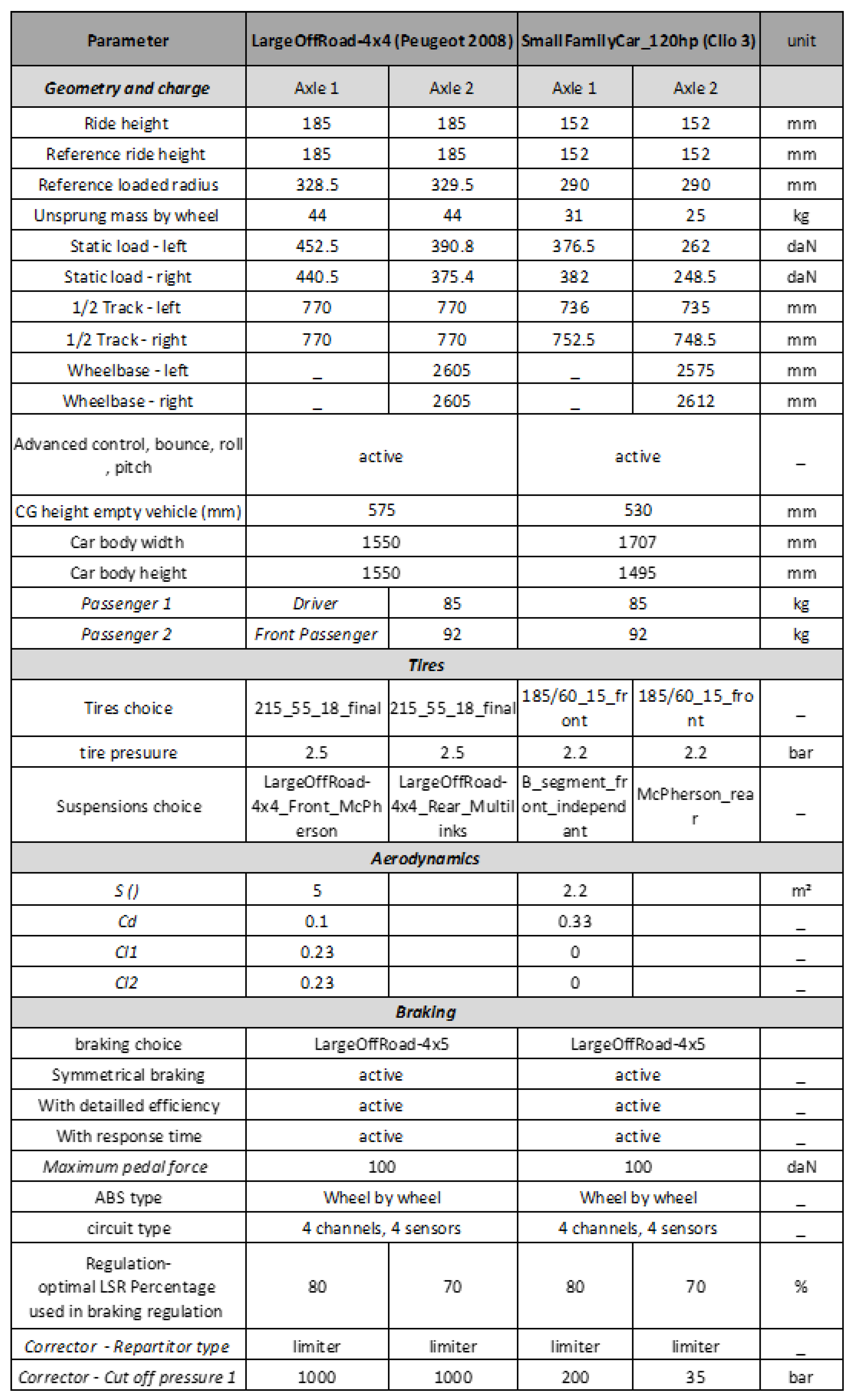
2.3. Vehicle Modeling

Modern vehicles are equipped with multiple active safety functions designed to enhance stability and control, particularly during risky maneuvers [23]. Accordingly, two vehicle models from the SCANeR 2023.3 database were selected to closely match the characteristics of the two instrumented vehicles regularly used on the designated test track. The first model, SmallFamilyCar_120, was modified to simulate an instrumented IC Renault Clio 3, while the second model, LargeOffRoad-4 × 4, was adjusted to replicate an instrumented electric Peugeot E-2008 SUV. The simulations were implemented using the “Virtual Driver (automatic)” model, which eliminates the need for a human driver by relying on an automated process to emulate driver behavior through throttle, brake, and steering commands. These inputs are managed by the “Acquisition” driver process, while the vehicle dynamics are handled by “ModelHandler”, which interfaces with the mathematical model of the vehicle. The virtual driver can be configured within the SCANeR scenario mode to control various aspects such as steering (open-loop or closed-loop), trajectory following, longitudinal control, transmission, and command data. In closed-loop mode-which we used for the simulation—the driver follows predefined paths such as straight lines, circles, or user-defined trajectories. If no speed profile is assigned, it can automatically compute a target speed using trajectory curvature and acceleration limits from the configuration file. Additionally, vehicles can be programmed to follow other vehicles with a specified time gap—positive for trailing, negative for leading. The coordinate system used in the simulation model is shown in Figure 2. To enhance accuracy, the most relevant parameters in the numerical model were modified to better align with the characteristics of the instrumented vehicles. The specific modifications are detailed in Appendix A.

2.4. Testing Maneuvers

2.4.1. Double-Lane Change Maneuver (Chicane)

The double-lane change maneuver is based on ISO 3888-1: Passenger Cars—Test Track for a Severe Lane-Change Maneuvre [24]. It involves a vehicle shifting from a 3.5 m wide lane to an adjacent lane of the same width, assuming the vehicle remains centered in the lane at all times, before returning to its original lane—simulating an overtaking maneuver to avoid an obstacle. The reference trajectory corresponds to the vehicle’s center of gravity and is maintained across different traffic speeds. The lane change occurs over a distance of approximately 20 m for light vehicles, aligning with ISO 3888-1 standards.

The objective of this simulation is to evaluate the vehicle’s handling and stability during a quick lane-change scenario, particularly in the context of avoiding an obstacle within its lane (i.e., a chicane crossing).

2.4.2. Straight-Line Emergency Braking Maneuver

The objective of this maneuver is to evaluate straight-line braking performance under the most unfavorable conditions, specifically when the car’s right-hand wheels are positioned on the metal rail. For the purpose of simulation, the ABS system was set to ‘active’ in all braking scenarios to ensure consistency in performance assessment.

2.5. Parameters of Analysis

SCANeR software provides access to over 400 parameters describing vehicle behavior. For this study, we selected the following parameters, as they are sufficient to detect various types of potential instability, including lane departure, rollover, and lateral loss of control (yaw instability):

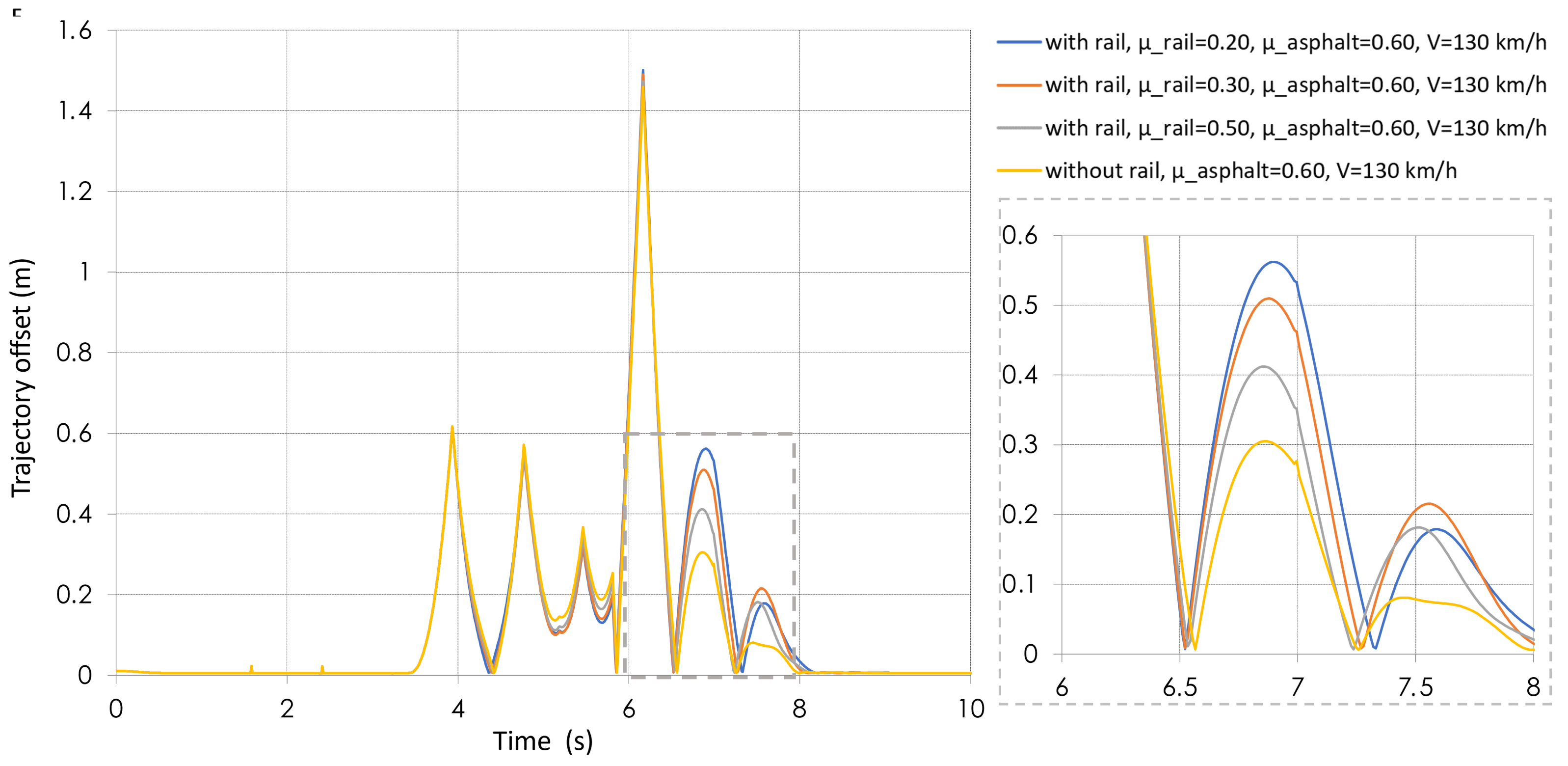
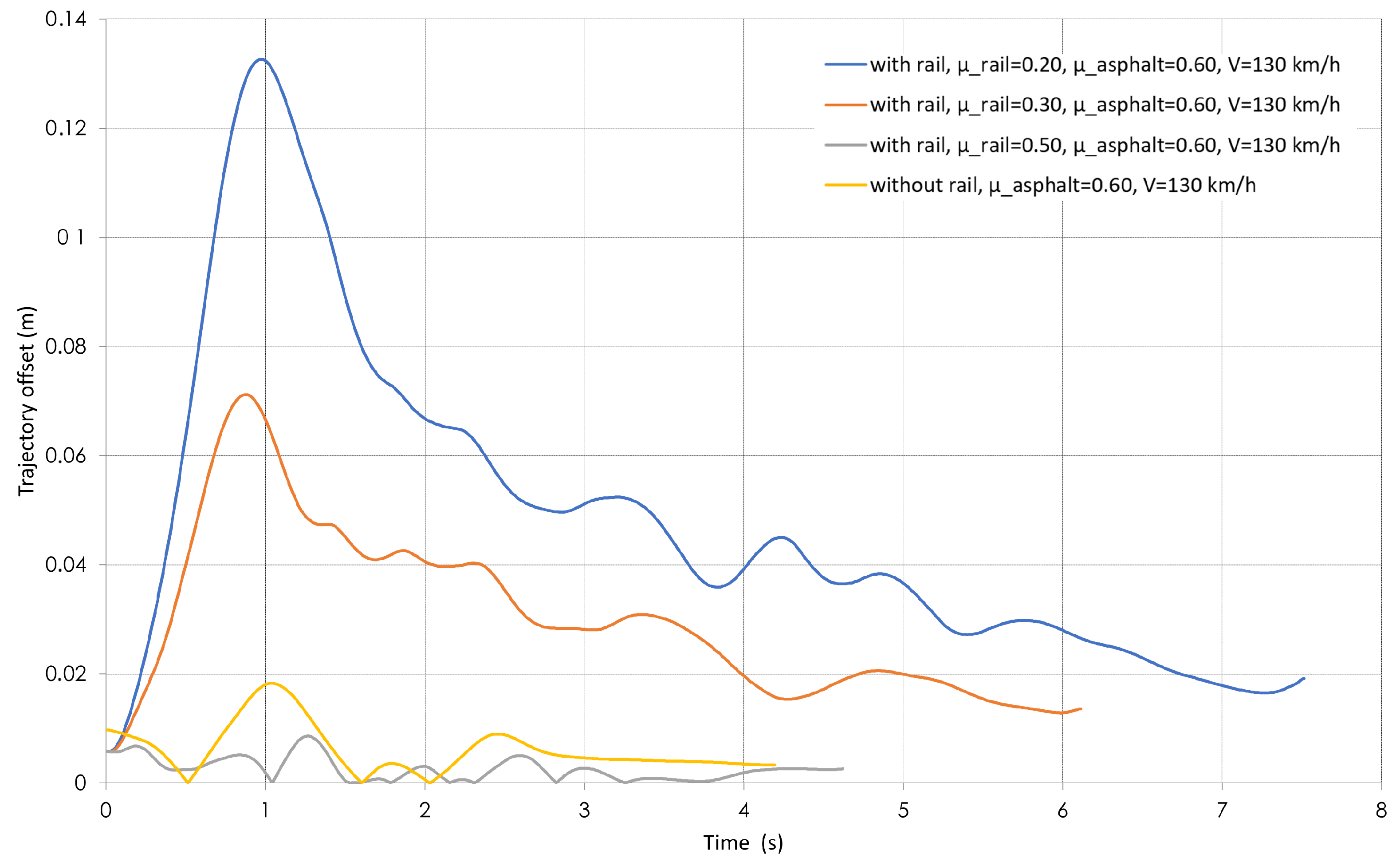
• Deviation between the target and actual trajectory, expressed in meters, is used to assess the risk of lane departure. It is calculated as the lateral distance between the vehicle’s center of gravity and the edge of the lane.
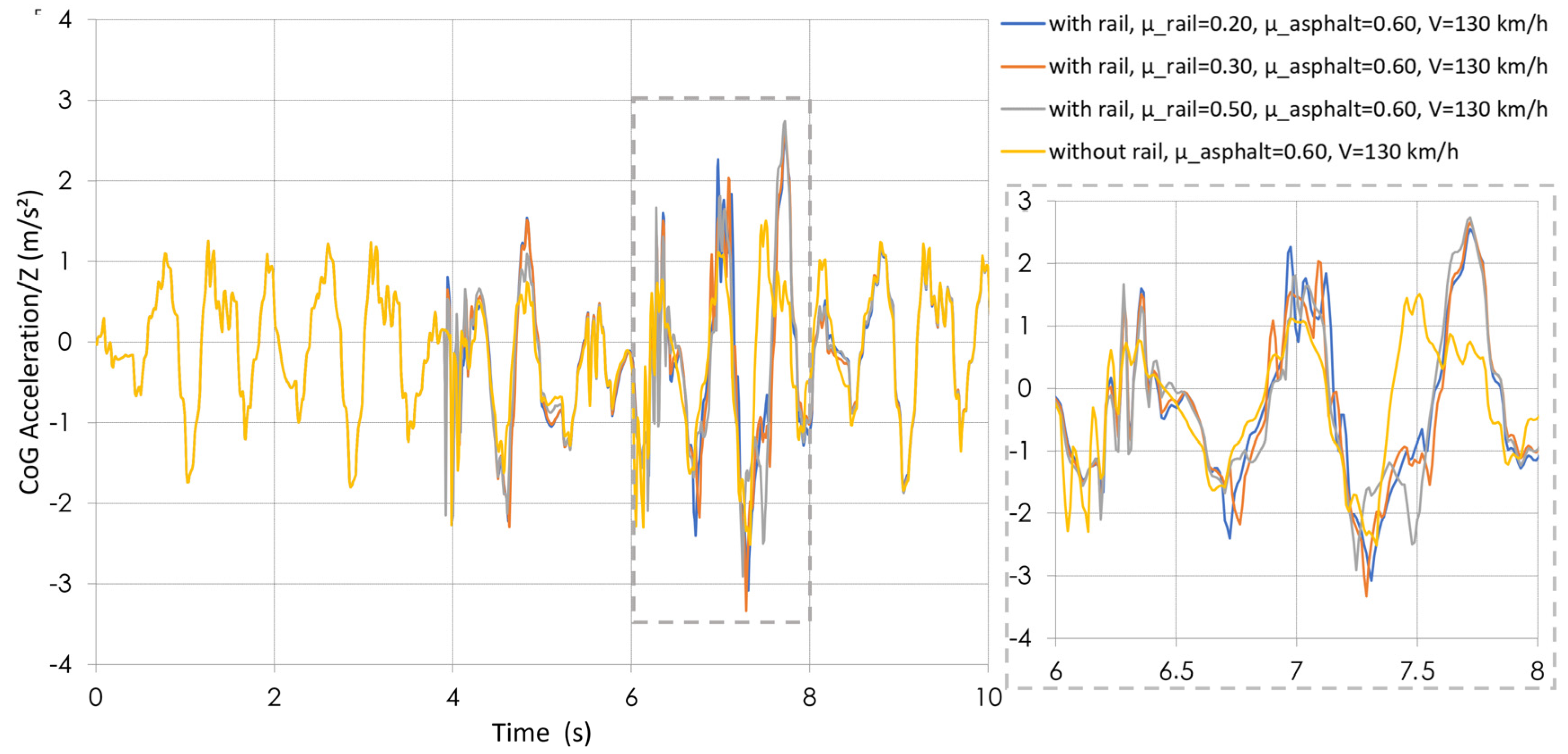
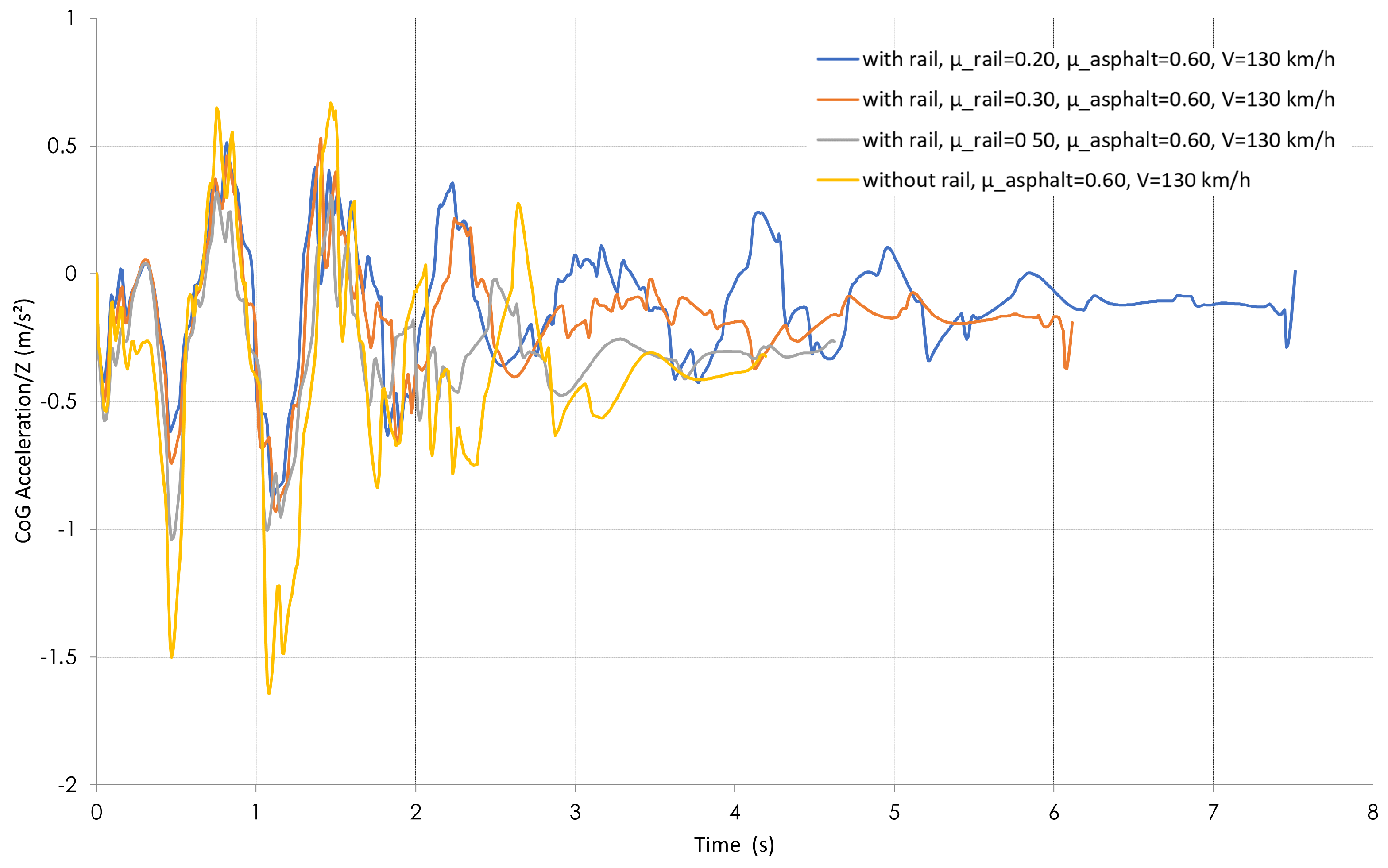
• Vertical acceleration, expressed in m/s², causes vehicle oscillations, potentially leading to discomfort and loss of control. The human body can withstand up to 50 m/s² before fainting, while in the transport sector, the usual comfort threshold is 4 m/s² [25].
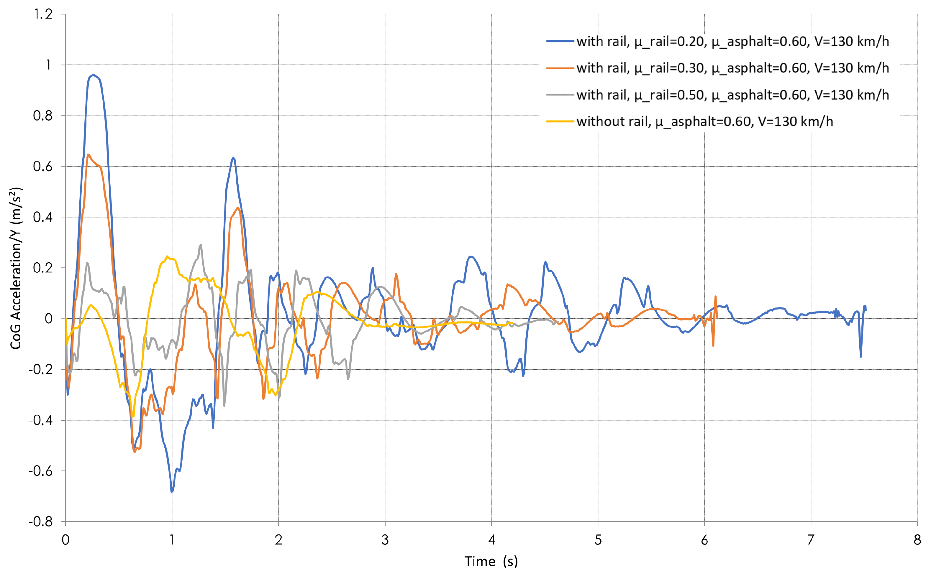
• Lateral acceleration, expressed in m/s², influences passenger comfort. Values exceeding 5 m/s² can cause discomfort to road users [25].
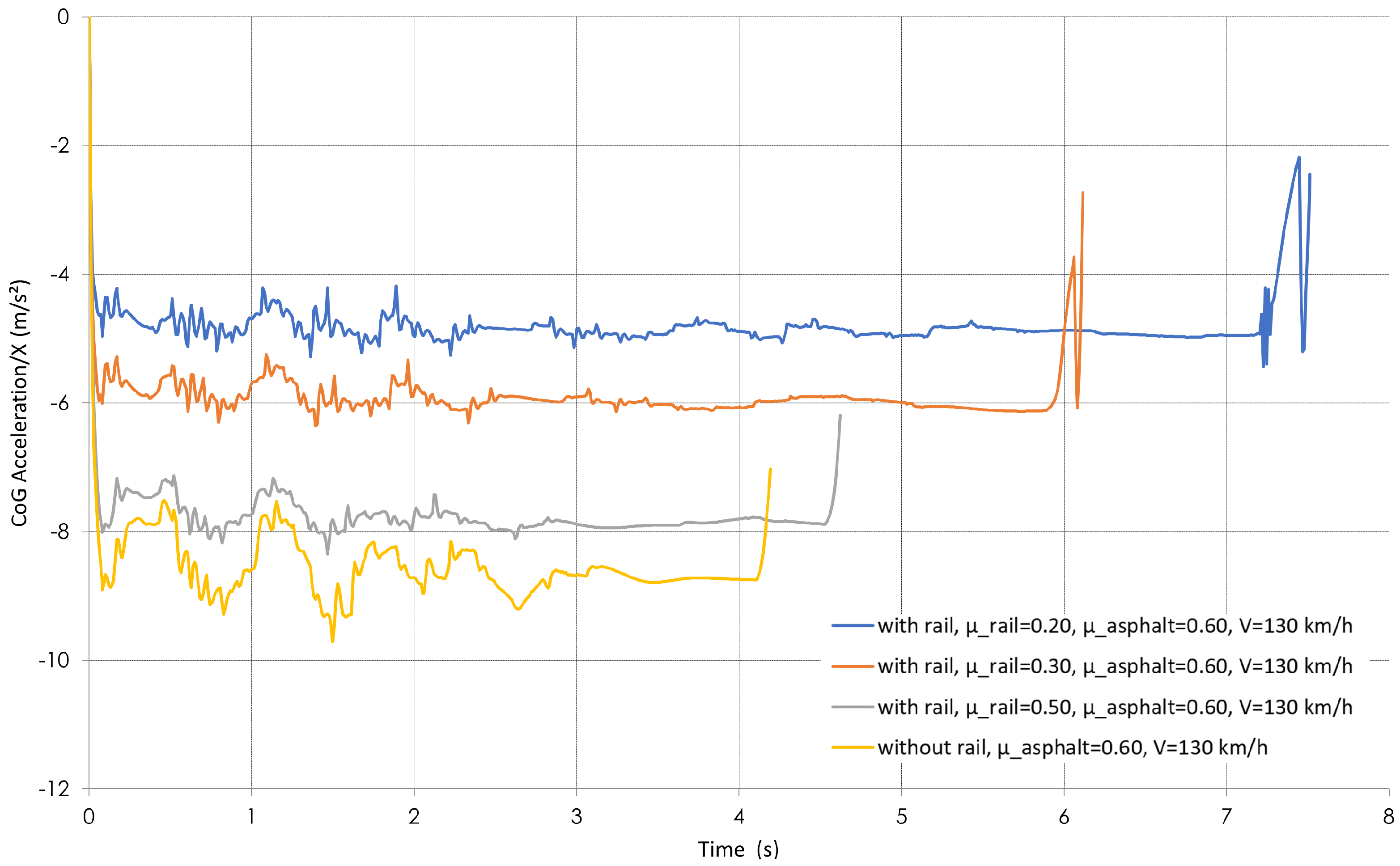
• Longitudinal acceleration, expressed in m/s², affects passenger comfort and braking performance. A comfortable acceleration is around 3 m/s², while emergency braking can reach 8–10 m/s², causing significant discomfort [26].
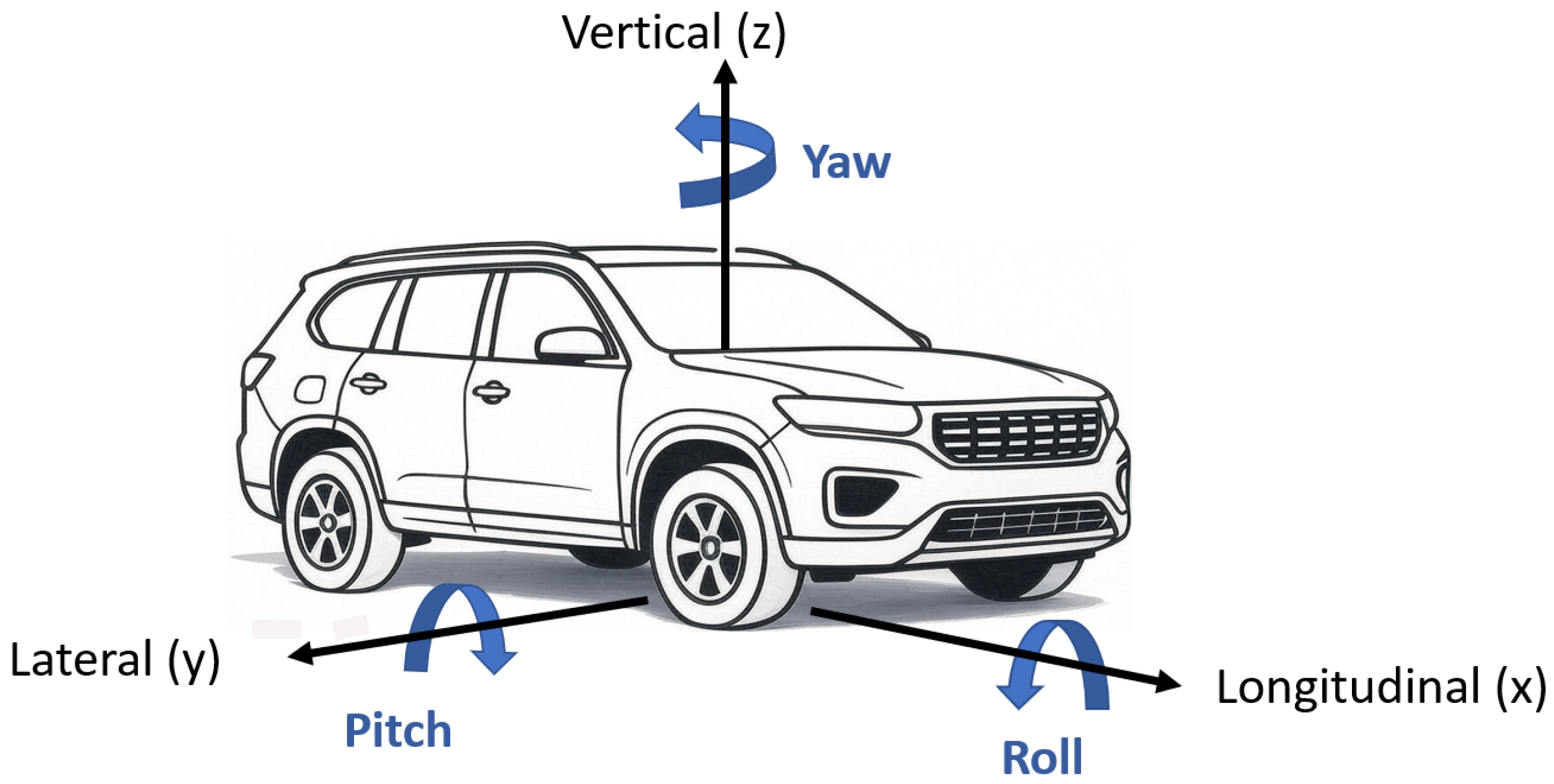
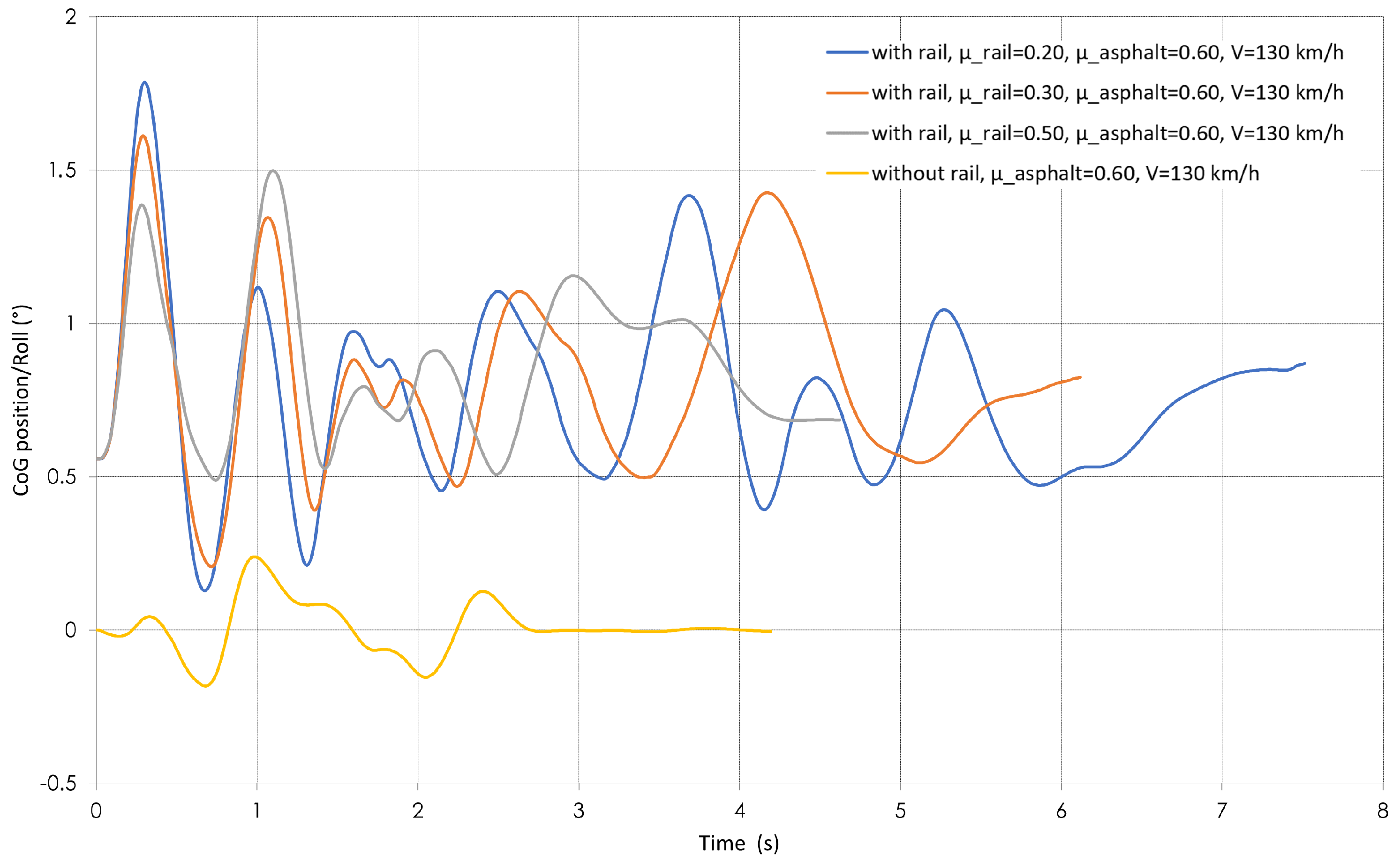
• Roll angle, expressed in degrees, describes the vehicle’s rotation around its longitudinal axis, influenced by road irregularities or centrifugal force during cornering. Roll is used to assess rollover risk. City cars typically exhibit roll angles of 2°–7°, with discomfort becoming noticeable around 7° and instability risks appearing beyond 10°–15°. However, rollover is unlikely due to their low center of gravity. SUVs, with a higher center of gravity, experience roll angles of 4°–10°, with discomfort felt at around 10° and instability risks above 15°–20°. Rollover becomes a concern at 25°–30°. Modern SUVs mitigate this risk with Electronic Stability Control (ESC) [27].
• Yaw angle, expressed in degrees, represents the vehicle’s horizontal rotation around its vertical axis. In heavy goods vehicles (HGVs), yaw is a key parameter for assessing jackknifing risk. City cars typically maintain yaw angles of 2°–5° in normal turns, with loss of control risks increasing above 10°–15°, especially in emergency maneuvers. SUVs, being taller and heavier, experience slightly higher yaw angles of 3°–7°, with instability risks rising beyond 12°–18°. Excessive yaw can lead to skidding or rollover, but ESC helps mitigate these risks [28].
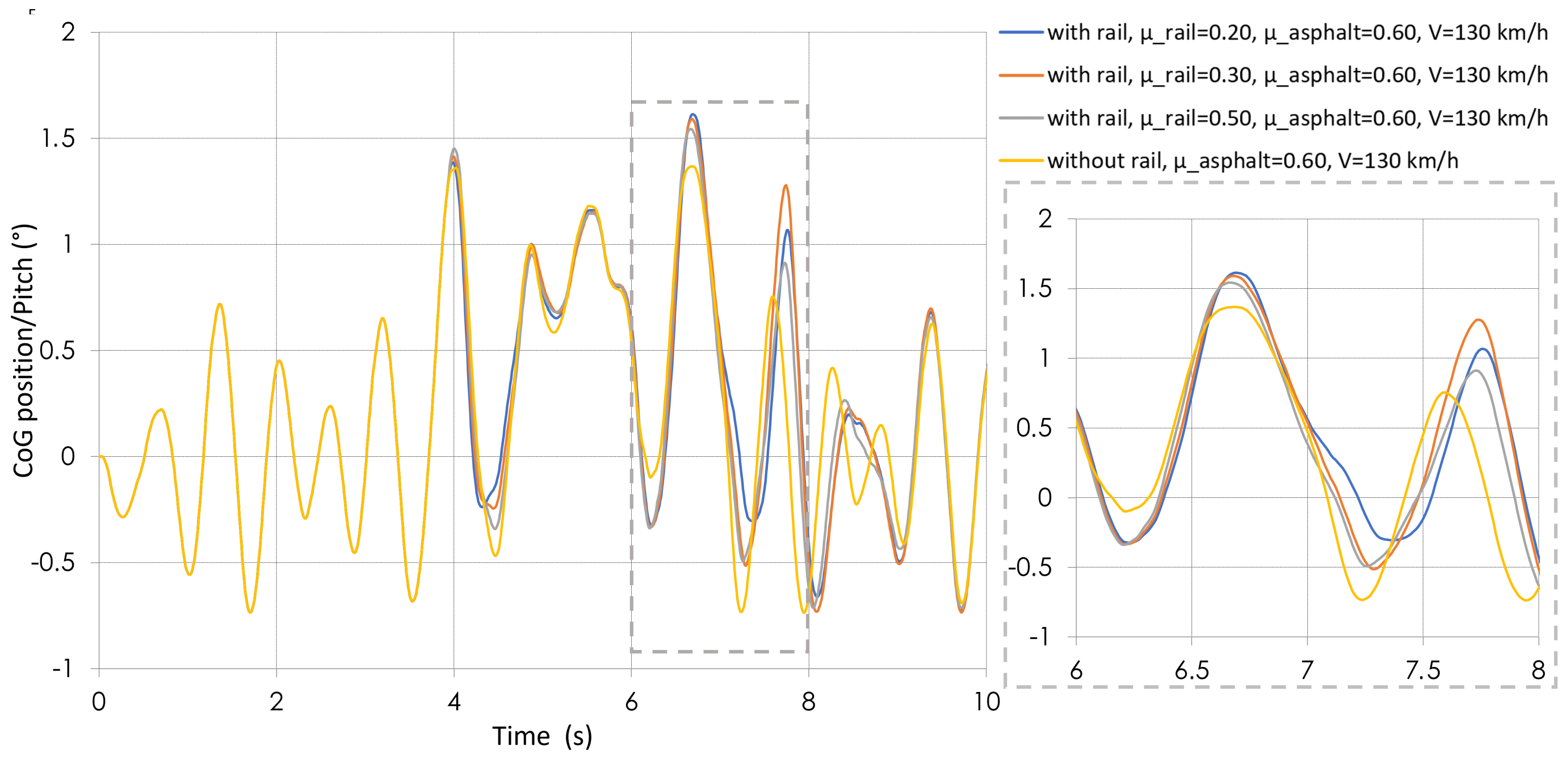
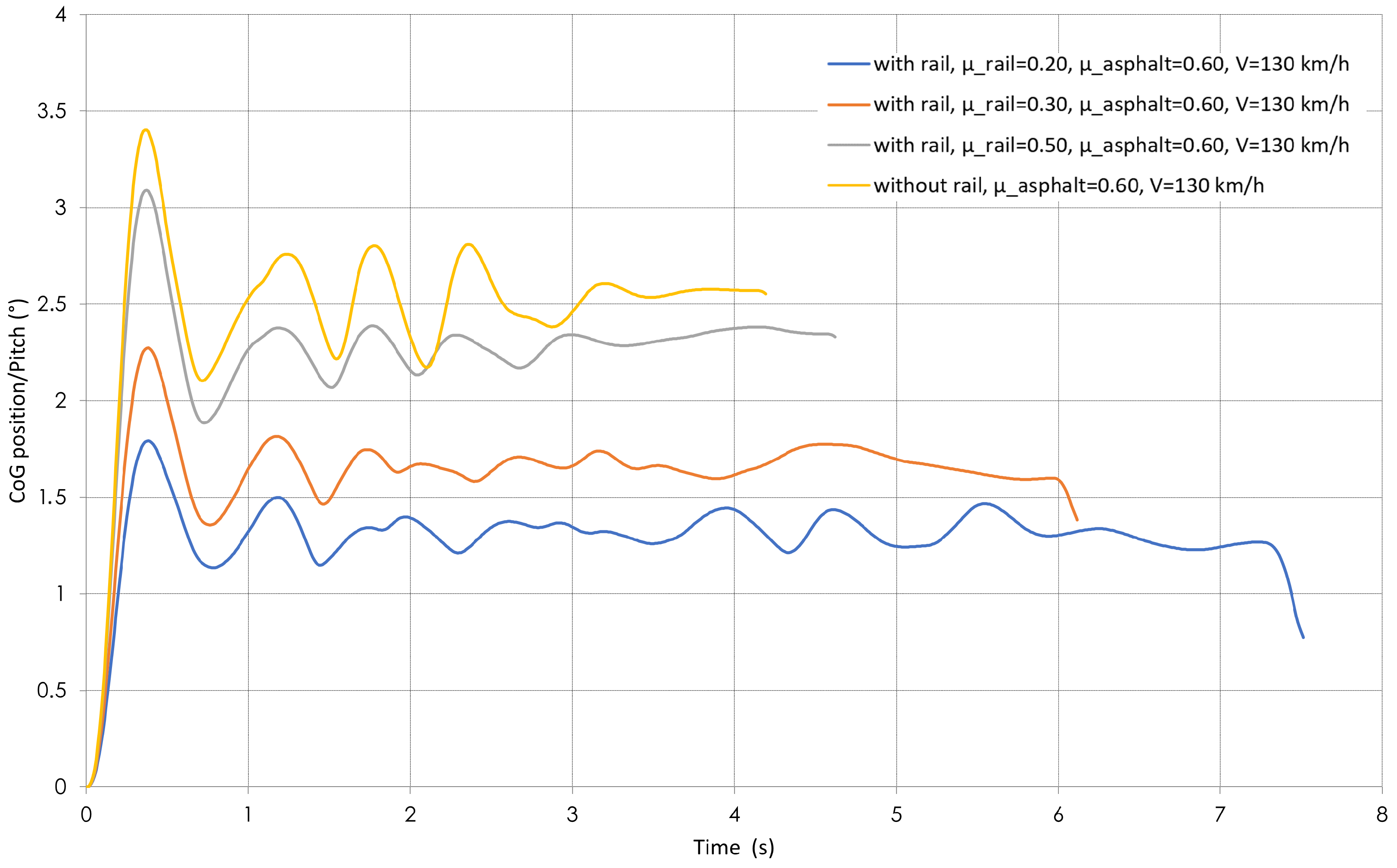
• Pitch angle, expressed in degrees, describes the rotational movement around the vehicle’s transverse axis. This oscillating movement affects ride comfort. City cars typically experience pitch angles of 1°–4° during acceleration and braking, with discomfort noticeable around 5° and potential instability beyond 10°. SUVs, due to their higher center of gravity and softer suspension, exhibit greater pitch (2°–6°), with discomfort setting in above 6° and instability risks beyond 12°. Pitch is more pronounced in SUVs during heavy braking or acceleration, particularly in off-road conditions [29].
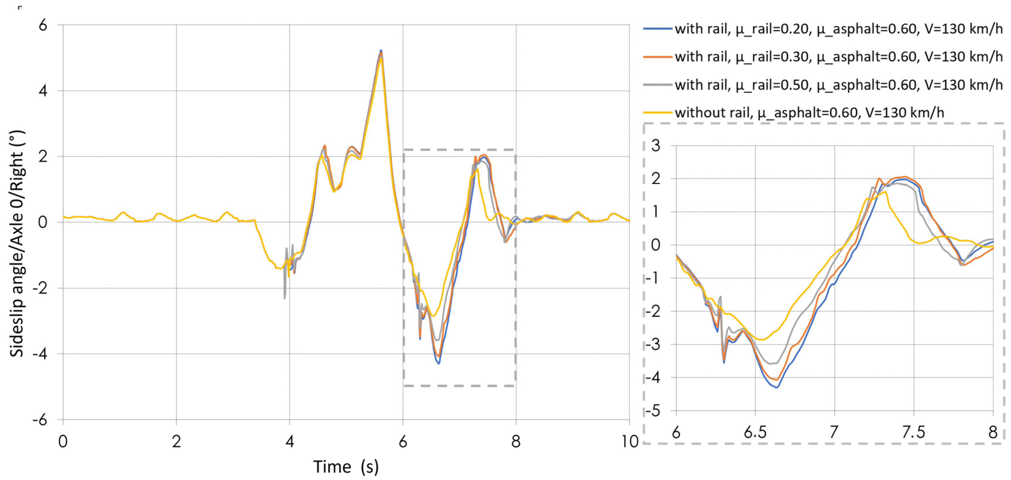
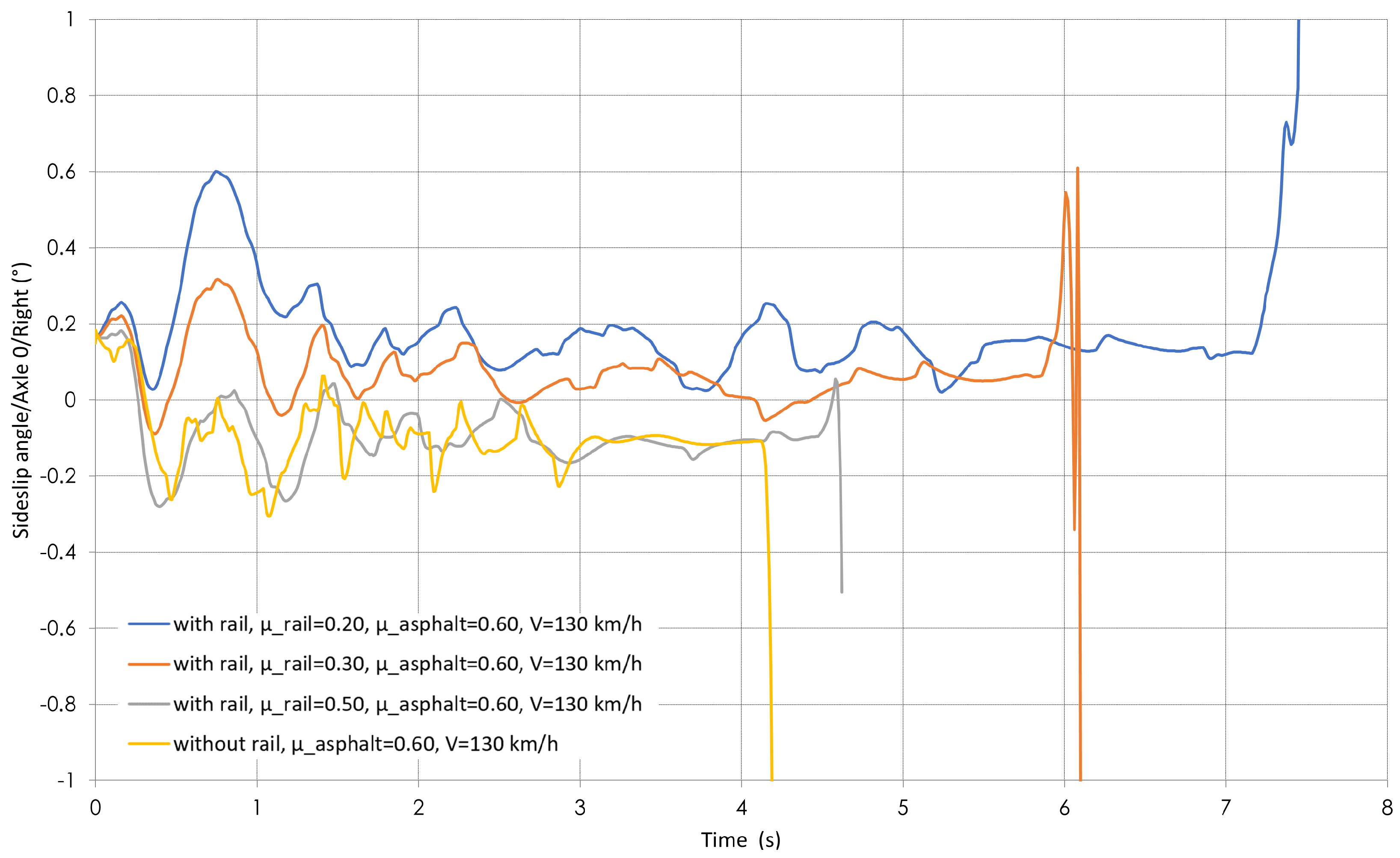
• Side slip angle, expressed in degrees, is the angle between the wheel direction and the actual trajectory of the vehicle. During cornering, this angle allows tire deformation to generate lateral forces (skid resistance). An increasing side slip angle indicates lateral instability.

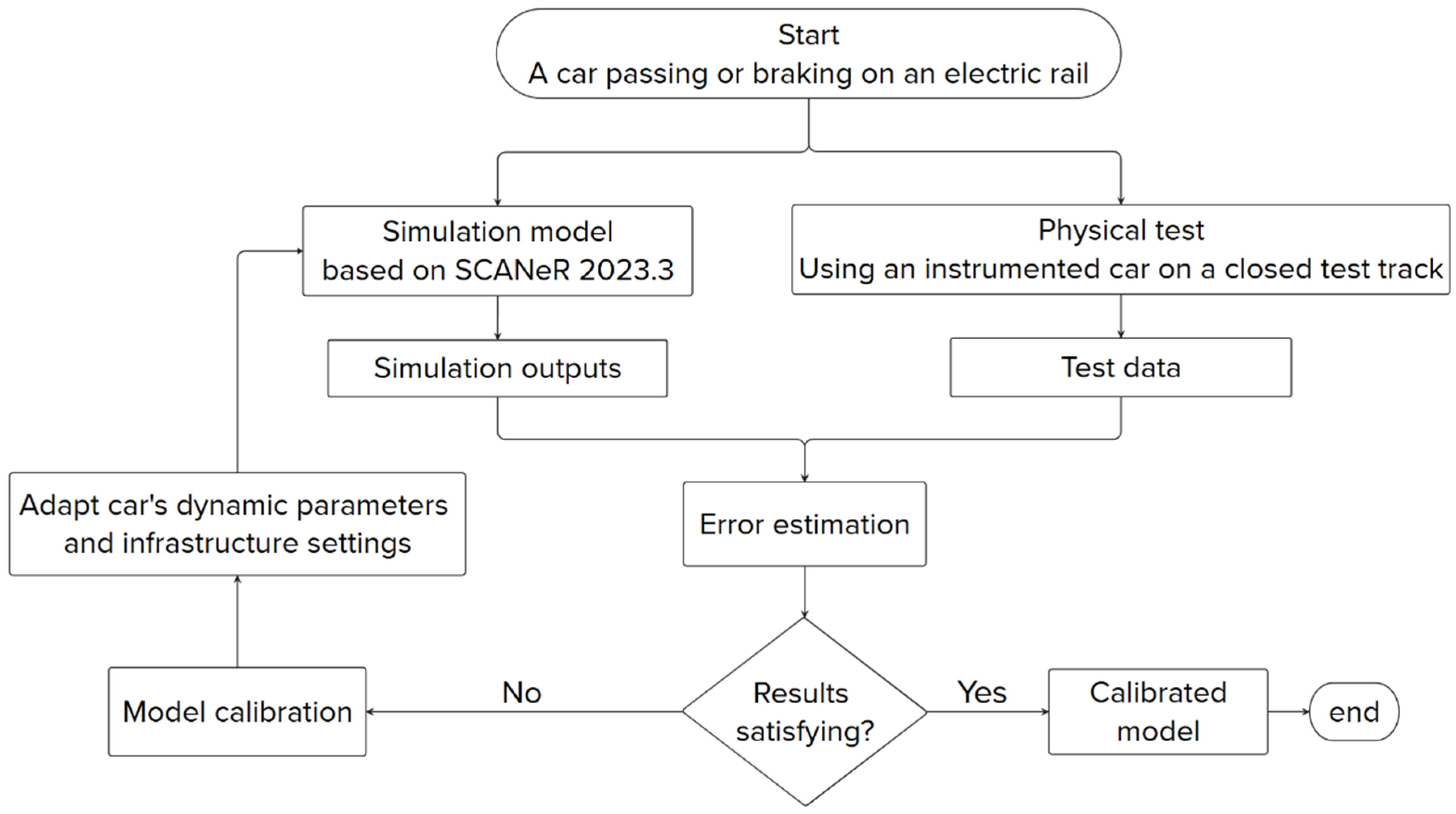
2.6. Model Calibration

To calibrate the numerical model, two instrumented passenger vehicles—a Peugeot E-2008 and a Renault Clio 3—were used. The Peugeot E-2008 GT, with a total mass of 1659.2 kg (excluding passengers), is powered by a 100 kW electric motor and equipped with Michelin Primacy 4 (215/55R18) tires. The Renault Clio 3, with a total mass of 1269 kg (excluding passengers), is powered by a 1.2 L gasoline engine and fitted with Michelin Energy Saver (185/60R15) tires.

Both vehicles were fitted with dynamometric wheels on their driven axles to precisely measure the forces and moments at the tire-road interface. In addition, laser sensors were used to determine the effective rolling radius. Each vehicle was also equipped with an Inertial Measurement Unit (IMU) capable of measuring acceleration in the x, y, and z directions, as well as pitch, roll, and yaw, a Global Positioning System (GPS) device, and a speed sensor to capture comprehensive motion data.

An experienced driver conducted double-lane change and braking maneuvers at various speeds on a representative pavement surface with a Sideforce Friction Coefficient (SFC) of 0.60. The tests were conducted on a closed test track located at the university site in Nantes.

The data recorded by the onboard sensors were systematically compared with the outputs of the numerical simulations. Discrepancies between measured and simulated data were analyzed, and the numerical model were iteratively refined and calibrated to improve alignment with the experimental results. We used a trial-and-error method to minimize the error between the measured and simulated values. The calibration process was stopped once the error reached a minimal value, as shown in Figure 3.

Figure 4 presents a comparison between simulated and experimental braking distances for an SUV at different velocities (70, 90, 110, and 130 km/h). The results show a close agreement between the two datasets, particularly at higher speeds. At lower speeds (70 km/h, 90 km/h and 110 km/h), the experimental values are slightly higher than the simulated ones, whereas at 130 km/h, the differences are minimal. This shows that the simulation results are very close to experimental data, with a minimum percentage of error of 0% and a maximum percentage of error of around 3.48%. This comparison serves to calibrate the mathematical model by validating the accuracy of the simulation in predicting real-world braking performance. The slight variations between the two datasets could be attributed to factors such as unevenness of road profile, braking system efficiency, or environmental conditions during testing. Overall, the figure demonstrates that the mathematical model provides a reliable approximation of the SUV’s braking behavior.

Figure 5 presents a comparison between lateral acceleration data obtained from the simulation and real-world track measurements conducted during a controlled double-lane change maneuver with an SUV. The test was conducted on a dry asphalt surface with a skid resistance coefficient (SFC) of 0.60, and the vehicle speed was maintained at 90 km/h. The lateral acceleration data was captured using onboard sensors and simulation outputs under identical test conditions. Over time, both curves exhibit similar trends, with noticeable peaks and oscillations, indicating comparable vehicle dynamics in both cases. However, some discrepancies are observed, particularly in peak acceleration values and certain transient responses. The calculated percentage error (average deviation between the two curves) is 5.89%. Additionally, the wave amplitude (peak-to-peak lateral acceleration) is 11.3 m/s² in the simulation and 12.6 m/s² in the experimental data. These differences are likely due to real-world uncertainties such as driver behavior, suspension effects, or sensor noise.

At 70 km/h, the maximum simulated acceleration is 4.6 m/s², while the experimental value is slightly higher at 4.8 m/s². At 90 km/h, the maximum simulated acceleration reaches 6.6 m/s², whereas the experimental measurement is slightly lower at 6.25 m/s².

The remaining analysis parameters were also compared to support the calibration of the simulation model. However, to avoid overloading the article with figures, we included only two key parameters—braking distance and lateral acceleration—in the manuscript. For the other parameters, the error between the simulation and the physical test results ranges from 3% to 10%.

The close agreement between simulation and experimental results suggests that the numerical model accurately represents the SUV’s lateral dynamics, making it well-suited for further calibration and validation.

3. Simulation Results—Double-Lane Change Maneuver

Simulations were implemented for two types of vehicles (SUV and city car) across 20 configurations (5 speeds, combined with one configuration without the rail and three configurations with different skid resistance levels for the ERS system). Simulation results for accelerations (longitudinal, lateral, vertical) and angular positions (roll, pitch, yaw, side-slip angle) are presented; however, to avoid overloading the paper with graphs and given the similar simulation behavior observed between the SUV and the city car, the output graphs for the city car will be omitted. Instead, the graphs of the SUV at the maximum testing speed of 130 km/h will be presented and a concise summary of the outputs of the city car will be provided.

3.1. Trajectory Deviation

The trajectory deviation of the center of gravity from the reference trajectory of the SUV is illustrated in Figure 6. The results show that variations in the ERS skid resistance do not induce any significant trajectory deviations, regardless of the speed considered.

This deviation is then compared to the existing clearance between the edge of the vehicle and the lane boundary to ensure that the vehicle remains within the left traffic lane during the maneuver. The SUV is equipped with 215/55R18 tires, and the distance from the vehicle’s centerline to the outer edge of the tire is 0.775 m. When the vehicle is centered in the lane, the distance from the outer edge of the tire to the lane boundary is 0.975 m. The maximum observed trajectory deviation is 0.25 m, which is smaller than this clearance, confirming that the vehicle remains entirely within the traffic lane throughout the lane-change maneuver. Similarly, the city car demonstrates comparable behavior, with a maximum trajectory deviation of 0.20 m at a speed of 130 km/h.

3.2. Vertical Acceleration

Vertical accelerations at the vehicle’s center of gravity remain low, regardless of the ERS skid resistance level or the speed of the lane-change maneuver (Figure 7). Across all configurations tested, vertical accelerations stay below 3.0 m/s² in absolute terms. Peak values of approximately 2.0 m/s² are observed during the moments when the driver initiates steering to change direction. Outside these peaks, acceleration values remain consistently below 1.0 m/s².

These results comply with the ISO 22179 standard for adaptive cruise control systems, which specifies acceleration limits ranging from +4/−5 m/s² at 20 m/s to +2/−3.5 m/s² at 5 m/s [25].

A slight reduction in vertical acceleration is observed each time one of the right-hand wheels crosses the rail. This variation is particularly noticeable (around 7.3 m/s²) for low skid resistance levels (SFC = 0.35) across all tested speeds (70, 90, 110, and 130 km/h). In other scenarios, the variation in vertical acceleration remains below 0.5 m/s², with minimal impact on vehicle dynamics. These results indicate that the ERS system introduces a minor increase in driving discomfort under conditions of low skid resistance (SFC = 0.20), in addition to the discomfort caused by the lane-change maneuver itself.

Similarly, the vertical accelerations at the city car’s center of gravity remain low, irrespective of the skid resistance level of the ERS system or the speed of the lane-change maneuver. For all tested configurations, vertical accelerations do not exceed 3.0 m/s² in absolute value. Peaks of around 2.0 m/s² occur during the initial steering to initiate the lane change, while outside these peaks, acceleration values consistently remain below 1.0 m/s².

3.3. Lateral Acceleration

Lateral accelerations at the vehicle’s center of gravity are presented in Figure 8. Analysis of the graphs indicates that acceleration values remain below the 5.5 m/s² threshold at 70 km/h. At 90 km/h, maximum values reach approximately 7.5 m/s², and at 130 km/h, they approach 10 m/s². These values suggest a moderate level of driving discomfort during the lane-change maneuver.

The city car shows similar behavior with a moderate level of discomfort at 130 km/h during the lane-change maneuver.

3.4. Longitudinal Acceleration

Longitudinal acceleration variations are shown in Figure 9 for three ERS skid resistance levels. Acceleration values for both the SUV and the city car are below 0.4 m/s², which is ten times lower than the discomfort threshold.

3.5. Roll Angle

Figure 10 illustrates the variations in roll angle for the SUV across three skid resistance levels of the ERS system. The roll angles remain below 5°, indicating minimal vehicle roll and no risk of rollover. A slight increase in roll angle is observed at low skid resistance levels (SFC = 0.20) and high speeds (90, 110 and 130 km/h), but this variation is negligible and does not affect vehicle stability.

Similarly, for the city car, roll angle values also remain below 5°, confirming minimal rolling movement and no risk of overturning.

3.6. Yaw Angle

Figure 11 illustrates the variations in yaw angle for the SUV across three skid resistance levels of the ERS system. The yaw angle increases up to 8°, which is expected due to the lane-change maneuver. No observable effect of the ERS system on the yaw angle is detected in the numerical simulations. Similar behavior is observed for the city car.

3.7. Pitch Angle

Figure 12 shows the variations in pitch angle for the SUV across three skid resistance levels of the ERS system. The pitch angle increases up to 1.5°, which is attributed to the lane-change maneuver. The ERS system crossing has no observable effect on the pitch angle in the numerical simulations. A similar behavior is observed for the city car.

3.8. Side Slip Angle

Figure 13 shows the evolution of the side slip angle for the front right (Axle 0) and rear right (Axle 1) tires across three ERS skid resistance levels and three rail crossing speeds. All three graphs reveal very slight variations in the side slip angle (approximately 0.5° in absolute value), regardless of the configuration. This indicates that the tires experience only minimal deformation as the ERS system passes over them, with no noticeable impact on vehicle dynamics during the lane-change maneuver. A similar behavior is observed for the city car.

4. Simulation Results-Emergency Braking

Simulations were implemented under the same conditions as the double-lane change maneuver. The results are presented below:

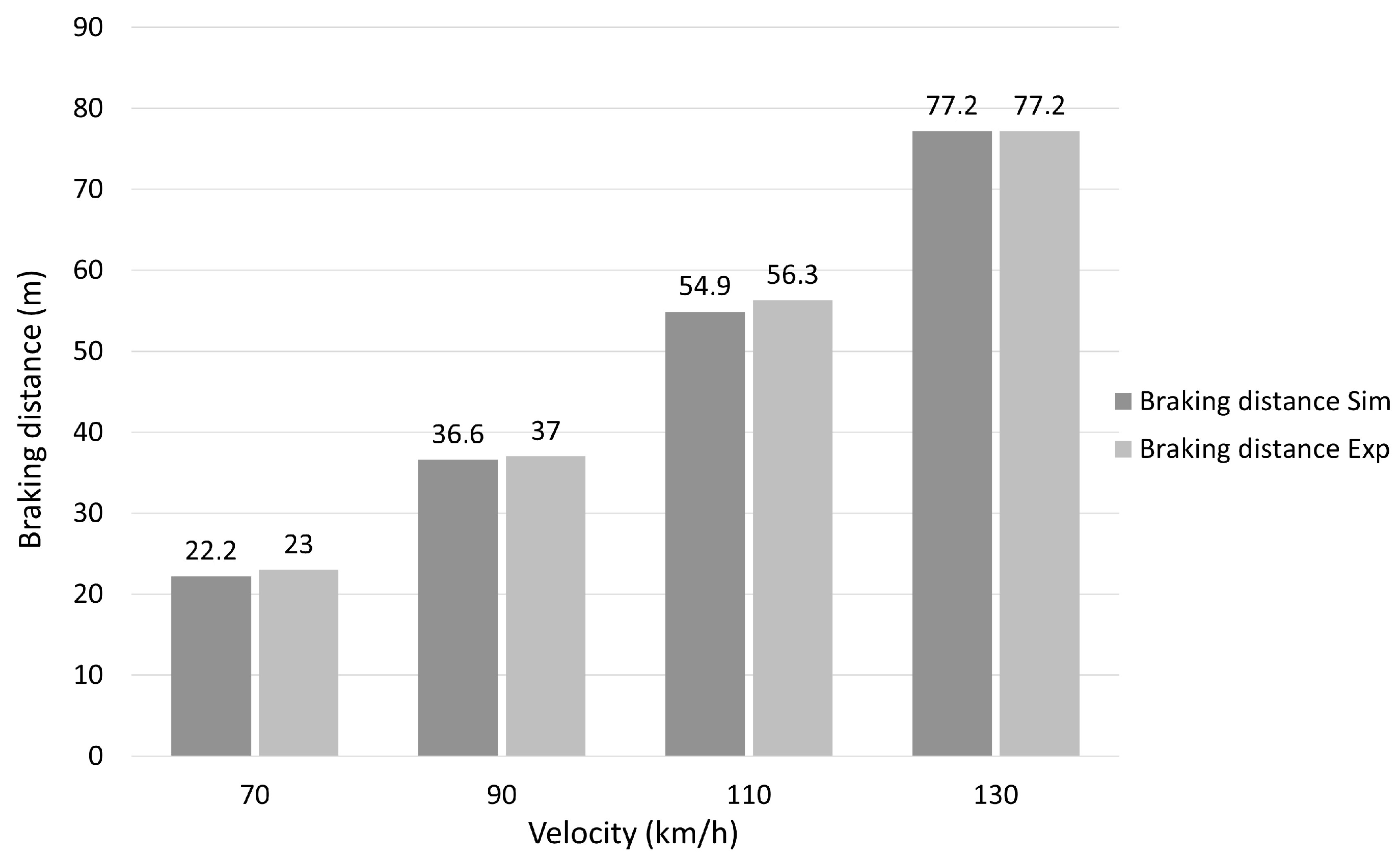
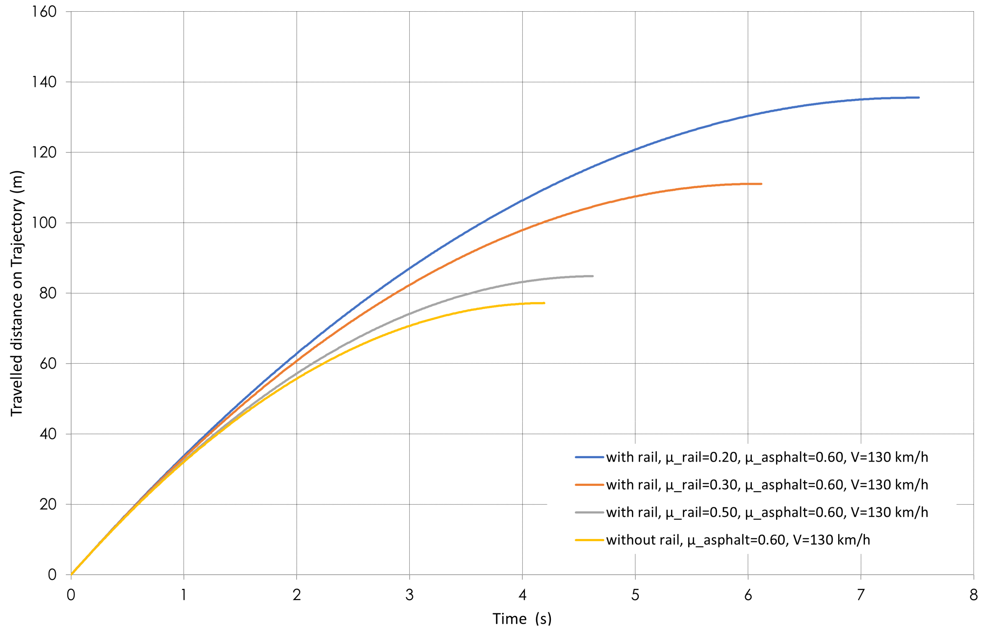
4.1. Braking Distance

The distance traveled as a function of time during the braking maneuver for the SUV is shown in Figure 14 for all test speeds. Variations in the skid resistance of the ERS rail lead to a significant increase in braking distance, disproportionate to the skid resistance level. In other words, a reduction in skid resistance causes an exaggerated increase in braking distance, making the braking system less effective compared to a scenario without the rail.

Table 1. Simulated braking distance as a function of skid resistance level and speed.

	Braking Distance (m)
SCF	70 km/h	90 km/h	110 km/h	130 km/h
0.2	39.3	64.8	96.8	135.6
0.3	23.4	52.9	79.2	111.1
0.5	24.4	40.3	60.4	84.9
0.6	22.2	36.6	54.9	77.2

presents the simulated braking distances as a function of two key variables: skid resistance level of the ERS system (ranging from 0.2 to 0.6) and speed (70, 90, 110, and 130 km/h). The table indicates that braking distances increase as the skid resistance level decreases for a given speed. This increase in braking distance poses a significant risk of collision in the event of emergency braking, highlighting the potential danger associated with reduced skid resistance. The simulation results of the city car show similar behavior.

For road design in France, the Stopping Sight Distance (SSD) for highways (130 km/h) is approximately 265 m under standard conditions. As the simulation does not include the Perception-Reaction Distance, the braking distance is 193.1 m [30], comparing the results of simulations with this value shows that all braking distances are safe for all configurations.

4.2. Trajectory Deviation

The deviation of the trajectory of the center of gravity of the SUV compared to the reference trajectory is shown in Figure 15 at 130 km/h. It can be observed that the variation in skid resistance of the ERS system does not cause a significant deviation in the trajectory, regardless of the speed considered. The measured deviation, approximately 10 cm, indicates the absence of loss of control during braking on the rail. Similarly, the deviation measured for the city car does not exceed 10 cm, further demonstrating the lack of loss of control when braking on the rail.

4.3. Vertical Acceleration

Vertical accelerations at the SUV’s center of gravity remain low regardless of the ERS skid resistance level and the braking maneuver execution speed (Figure 16). Vertical accelerations are below 1.0 m/s² in absolute value for all configurations tested. A similar trend is observed for the city car.

4.4. Lateral Acceleration

Lateral accelerations at the SUV center of gravity are shown in Figure 17 for three ERS system skid resistance levels. Analysis of the graphs shows that lateral acceleration values remain below the threshold at 1.0 m/s² in absolute value for all tested configurations, which indicates no loss of control or driving discomfort. A similar behavior is observed for the city car.

4.5. Longitudinal Acceleration

Variations in longitudinal acceleration are shown in Figure 18 for three ERS skid resistance levels. Note that as the resistance to skidding decreases, the vehicle loses traction and acceleration decreases accordingly. The graph illustrates the importance of rail skid resistance in maintaining controlled deceleration, particularly at high speeds, and shows that the ERS system plays a crucial role in braking stability.

For the city car, it is noted that the more skid resistance decreases, the more the vehicle loses traction, and acceleration decreases accordingly.

4.6. Roll Angle

Figure 19 illustrates the variations in roll angle for three levels of ERS skid resistance. The recorded values remain below 2°, indicating minimal vehicle roll and no risk of rollover. While the graph shows a slight fluctuation in roll angle as the ERS system is engaged, this variation is negligible.

For the city car, the recorded values also remain below 2°, indicating minimal rolling movement and no risk of overturning.

4.7. Yaw Angle

Figure 20 illustrates the variations in the yaw angle for three levels of ERS skid resistance. The yaw angle reaches 0.8° when the vehicle brakes on the rail with the lowest skid resistance level (0.20), however, this does not impact the lateral stability of the car.

For the city car, the yaw angle also increases to 0.8° under the same braking conditions on the rail with an skid resistance level of 0.20.

4.8. Pitch Angle

Figure 21 illustrates the variations in pitch angle for three skid resistance levels of the ERS system. The curves show that the pitch angle is strongly influenced by rail skid resistance. Lower skid resistance results in a smaller pitch amplitude, particularly in the initial seconds of braking. The initial oscillations reflect the vehicle’s dynamic response to changes in skid resistance, whereas the absence of a rail leads to significantly larger pitch amplitudes.

In contrast, higher skid resistance reduces these oscillations and stabilizes the pitch more quickly, enhancing vehicle control. Without a rail, the maximum pitch angle reaches 3.5° at the moment of braking. With a rail, the pitch angle becomes more pronounced at high skid resistance due to increased friction forces, which generate greater front-to-rear load transfer. However, this pitching effect is quickly absorbed by the vehicle’s suspension system, allowing for rapid stabilization. The city car shows similar behavior.

4.9. Side Slip Angle

Figure 22 illustrates the evolution of the side slip angle of the right front tires (Axle 0) for three levels of ERS system skid resistance and four braking speeds. Across all four graphs, the side slip angle shows only minimal variations (approximately 0.5° in absolute value), regardless of the configuration considered. This suggests that the tires experience slight deformation as the ERS system passes but that it has no significant impact on the braking maneuver.

For the city car, the same small variations in the side slip angle (approximately 0.5° in absolute value) are observed in all configurations. This confirms that the tires undergo slight deformation when the ERS system passes, without any notable effect on braking performance.

5. Conclusions

Simulations of double-lane change (chicane) and emergency braking maneuvers were implemented to evaluate the impact of the conductive ERS system on vehicle dynamics. The double-lane change tests were carried out on both an SUV and a city car in 20 different configurations, combining 4 levels of skid resistance and 5 speeds. The results showed no significant effect of the ERS system on vehicle dynamics. The roll, yaw, and side slip angles were minimal. Additionally, trajectory deviations remained within the available lane space (<0.25 m, with no recorded lane departures), and vertical and horizontal acceleration levels did not exceed discomfort thresholds. Acceleration variations remained limited when crossing the ERS system.

Emergency braking simulations were also implemented to assess the impact of the conductive ERS system on vehicle stopping distances. These tests were conducted on both an SUV and a city car across 20 different configurations, combining 4 skid resistance levels and 5 speeds. The results revealed a significant impact of the ERS system on emergency braking distance. When braking with the left wheel on asphalt and the right wheel on the rail, the braking distance increased due to the reduced skid resistance coefficient of the rail, potentially increasing the risk of loss of control during emergency braking. The roll, yaw, pitch, and side slip angles were minimally or not affected by the ERS system. Trajectory deviations remained within the available lane space (<0.15 m, with no recorded road departures), and vertical and horizontal acceleration levels did not exceed discomfort thresholds. Finally, while longitudinal deceleration increased sharply during braking, it decreased as the rail’s skid resistance coefficient decreased. Vertical and lateral accelerations remained relatively stable when crossing the ERS system.

It is important to note that these simulations were implemented under highly unfavorable conditions, with non-rounded rail profiles and a non-deformable system, which tend to amplify acceleration values. In future work, a dedicated test track will be constructed to conduct experiments that assess the impact of the electric rail on vehicle dynamics in real-life situations. The experimental results will then be compared with simulation outcomes to validate the developed model.

References

1. Yu, X.; LeBlanc, S.; Sandhu, N.; Wang, L.; Wang, M.; Zheng, M. Decarbonization potential of future sustainable propulsion—A review of road transportation. Energy Sci. Eng. 2024, 12, 438–455. [Google Scholar] [CrossRef]
2. Lacire, S.; Hauet, J.-P. La Route éLectrique: Il Faut s’y préParer; Équilibre des Énergies: Paris, France, 2023. [Google Scholar]
3. Des Routes éLectriques (ERS) Pour Contribuer à déCarboner le Transport Routier, Rapport du GT1: Intérêt des Solutions et Conditions de RéUssite; Ministère de la Transition Écologique: Paris, France, 2021.
4. Bateman, D.; Leal, D.; Reeves, S.; Emre, M.; Stark, L.; Ognissanto, F.; Myers, R.; Lamb, M. Electric Road Systems: A Solution for the Future? 2018SP04EN; World Road Association: La Défense, France, 2018. [Google Scholar]
5. Swedish, I.V. Slide-In Electric Road System-Inductive Project Report; Viktoria Swedish ICT: Gothenburg, Sweden, 2014. [Google Scholar]
6. Rajamani, R. Vehicle Dynamics and Control; Springer Science and Business Media: Berlin/Heidelberg, Germany, 2011. [Google Scholar]
7. Magel, E.; Tajaddini, A.; Trosino, M.; Kalousek, J. Traction, forces, wheel climb and damage in high-speed railway operations. Wear 2008, 265, 1446–1451. [Google Scholar] [CrossRef]
8. Olofsson, U.; Sundvall, K. Influence of leaf, humidity and applied lubrication on friction in the wheel-rail contact: Pin-on-disc experiments. Proc. Inst. Mech. Eng. Part F J. Rail Rapid Transit 2004, 218, 235–242. [Google Scholar] [CrossRef]
9. Rong, K.-J.; Xiao, Y.-L.; Shen, M.-X.; Zhao, H.-P.; Wang, W.-J.; Xiong, G.-Y. Influence of ambient humidity on the adhesion and damage behavior of wheel–rail interface under hot weather condition. Wear 2021, 486, 204091. [Google Scholar] [CrossRef]
10. Meymand, S.Z.; Keylin, A.; Ahmadian, M. A survey of wheel–rail contact models for rail vehicles. Veh. Syst. Dyn. 2016, 54, 386–428. [Google Scholar] [CrossRef]
11. He, J.; Xiang, H.; Li, Y.; Han, B. Aerodynamic performance of traveling road vehicles on a single-level rail-cum-road bridge under crosswind and aerodynamic impact of traveling trains. Eng. Appl. Comput. Fluid Mech. 2022, 16, 335–358. [Google Scholar] [CrossRef]
12. Gupta, A.; Pradhan, S.K.; Bajpai, L.; Jain, V. Numerical analysis of rubber tire/rail contact behavior in road cum rail vehicle under different inflation pressure values using finite element method. Mater. Today Proc. 2021, 47, 6628–6635. [Google Scholar] [CrossRef]
13. Müller, S.; Blundell, M. The testing of pneumatic tyres for the interpretation of tyre behaviour for road/rail vehicles when operating on rails. Proc. Inst. Mech. Eng. Part J. Automob. Eng. 2023, 237, 3275–3284. [Google Scholar] [CrossRef]
14. Chou, C.-P.; Lee, N. Skid resistance of manhole covers: Current situation in Taiwan. In Proceedings of the Eastern Asia Society for Transportation Studies Vol. 8, the 9th International Conference of Eastern Asia Society for Transportation Studies, Jeju, Republic of Korea, 20–23 June 2011; Eastern Asia Society for Transportation Studies: Kawana, Japan, 2011; p. 12. [Google Scholar]
15. Huang, C. Evaluation of Skid Resistance of Pattern Design for Manhole Cover. Ph.D. Thesis, National Taiwan University, Taiwan, China, 2010. [Google Scholar]
16. Chou, C.-P.; Huang, C.-K.; Chen, A.; Tsai, C.Y. Pattern design of manhole cover and its influence on skid resistance. Int. J. Pavement Res. Technol. 2013, 6, 351. [Google Scholar]
17. Avsimulation Website. Available online: https://www.avsimulation.com/scaner-catalog/?lang=fr (accessed on 15 May 2024).
18. Guo, C. Conception des Principes de Coopération Conducteur-véhicule Pour les Systèmes de Conduite Automatisée. Ph.D. Thesis, University of Valenciennes, Valenciennes, France, 2017. [Google Scholar]
19. Guo, C.; Sentouh, C.; Popieul, J.-C.; Haué, J.-B.; Langlois, S.; Loeillet, J.-J.; Soualmi, B.; That, T.N. Cooperation between driver and automated driving system: Implementation and evaluation. Transp. Res. Part F Traffic Psychol. Behav. 2019, 61, 314–325. [Google Scholar] [CrossRef]
20. Said, A.; Talj, R.; Francis, C.; Shraim, H. Local trajectory planning for autonomous vehicle with static and dynamic obstacles avoidance. In Proceedings of the 2021 IEEE International Intelligent Transportation Systems Conference (ITSC), Indianapolis, IN, USA, 19–22 September 2021; IEEE: Piscatway, NJ, USA, 2021; pp. 410–416. [Google Scholar]
21. Note du 30 Septembre 2015 Relative à L’uni Longitudinal des Couches de Roulement Neuves du Domaine Routier. Available online: https://www.legifrance.gouv.fr/circulaire/id/40089 (accessed on 15 May 2024).
22. ISO. EN 13036-2008; Road and Airfield Surface Characteristics—Test Methods—Part 8: Determination of Transverse Unevenness Indices. European Committee for Standardization (CEN): Brussels, Belgium, 2008.
23. Ahangarnejad, A.H.; Radmehr, A.; Ahmadian, M. A review of vehicle active safety control methods: From antilock brakes to semiautonomy. J. Vib. Control 2021, 27, 1683–1712. [Google Scholar] [CrossRef]
24. ISO. ISO 3888-1:1999; Passenger Cars—Test Track for a Severe Lane-Change Manoeuvre. ISO: Geneva, Switzerland, 2001.
25. ISO. 15622-2018; Intelligent Transport Systems—Adaptive Cruise Control Systems—Performance Requirements and Test Procedures. ISO: Geneva, Switzerland, 2018.
26. ISO. ISO 2631:1997; Mechanical Vibration and Shock—Evaluation of Human Exposure to Whole-Body Vibration. ISO: Geneva, Switzerland, 1997. [Google Scholar]
27. Boyd, P.L. NHTSA’s NCAP rollover resistance rating system. In Proceedings of the 19th International Technical Conference on the Enhanced Safety of Vehicles, Washington, DC, USA, 6 June 2005; pp. 1–10. [Google Scholar]
28. Sivashankar, N.; Ulsoy, A.G. Yaw rate estimation for vehicle control applications. J. Dyn. Syst. Meas. Control. 1998, 120, 267–274. [Google Scholar] [CrossRef]
29. Fujii, R.; Idehara, S. Analysis of Vehicle Longitudinal Dynamics during Acceleration and Braking Events. Int. J. Eng. Tech. Res. (IJETR) 2024, 14, 267–274. [Google Scholar]
30. CEREMA (Centre d’Études et d’Expertise sur les Risques, l’Environnement, la Mobilité et l’Aménagement). Guide Technique de Conception des Routes; CEREMA: Paris, France, 2024. [Google Scholar]
Figure 1. Simulated skid resistance profile measured under the front right wheel during a double lane change maneuver of an SUV at 130 km/h.
Vehicles 07 00036 g001
Figure 2. Vehicle coordinate system used in the simulation.
Vehicles 07 00036 g002
Figure 3. Car dynamic model calibration process.
Vehicles 07 00036 g003
Figure 4. Comparison between simulation and on-track braking distance for an SUV.
Vehicles 07 00036 g004
Figure 5. Comparison of Lateral Acceleration profile in Simulation and On−Track Conditions at 90 km/h with a Friction Coefficient of 0.60 during double−lane change maneuver for an SUV.
Vehicles 07 00036 g005
Figure 6. Deviation between the target and actual trajectory as a function of skid resistance level at 130 km/h for an SUV, with a focus on the time interval between 6 and 8 s when the right wheels cross the rail while returning to the right lane in a double-lane change maneuver.
Vehicles 07 00036 g006
Figure 7. Vertical acceleration as a function of skid resistance level at 130 km/h for an SUV, with a focus on the time interval between 6 and 8 s when the right wheels cross the rail while returning to the right lane in a double−lane change maneuver.
Vehicles 07 00036 g007
Figure 8. Lateral acceleration as a function of skid resistance level at 130 km/h for an SUV, with a focus on the time interval between 6 and 8 s when the right wheels cross the rail while returning to the right lane in a double-lane change maneuver.
Vehicles 07 00036 g008
Figure 9. Longitudinal acceleration as a function of skid resistance level at 130 km/h for an SUV, with a focus on the time interval between 6 and 8 s when the right wheels cross the rail while returning to the right lane in a double-lane change maneuver.
Vehicles 07 00036 g009
Figure 10. Roll angle as a function of skid resistance level at 130 km/h for an SUV, with a focus on the time interval between 6 and 8 s when the right wheels cross the rail while returning to the right lane in a double-lane change maneuver.
Vehicles 07 00036 g010
Figure 11. Yaw angle as a function of skid resistance level at 130 km/h for an SUV, with a focus on the time interval between 6 and 8 s when the right wheels cross the rail while returning to the right lane in a double-lane change maneuver.
Vehicles 07 00036 g011
Figure 12. Pitch angle as a function of skid resistance level at 130 km/h for an SUV, with a focus on the time interval between 6 and 8 s when the right wheels cross the rail while returning to the right lane in a double-lane change maneuver.
Vehicles 07 00036 g012
Figure 13. Side slip angle as a function of skid resistance level at 130 km/h for an SUV, with a focus on the time interval between 6 and 8 s when the right wheels cross the rail while returning to the right lane in a double-lane change maneuver.
Vehicles 07 00036 g013
Figure 14. Braking distance at 130 km/h as a function of the rail skid resistance level for an SUV, with the right wheels on the rail and the left wheels on the asphalt (SFC = 0.60).
Vehicles 07 00036 g014
Figure 15. Deviation between the target trajectory and the actual trajectory at 130 km/h as a function of the rail skid resistance level for an SUV, with the right wheels on the rail and the left wheels on the asphalt (SFC = 0.60).
Vehicles 07 00036 g015
Figure 16. Vertical acceleration at 130 km/h as a function of the rail skid resistance level for an SUV, with the right wheels on the rail and the left wheels on the asphalt (SFC = 0.60).
Vehicles 07 00036 g016
Figure 17. Lateral acceleration at 130 km/h as a function of the rail skid resistance level for an SUV, with the right wheels on the rail and the left wheels on the asphalt (SFC = 0.60).
Vehicles 07 00036 g017
Figure 18. Longitudinal acceleration at 130 km/h as a function of the rail skid resistance level for an SUV, with the right wheels on the rail and the left wheels on the asphalt (SFC = 0.60).
Vehicles 07 00036 g018
Figure 19. Roll angle at 130 km/h as a function of the rail skid resistance level for an SUV, with the right wheels on the rail and the left wheels on the asphalt (SFC = 0.60).
Vehicles 07 00036 g019
Figure 20. Yaw angle at 130 km/h as a function of the rail skid resistance level for an SUV, with the right wheels on the rail and the left wheels on the asphalt (SFC = 0.60).
Vehicles 07 00036 g020
Figure 21. Pitch angle at 130 km/h as a function of the rail skid resistance level for an SUV, with the right wheels on the rail and the left wheels on the asphalt (SFC = 0.60).
Vehicles 07 00036 g021
Figure 22. Side slip angle at 130 km/h as a function of the rail skid resistance level for an SUV, with the right wheels on the rail and the left wheels on the asphalt (SFC = 0.60).
Vehicles 07 00036 g022