Abstract
Sports climbing has grown as a competitive sport over the last decades. This has leading to an increasing interest in guaranteeing the safety of the climber. In particular, operational errors, caused by the belayer, are one of the major issues leading to severe injuries. The objective of this study is to analyze and predict the severity of a pendulum fall based on the movement information from the belayer alone. Therefore, the impact force served as a reference. It was extracted using an Inertial Measurement Unit (IMU) on the climber. Additionally, another IMU was attached to the belayer, from which several hand-crafted features were explored. As this led to a high dimensional feature space, dimension reduction techniques were required to improve the performance. We were able to predict the impact force with a median error of about 4.96%. Pre-defined windows as well as the applied feature dimension reduction techniques allowed for a meaningful interpretation of the results. The belayer was able to reduce the impact force, which is acting onto the climber, by over 30%. So, a monitoring system in a training center could improve the skills of a belayer and hence alleviate the severity of the injuries.
1. Introduction
The popularity of sports climbing has increased over the years. It even had it’s debut at the Olympic Games in 2021. Together with its popularity, the amount of injuries increased as well. Several studies exist that show the risk factor of climbing [1,2,3]. Schöffl et al. [3], for example performed a study analyzing the type and cause of the incident in one specific indoor climbing gym over the span of five years. They found out that in about 33% of the cases, a mistake was made while belaying. Another study by the German Alpine Club (DAV) in 2019 revealed that 25% of the accidents appeared whilst lowering the climber [4]. The same study identified wall impacts as the second most frequent accident outcome, with a rate of about 27%. This highlights the necessity of providing a feedback system for the belayer.
One way to achieve this is by utilizing automatic monitoring devices. However, most previous studies focused on survey systems for the climber alone. Among others they relied on video based [5,6] or sensor driven [7,8,9,10] systems. The latter ones can also be differentiated between wrist or ear worn systems or even systems integrated into the harness of the climber [11].
In the study performed by Boulanger et al. [9], they attached several Inertial Measurement Units (IMUs) on the body of the climber to detect limb and pelvic activities. However, they did not account for the identification of fall situations. Studies involving fall situations were performed by Bonfitto et al. [11] and Tonoli et al. [12]. For this task, they integrated an accelerometer into the harness of the climber. As the latter one relied on a Kalman filter-based method, Bonfitto et al. used a neural network to identify falls. For the neural network approach, 30 features from time windows were extracted. They were able to classify each fall correctly.
Another study, performed by Munz et al. [13] integrated the belayer into the monitoring process as well. With the help of IMUs, they examined the influence of the type of belaying towards the occuring impact force in a fall.
A comparable study regarding the test setup was perfomed by [13]. They also recorded several fall scenarios using a sandbag as a replacement for the climber. In our study, we utilized a machine learning pipeline to predict the impact force in such situations. The novelty is the idea of relying only on the movement information from the belayer in order to predict the impact force, without any information gathered from the climber, avoiding the need to place sensors on the climber. Based on this information, the belayer can be trained to decrease the risk of injuries and increase the awareness of the belayer in climbing fall situations. With our test setup we were aiming to recreate a climber’s fall in the most reproducible and natural way possible. Configurations were chosen to represent falls from an overhang section in sports climbing, leading to pendulum falls.
In the context of this study, we
- analyzed the precision of the prediction of the impact force in pendulum falls based on the movement information from the belayer alone,
- analyzed the influence of the type of belaying using the impact force as scale,
- investigated several feature reduction techniques regarding significant improvements of the prediction and
- analyzed the interpretation of the chosen feature subspace based on the pre-defined windows.
2. Data Collection
This section describes the procedure of our approach of conducting a pendulum fall in sports climbing and the necessities for recording them to retrieve a meaningful dataset including label information.
2.1. Experimental Design
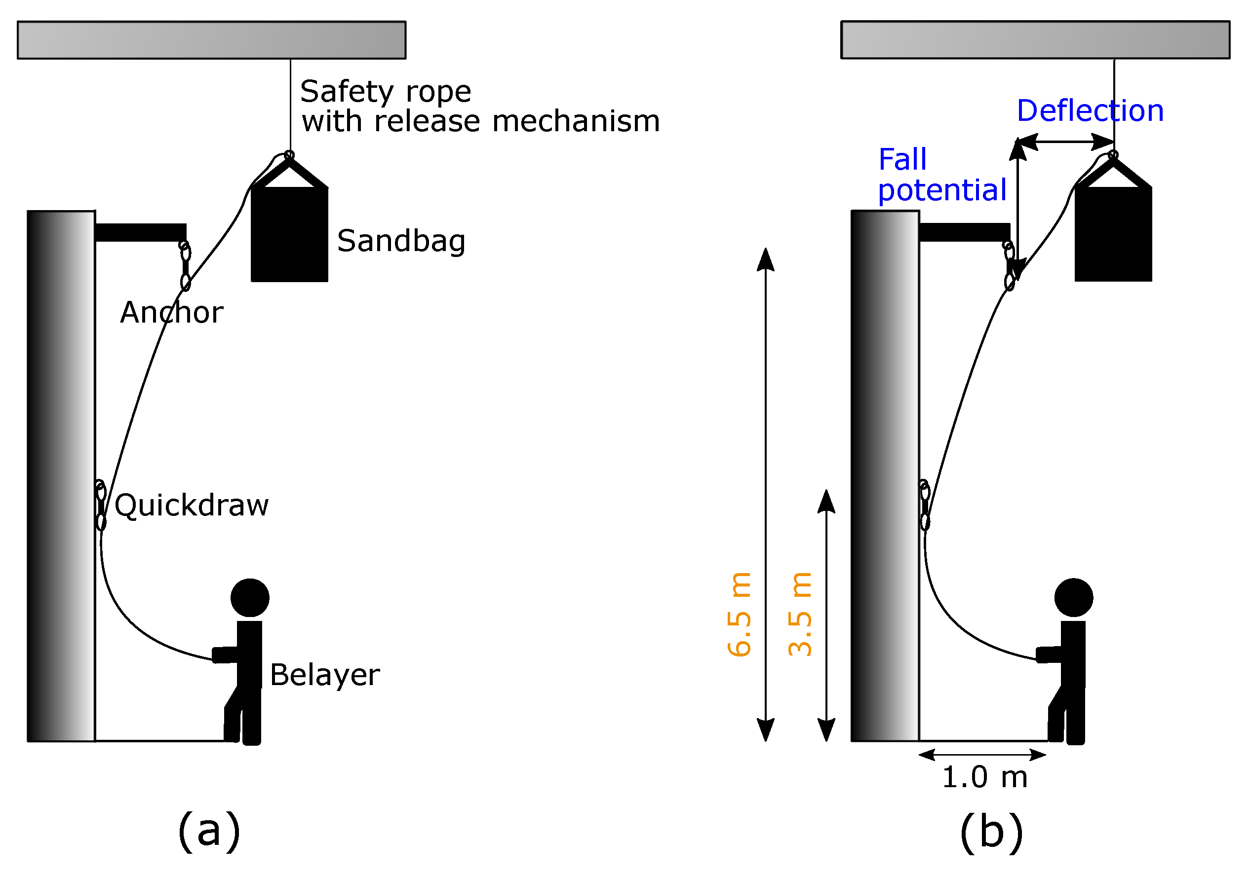
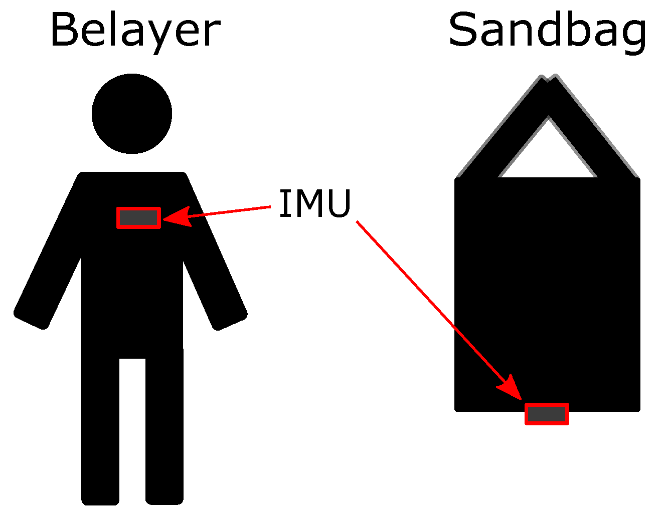
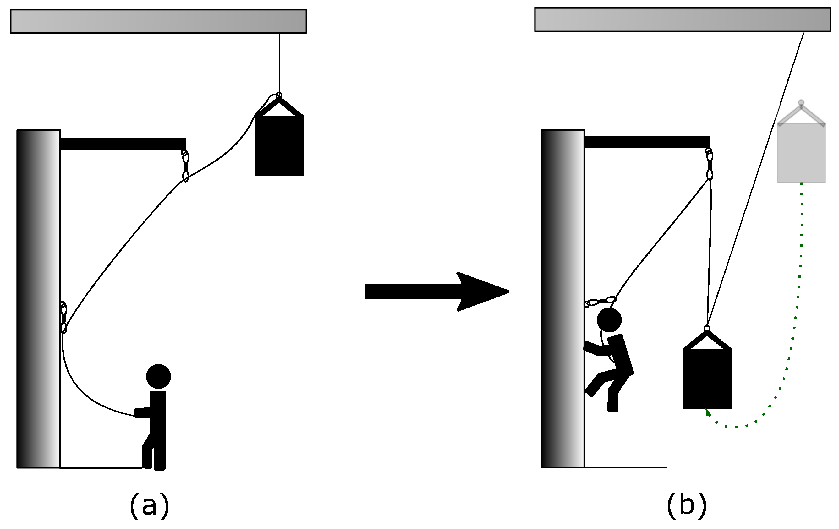
The setup as shown in Figure 1 is built around a sandbag and a belayer with identical weight of about 65 kg. Here, a sandbag served as a substitute for the climber. This guaranteed his physical integrity. In order to gather the relevant data from the falls, we were relying on three Shimmer3 IMU devices [14,15]. They allowed us to record data from both, an accelerometer and a gyroscope, in a time-synchronized way. One of the devices is positioned on the chest of the belayer and the other one onto the bottom of the sandbag, compare to Figure 2.
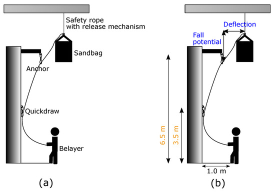
Figure 1.
(a): Overview of the experimental setup describing the scene. (b): Overview of the adjustable (blue) and fix (orange) configurations.
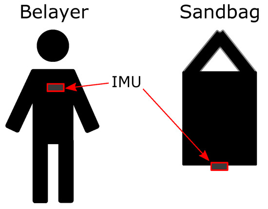
Figure 2.
Positioning of the IMU sensors on both climber and belayer.
In order to catch all the falls of the climber, the belayer operated with the belay device Eddy from the Edelrid company. It is a semi-automatic device to assist the belayer throughout climbing sequences by blocking the rope movement in a fall situation. The rope itself was running through the device, a carabiner and an anchor, to finally be connected to the sandbag. Additionally, the sandbag was fixated on the ceiling by a safety rope. This assured no unexpected ground contact. It also allowed us to re-position the sandbag for the next fall. For analyzing different fall situations, the fall potential and deflection of the climber were adjusted. Fall potential represents the vertical distance between the last clipped quickdraw and the climbers tie-in loops on his harness. In comparison, the horizontal distance is defined by the deflection. Finally, the distance of the belayer to the wall, the height of the mounted quickdraw and anchor were set to fixed values. For releasing the sandbag, a manual and mechanical mechanism was attached on top of it.
The execution of each fall can be separated in several steps. The fastest one was the fall itself, which took just two to three seconds; see Figure 3 for representative situations before and after a fall. As the climber was falling into the rope (dotted line), the belayer is beeing pulled towards the wall and carabiner. In the course of this fall situation, the belayer had two options, either belaying actively or passively. A dynamic movement behavior reducing the impact force throughout a fall is called active belaying. If, on the other side, the belayer was standing passively by, it is referenced as passive belaying. After the fall, the belayer could lower himself to the ground, the bolt of the release mechanism was locked back in and the sandbag pulled up again. Finally, the elasticity of the rope enforced a relaxation time of at least three minutes.
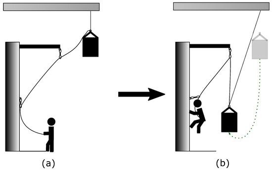
Figure 3.
Graphical representation of the events throughout a fall. (a): Initial positions of climber and belayer. (b): Situation after the fall.
2.2. Experimental Configurations
We explored several configurations to allow for a meaningful interpretation of the results. They include three different deflection and two potential fall variants. Yet, the amount of repetitions per configuration were kept at a minimum, as conducting one trial required at least seven to eight minutes of time, including the relaxation time of the rope. Each trial was conducted at least three times and repeated while belaying actively and passively. All configuration constellations are represented by Table 1. Overall, 50 trials were executed, leading to 5.12 h of recording.

Table 1.
Configurations of the trials per type of belaying.
3. Signal Processing
This section provides the pre-processing steps of the raw data from the IMUs. The sensors are able to record accelerations and angular velocities measured in a three dimensional euclidean coordinate system. Leading to three axis per sensor, namely X, Y and Z. All sensors were recording with a sampling rate of 220 Hz. For the gyroscope we used a sensitivity scale factor of per bit and a range of ±2000 /s. Respectively the accelerometer was configured with a resolution of in the range of g. For the calibration of the IMUs, we were relying on the standard procedure as defined by Shimmer [16] and Ferraris et al. [17].
3.1. Signal Extraction
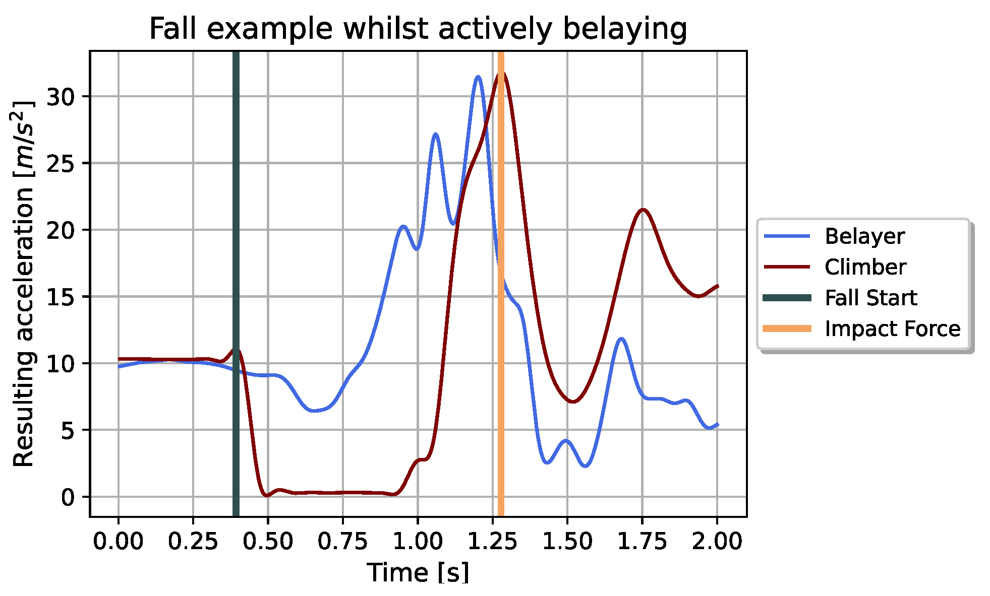
The whole recordings were stored in one file per IMU and each IMU was synchronized via Bluetooth by a master. Those single files lead to the necessity of extracting the fall sequences from the rest of the non-climb typical movements. Therefore, the free fall of the sandbag served as indication. Its resulting acceleration (Equation (1)) is dropping to almost zero throughout this situation. This behaviour can be seen in Figure 4. It visualizes the resulting accelerations recorded throughout one fall whilst actively belaying:

Figure 4.
Resulting accelerations of belayer and climber throughout a fall sequence while actively belaying. The sequences were filtered as described in Section 3.2. Additionally marked times represent starting point (grey) and endpoint (orange) of the cutted sequence. The endpoint marks the time when the impact force occurs.
We used a threshold of to identify the free falls of the climber. Afterwards, the sequences were cut to the desired length. The starting point marks the time of releasing the sandbag. It lead to a maximum slightly higher than the gravitational acceleration and could, therefore, be easily identified in the recordings. After the free fall of the climber, the resulting acceleration increases until a maximum is reached. This marks the end point of our fall sequence and is also referenced as impact force.
The belayer signals of the cutted sequences then served as input to the machine learning pipeline. As their variation within each channel was too big compared to the amount of recorded falls, we solely relied on the resulting acceleration.
3.2. Signal Filtering
In order to remove the high frequency noise in the belayer signals, a low pass butterworth filter of fourth order and a cut-off frequency of 50 Hz was applied to the accelerometer signals. The local coordinate system of the IMU was rotated into a global one relying on the Madgwick AHRS algorithm [13]. This allowed us to remove the gravitational component from the filtered signal. To remove the high frequency noise within the climber’s signal, a lowpass filter of 20th order with a cut-off frequency of 30 Hz was applied.
3.3. Signal Windowing
Windowing the sequences allowed us to further examine several areas of interest within the falls. We chose three equally dimensioned windows accounting for the time of the climbers free fall, the action of the belayer and the fall of the climber into the rope. These windows were specifically chosen to investigate their importance concerning the prediction of the impact force. We have not allowed any overlap of those windows to guarantee their separate evaluation.
4. Feature Engineering
Features were manually extracted from the pre-processed signals for each of the three windows. They can be further divided in time and frequency domain as well as coefficients from an Autoregressive model (AR) and the compressed signal of a Discrete Wavelet Transformation (DWT). Overall, we have 143 features:
- 24 features from the time domain
- 46 features from the frequency domain
- 46 features using a discrete wavelet transform
- 27 features using the coefficients from an autoregressive model.
4.1. Time Domain Features
In total, ten features belong to the time domain.
- Standard deviation absolute value of the distance between adjacent samples (DASDV), as utilized by [18]. It describes the average gradient within the sequence.where N is the amount of samples and with the value of sample i within the time series.
- The Mean absolute value (MAV), as, among others, utilized by Sarcevic et al. [19]. They applied this feature in combination with an IMU for classification.
- Sample entropy (SE) [20] as a measure for the complexity of the sequence. It is the negative of the logarithm of the relation between two template vectors A and B.The template vectors can be defined as:with being a distance measure between the sequences and . The parameter r is the maximum allowed distance and m equals the partial sequence length. In our case, we used a threshold of a fifth of the standard deviation within the window sequence for r and .
- Waveform length (WL) [21] measures the average over the absolute distance between two adjascent samples, with:To the best of our knowledge, this feature in combination with an IMU was first used by Sarcevic et al. [19] for a movement classification task.
- Root mean square (RMS) value as used by [22] as a feature for a classification task with an IMU, represents the root over the average squared value within the time series.
- Energy (E) of the windowed time signal [23].
- The hjorth parameter [24], namely activity (HA), mobility (HM) and complexity (HC), allow for a more complex representation of the time signal. The hjorth activity corresponds to the variance of the signal, whereas the mobility is a representation for a proportion of the standard deviation of the power spectrum.The complexity represents the frequency change within the signal and can be calculated as follows:
4.2. Frequency Domain Features
To each of the windowed signals, a discrete Fourier transformation was applied. Therefore, we used a hanning window of 40 and shifted the window by one. Throughout the first three frequency bands, the mean, standard deviation and maximum values were extracted as features. Additionally, three more features from the frequency domain were extracted, the spectral flux, spectral roll-off and spectral centroid. To the best of our knowledge, they were first used by Scheirer et al. [25] in the domain of speech/audio analysis.
- From the spectral flux (SF) we used the mean and standard deviation. It is a measurement on how fast the power spectrum between two adjacent windows changes and is often used in audio tasks, as Jensen et al. did in [26].whereas M is the total amount of observations and the jth observation in the frequency domain.
- The mean and the standard deviation of the spectral roll-off (SR). This feature represents the frequency at which a pre-specified percentage () of the total spectral energy lies and is often used in the audio context, as in the work by Scheirer et al. [25]. We first calculated the fraction of the total spectral energy (FTS) for each observation.with L being the total amount of frequencies within the spectrogram, the lth frequency and j the current index of the observation of the spectrogram. Finally, the spectral roll-off is given by:
- The spectral centroid (SC) describes the center of gravity of the spectrum [27]. We used the maximum center of gravity value over all observations within the given observation.with S as the norm of the spectrogram, the ith frequency and F the maximal frequency according to the Nyquist theorem.
4.3. Discrete Wavelet Transform
From the Discrete Wavelet Transform we used the detailed coefficients of the decomposed time signal as features. After looking into several wavelets, the Haar wavelet returned the most promising results. Therefore, we relied on this wavelet as the mother wavelet.
Wavelets were initially designed for the analyzation of non-stationary signals [28], and are now also utilized as features in a classification task [29].
The decomposition of the initial signal is a multi step process. Throughout each step, the signal passes a band-pass-filter and returns two coefficients, namely approximation and detailed. After each step, the time resolution of the signal is cut in half, while the frequency resolution is doubled [30]. In our case, we utilized the detailed coefficients, obtained after five steps. It results in a sufficiently short time decomposition of the signal to not fill the feature space unnecessarily whilst maintaining the characteristics of the signal. Yet, due to the differing signal lengths we received a different amount of coefficients. This was compensated by interpolating them to finally obtain 14 features per window.
4.4. Coefficients from an Autoregressive Model
Following an Autoregressive model [31]
with being the nth sample of the time signal, p the order of the autoregressive model, the ith coefficient and some white noise, we applied a conditional maximal likelihood estimator to get the coefficients [32]. As features, we used the coefficients of a model of 10th order.
4.5. The Impact Force as Label
In this study, we tried to predict the impact force. This would serve as an indicator for the severity of a climber’s fall. It is defined as the maximum force acting onto the climber during the stop of the fall by the rope. Still, higher forces can occur if the climber is hitting the surrounding wall or climbing grips. By the nature of the experimental setup, the sandbag was able to hit the wall. In the calculation of the impact force, those thereby occurring forces were neglected in the calculation.
An overview of the measured impact forces per configuration is depicted in Figure 5. The graph shows the influence of the type of belaying. Active belaying decreased the force in all situations. Yet, the greater the deflection, the less effective the proposition. Similarly, a higher fall potential lead to a higher impact force. In contrast to that, the deflection had less influence on the target value. Table 2 summarizes the average and standard deviations per configuration. Except for one case, the standard deviation increased with active belaying, while the impact force decreased. This speaks for higher movement variations within this type of belaying.
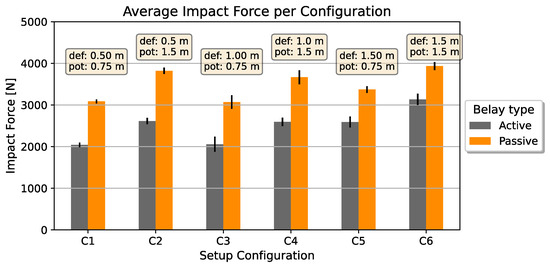
Figure 5.
Average and standard deviation of the impact force per configuration with varying deflection (def) and fall potential (pot) and the belay types.
Table 2.
Average and standard deviation of the impact force per fall configuration, further divided by the type of belaying.
5. Feature Space Reduction
The previous feature engineering process resulted in a total of 143 features. This made it necessary to investigate methods to reduce the feature space. We were able to increase the possibility of removing non-informative features and also reduced the effect of overfitting. We applied several techniques like filtering, wrapper and embedded methods as well as linear and non-linear decompositions. As the filter, wrapper and embedded methods allowed for an interpretation of the chosen feature subspace, the decomposition methods did not.
5.1. Filter Methods
Filter methods, as introduced by John and Kohavi [33], rely on the features and output variable. They choose a feature subset based on an information score between them. However, filter methods neglect the information from the regression model itself.
Two different approaches were explored. The first one is based on correlation [34] and the second one on Mutual Information (MI).
5.1.1. Pairwise Correlation
The idea behind this method is to extract a simplified uncorrelated feature subset. We calculated the correlation coefficient between all feature pairs. As most of the features did not follow a normal distribution, we used the spearman’s rank correlation coefficient [35]
with and being the standard deviations of the rank variables and their covariance. Yet, the coefficient would only allow for a suitable subspace of up to two features. To identify a higher dimensional subspace, we chose features based on the average correlation information between all features. Then, we selected the ones with the least overall correlation.
5.1.2. Mutual Information
Mutual Information can be used as a measure for the amount of information obtained for one variable while knowing a value of another variable. It uses entropy as a measurement. We applied the Mutual Information in combination with the nearest neighbor approach, as proposed by [36]. There, the Shannon’s entropies are estimated based on the average distance to the k nearest neighbors. The amount of allowed neighbors was set to three.
5.2. Wrapper Methods
Filter methods choose a feature subset based on a score value between feature pairs. In contrast to that, wrapper methods utilize machine learning algorithms for the selection process. We used Recursive Feature Elimination (RFE) as a selection algorithm, as described by Guyon et al. [37]. It is an iterative approach removing the least two important features after each iteration. A linear Support Vector Regressor (SVR) was used to identify the importance by assigning weights to the features [38]. The iteration process was proceeded until the desired number of features is left.
5.3. Embedded Methods
Embedded methods choose the feature subspace throughout the training process of the machine learning algorithm [39]. Two of those methods were evaluated within this paper. The first one uses an -regularizer [40,41] and the second one is based on decision trees [42].
5.3.1. -Regularizer
, also known as Lasso regularization [43], applies a penalty term onto the cost function of a linear model. The objective is to minimize
whereas is the penalty term with and the feature vector. As the penalty term will increase with the amount of features, this method will cause sparsity through the norm, hence serving as feature selection algorithm [44].
5.3.2. Random Forest
A Random Forest is an ensemble of multiple decision trees. Each tree within the forest randomly chooses a subset of features. A split within a tree is based on a single feature. This serves as an indicator for the feature importance. Within a regression, the split is done, based on the mean squared error. We set the number of required samples for a split equal to two and the maximum depth up to 10 splits. Those settings were then applied to 1000 decision trees.
Correlated features hold a similar importance, making decision trees vulnerable to keeping the variance low. Therefore, we applied a pre-filtering step in order to sort out highly correlated features. This was done by using hierarchical clustering with a distance of five on the pairwise correlation matrix. The method is similar to the one used by Chavent et al. [45]. For easier interpretation of the results, we selected one of the features instead of choosing the centroid from clustering.
5.4. Decomposition Methods
The intention of decomposition methods is to reduce the feature dimension space while retaining essential information within the data set. It can be differentiated between linear and non-linear decomposition methods. For the linear approach, we used the Principle Component Analysis (PCA) [46,47]. To achieve the non-linearity, the PCA was adapted by applying the kernel trick to it [48]. We used a gaussian radial basis function as kernel.
5.5. Comparison Method
A random feature selection model served as a baseline reference in order to evaluate the feature reduction methods. It also served as an indication towards the plausibility of the prediction model itself. The random selection process begins with a random permutation of the feature columns. Then, the first k with features are chosen. Additionally, the complete feature space served as a second baseline.
6. Predictors
This section provides an overview of the applied predictors and their configuration setup. Two were utilized, a Support Vector and a Random Forest Regressor. Both are supervised learning algorithms, hence requiring a label for training. Additionally, the trials were split in a k-fold cross validation like manner with , to obtain a prediction for each trial individually. This allowed us to have 49 samples for training and one for testing within every cross-validation step.
In order to identify suitable hyperparameter, we performed a tenfold cross-validated grid search within each of the 50-fold cross-validation steps. The separation of the samples was accomplished by the GridSearchCV method from the scikit-learn package.
6.1. Support Vector Regressor
SVR tries to identify a hyperplane that fits most of the samples while also reducing the margin violations, expressed by an -tube [49]. The parameter was set to . Additionally, we used a gaussian radial basis function as kernel to make the decision function non-linear. The regularization hyperparameter C was set to be either 1, 5 or 10, based on the grid search result.
6.2. Random Forest Regressor
A Random Forest Regressor on the other hand is an ensemble of multiple decision trees. Each tree is performing a prediction based on a different assumption. The results are then averaged and returned as the prediction. In the training process, the algorithm is splitting the hyperspace into regions and averages the target values within them. Those regions are fit in order to perform predictions close to the true value. This process can easily lead to overfitting if no restrictions are applied. Therefore, a maximum depth for each tree of 5, 10 or 20 was allowed and at least two samples were required in order for a node to split. As split criterion, the mean squared error was applied. Within the grid search, we set the amount of trees to 250, 500 and 1000. With the SVR, we assumed the data achieves best results by kernelizing it with a radial basis function. Such an assumption was not necessary with a decision tree. It is able to adapt itself to the data.
6.3. Error Metric
One of the main challenges with the 50 recorded trials were multiple setup configurations and a scant amount of repetitions. This lead to a high variation in the prediction error. Therefore, we chose the first, second and third quartiles as a metric to evaluate and compare the prediction results. They were calculated for each sample in the test sets throughout the cross-validation process.
6.4. Software Specification
In order to generate the results, we used the script language Python version 3.8.3 in combination with the in scikit-learn version 1.0.1 implemented regressor and feature dimension reduction methods. If not otherwise specified, the default hyperparameter were used.
7. Results
This chapter describes the obtained results. It starts with the overall results for each feature reduction method. Then, we will go deeper into the interpretation by analyzing the chosen feature subspace with respect to the prediction results. Finally, we chose one specific trial for further analysis and to get a better understanding of the underlying results.
7.1. Impact of the Type of Belaying
According to the results of a statistical t-test, active belaying reduces the impact force significantly compared to passive belaying. In combination with a Shapiro-Wilk test, which showed that both classes follow a Gaussian distribution, the evidence speaks against the null hypothesis whilst using a threshold of .
7.2. Predictor Results
For simplicity, in the further analyzations we talk about metric errors in percent. As an example, the values from Table 2 will be used. In total, the average measured impact force while actively belaying was 2505.52 N with an averaged standard deviation of 101.98 N. Table 3 summarizes the least prediction errors for each applied dimension reduction technique, including the ones from the basline model. There, the smallest median error is listed at about 4.96% and, hence, would result in a total median error of about 124.27 N. This is higher than the averaged standard deviation, though, smaller than the highest standard deviation in one specific configuration (fall potential of one meter and a deflection of 0.75 m).
Table 3.
Regressor performances as metric error with or without feature reduction methods utilizing features from all windows with the resulting acceleration as input signal. The percentages represent the error towards the true value based on the associated quartiles. Green colored values depict the best results per column and red the worst.
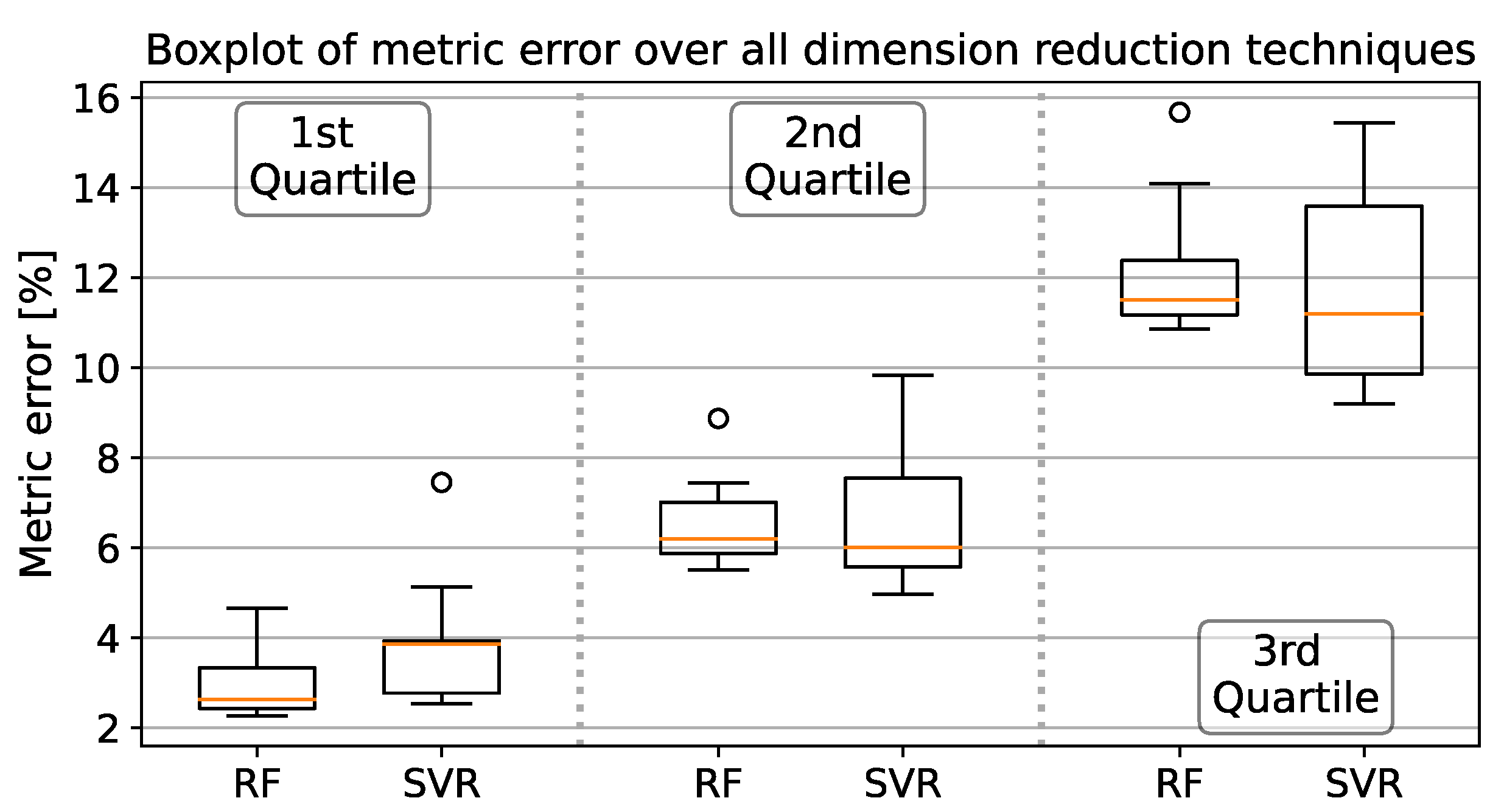
As listed in Table 3, the SVR in combination with the two decomposition methods returned valid results with a median error of (PCA) and (kernel PCA). However, they both were outperformed by the second baseline model in the third quartile error.
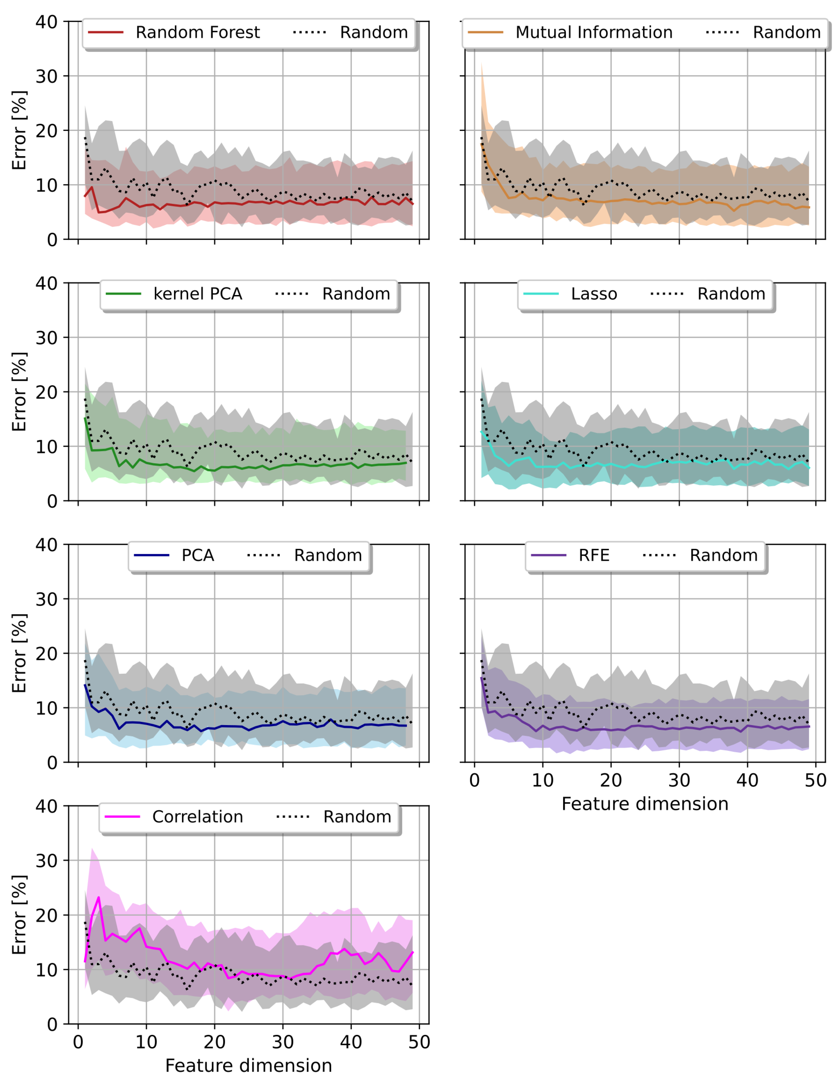
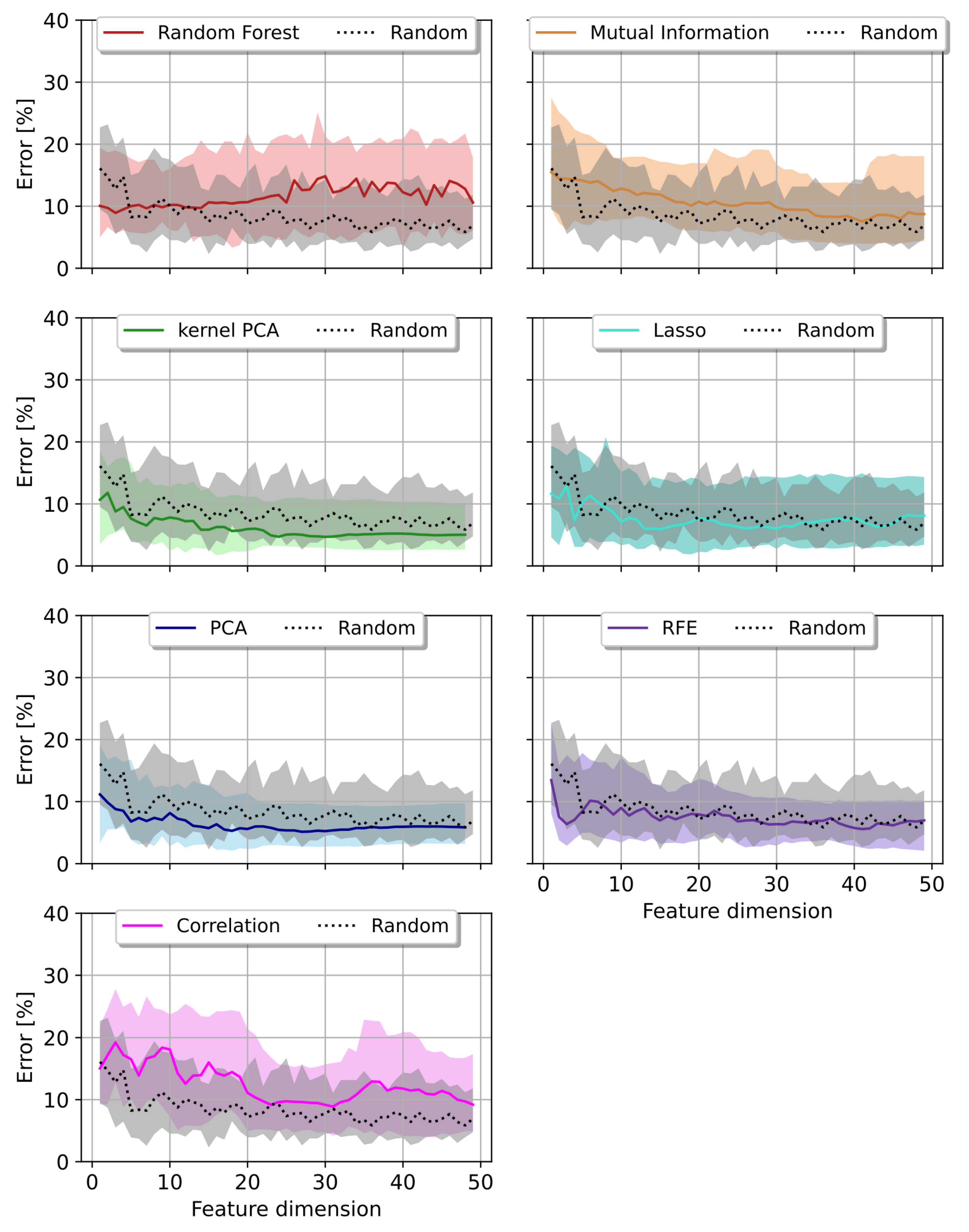
Figure 6 visualizes the three quartile errors throughout the course of the first 49 feature dimensions, obtained by utilizing the SVR for the prediction task. There, they are compared to the random baseline model. PCA and kernel PCA were the only two models staying below this baseline in the second and third quartile error.
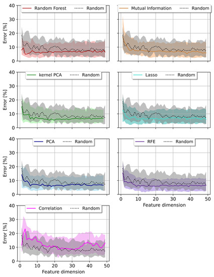
Figure 6.
Prediction error per feature dimension reduction method (colored curves) compared to a Random feature selection algorithm (black/grey) using Random Forest as regressor. The median error with first and third quartiles are shown.
We achieved lower metric error results with Random Forest and the correlation method. Their quartile errors were above the random baseline for most of the surveyed feature dimensions.
Figure 7 summarizes the results from Table 3 in a boxplot. Within each quartile error, SVR results had a wider error range than with the Random Forest regressor.
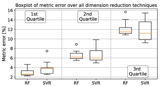
Figure 7.
Summarized metric errors from Table 3 separated by Regressors and quantile errors.
The outcomes from the RF varied from the SVR as Lasso and Random Forest outperformed the decomposition methods. Lasso achieved best results in the first and Random Forest in the second quartile error. Both methods stayed below the baseline errors in a low dimensional feature space of less than 15 features, cp. Figure 8. Random forest for feature selection utilized an identical predictor as the regressor itself, hence the good results. Though, no signifcant performance improvement towards the other methods could be observed. PCA and kernel PCA did also produce viable results below the two baseline models in the first and second quartile errors. The non-linearity of the kernel PCA even outperformed the first mentioned in all error metrics.

Figure 8.
Prediction error per feature dimension reduction method (colored curves) compared to a Random feature selection algorithm (black/grey) using a Support Vector Machine as regressor. The median error with first and third quartiles are shown.
7.3. The Chosen Feature Subspace
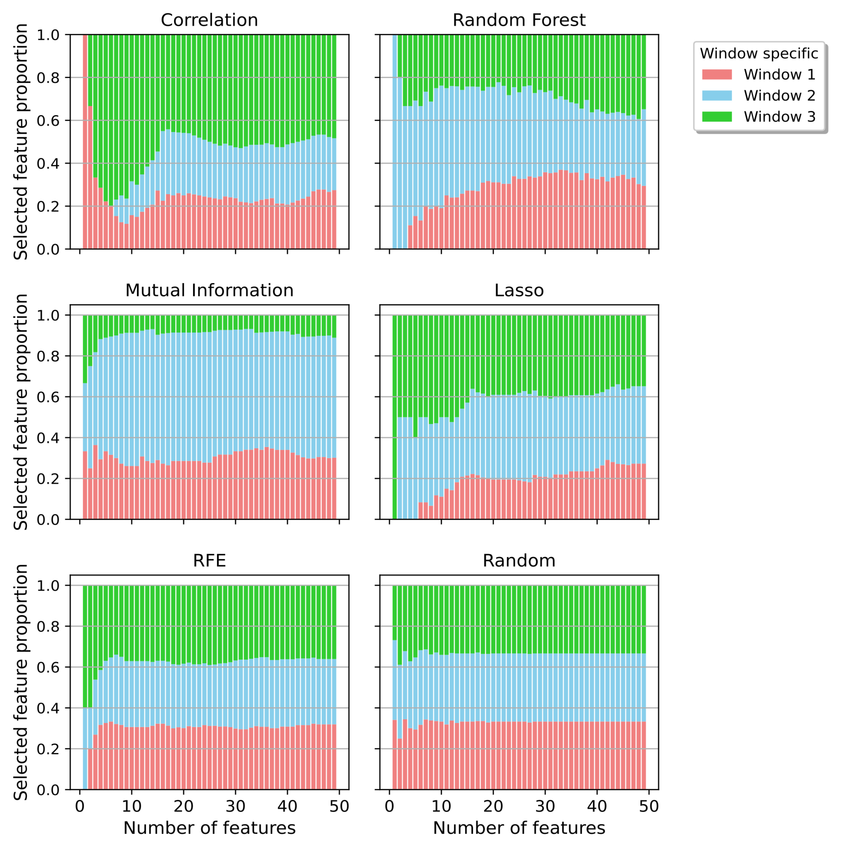
Figure 9 categorizes for each feature subspace the amount of chosen features from each window. Figure 10 visualizes a finer categorization by separating the windows further into their respective feature domains. Interestingly, all methods selected at least of the features from Window 1.
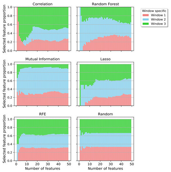
Figure 9.
Proportion of all features categorized by the pre-chosen windows and separated by the feature reduction techniques.
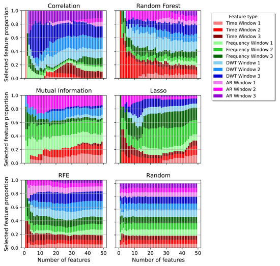
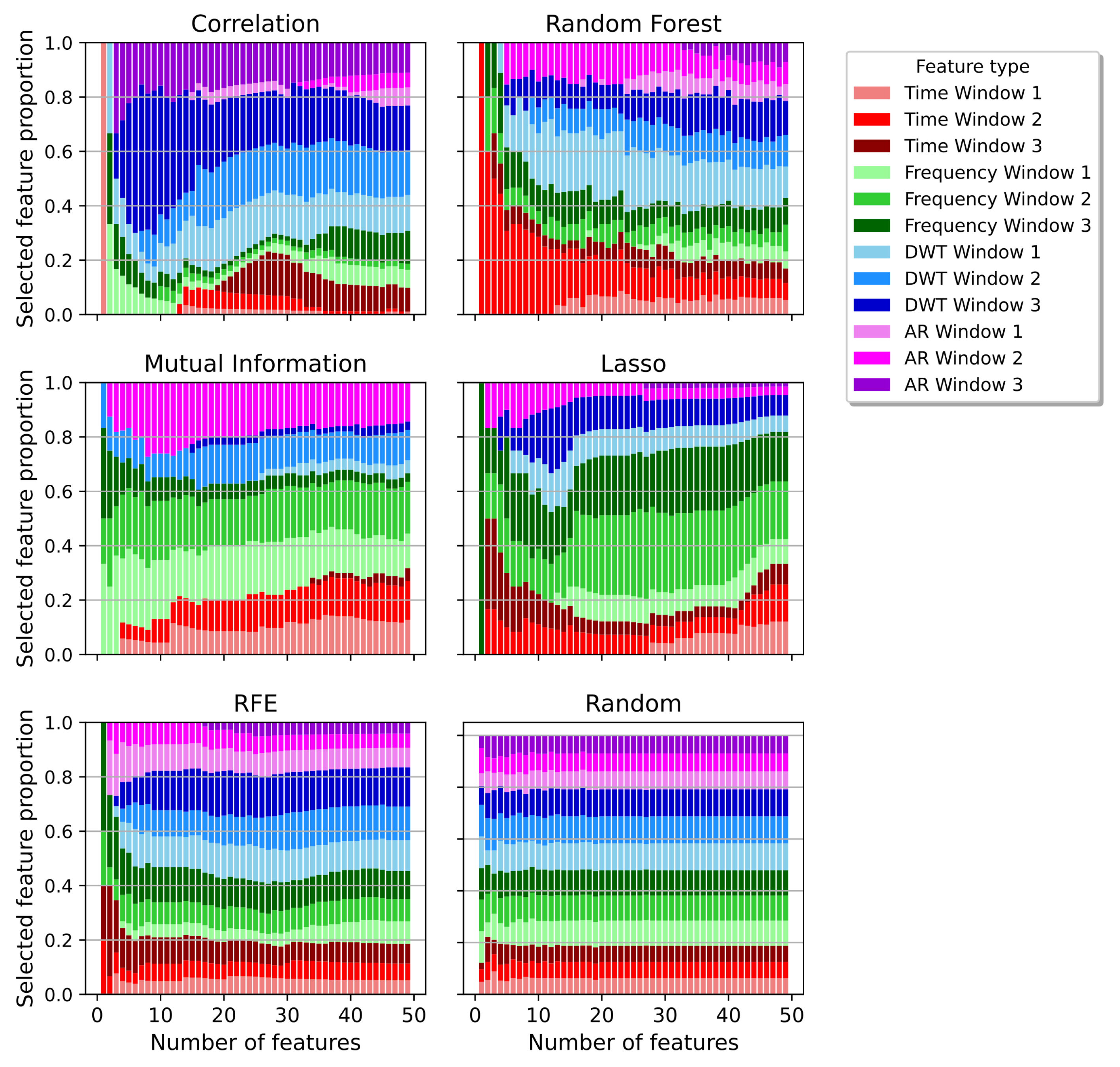
Figure 10.
Proportion of all features categorized by the pre-chosen windows and the feature types.
The correlation method selected most features from Window 3. Those mainly did belong to the DWT and AR type of features, both, partially describing the input signal. Yet, the correlation method performed worse compared to all other applied methods.
Mutual Information was the second of the two applied filter methods. It performed better than the correlation, but was still worse than most of the other ones. The method chose the least features from Window 3. Most of them did belong to the frequency domain, which was also selected the most overall.
Both embedded methods, Lasso and RF, showed differences in their choice of a suitable subspace. For lower dimensions, Lasso selected a high proportion of about 50% from Window 3. For higher dimensions, the proportion declined. This behaviour was the opposite with the Random Forest method. Both methods also differed in their choice of feature types. Lasso favored the frequency domain, whereas Random Forest preferred features from the DWT. Features from the frequency domain accounted for the smallest part.
The feature types of the Lasso method changed significantly between a feature subspace of 14 and 16 features. This was also perceptible in the prediction errors, especially with the RF regressor.
The wrapper method was the only one balancing the types of features in a low and high dimensional space. The same accounted for its choice of window type. It showed a homogenous profile. Interestingly, this stability could also be seen in the quartile errors over the feature spaces with an RF as regressor. Based on the prediction errors, this method had a valid performance with a median error of 5.87%.
Table 4 references the three highest ranked features chosen by the corresponding feature selection algorithms. The proportion column represents how often the specific feature was chosen by the algorithm. Except for RFE, this value is comparable between all methods. All methods chose features from several categorical types. However, the ones from the frequency domain dominated, whereas one of the most re-occuring features was the maximum of the spectral centroid. The Hjorth parameter and the wave length were mainly selected from the time domain. Wave length performed best as a single feature with a first quartile error of , a median of and a third quartile error of .
Table 4.
Prediction errors of most chosen features per selection method. The bottom part of the table displays the prediction errors while all features from the corresponding windows are used. Green colored values depict the best results per column and red the worst.
The correlation method was the only method that selected features from Window 1. They were also the ones with the worst performance individually.
The bottom three columns of Table 4 reveal the prediction errors when all features from the corresponding window were used for prediction. While Window 1 features returned the highest errors with an RF regressor, they did beat Window 3 if a Support Vector Machine was utilized as regressor. Nonetheless, each window individually performed worse than the baseline model using the whole feature space.
7.4. Trial Individual Analyzation
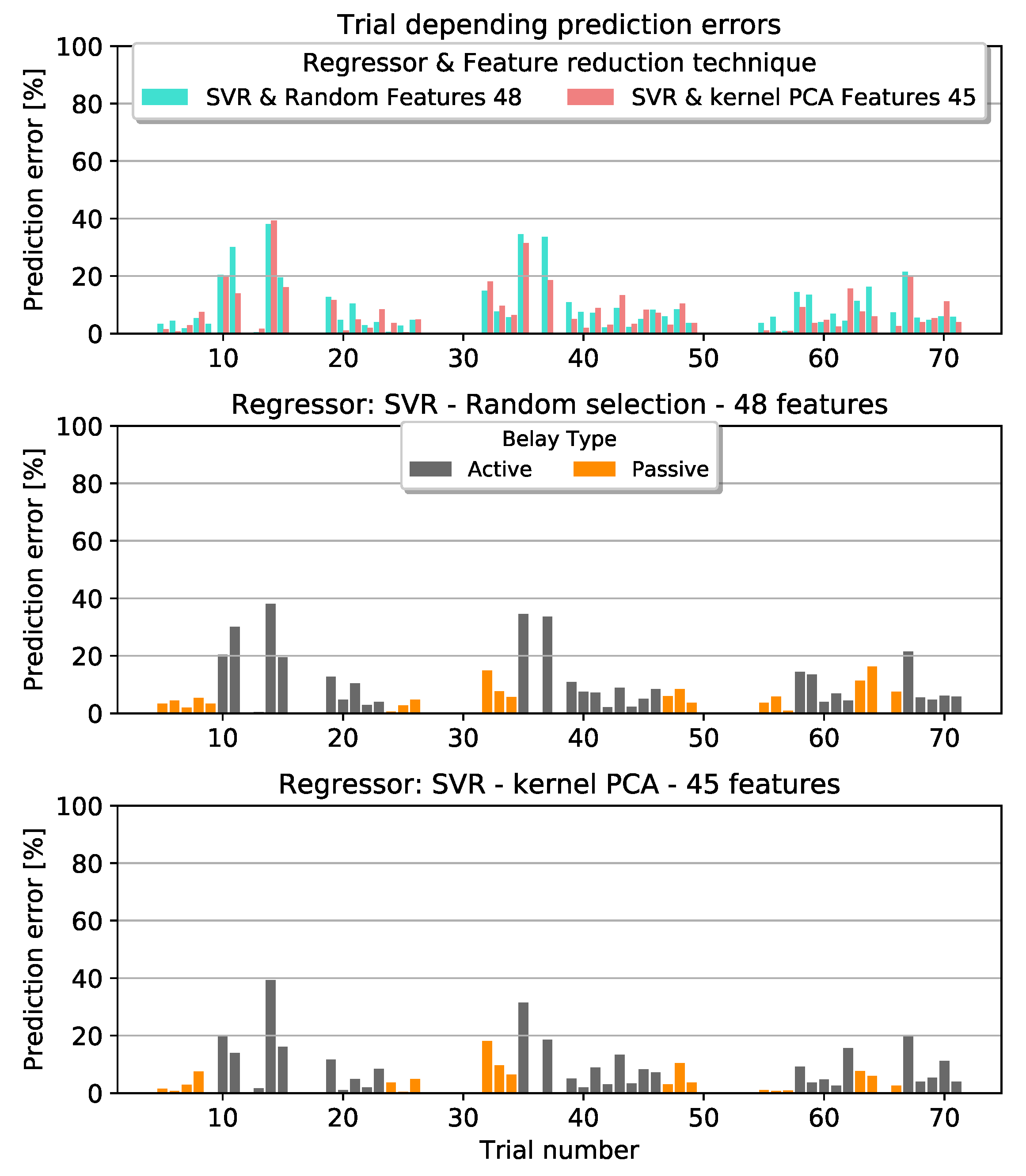
This section provides a deeper analyzation of the prediction errors. Kernel PCA in combination with an SVR and a feature subspace of 45 dimensions was able to drop the median error to less than 5% and outperformed all other methods. Figure 11 visualizes the specific trials. They are compared to the random feature selection method. Both methods revealed difficulties in the prediction of analogous trials. Some of them differed from the true value by over . Splitting the trials into their type of belaying revealed that active belaying was responsible for the prediction errors. Additionally, we tested the kernel PCA method with 45 features against the full feature space for any significant improvements. According to a statistical t-test, there exist no evidence for it. It was tested with an alpha level of .
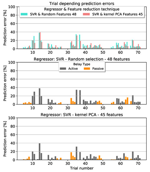
Figure 11.
Trial depending prediction errors with a Support Vector Machine as Regressor. Top graph: Comparison between the two feature dimension reduction techniques kernel PCA and Random. Middle and Bottom graph: Visualization of the prediction error separated into active and passive type of belaying based on the results from the Random and kernel PCA method respectively.
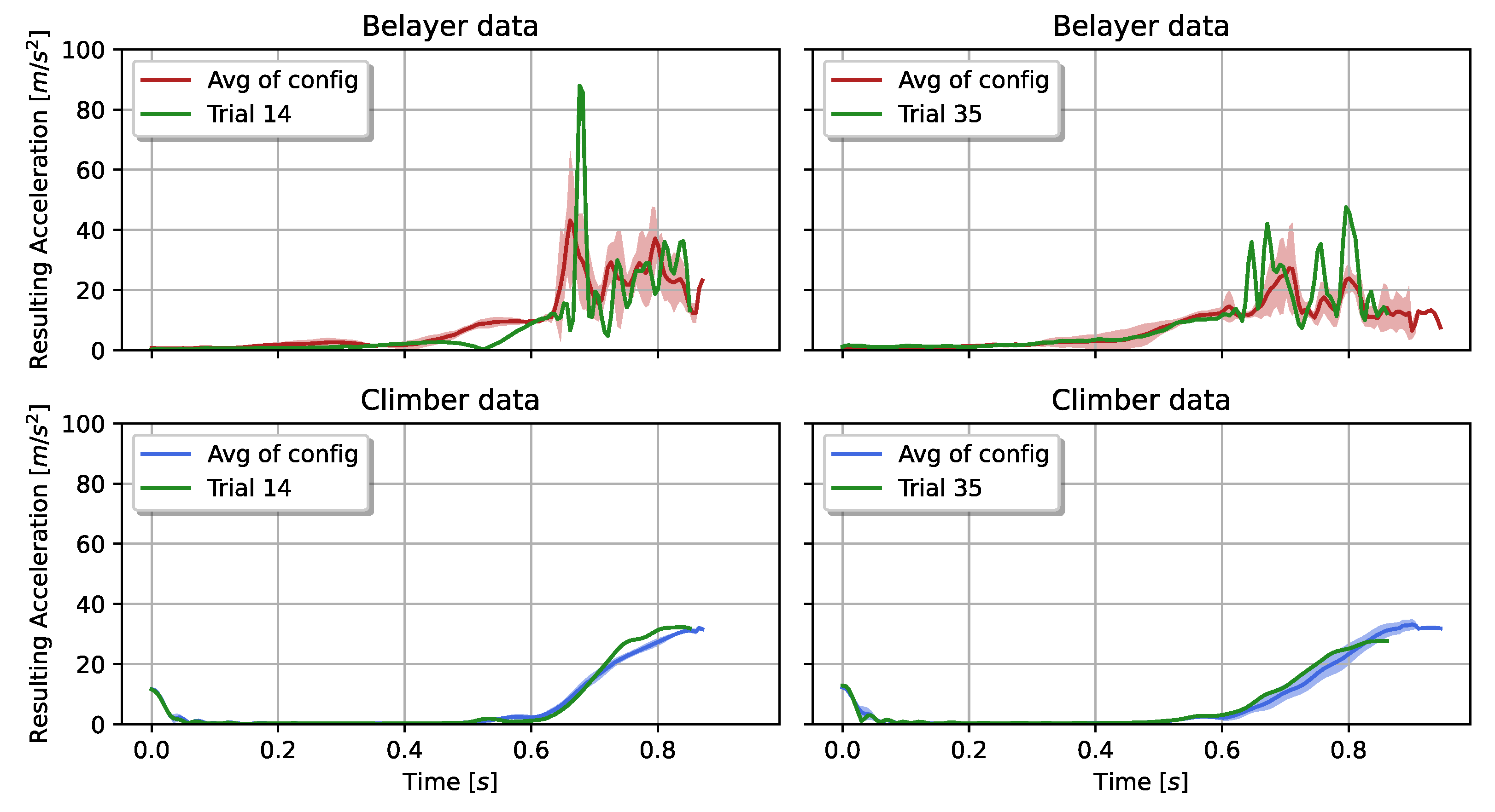
Two exemplary input signals from climber and belayer are visualized in Figure 12. Both trials belong to the category of active belaying with a fall potential of m and a deflection of m (left) and 1 m (right). Each displayed trial reflects a certain difficulty. The first example describes a varying input signal (left graph). Its maximum resulting acceleration exceeded the 80 and was, hence, twice as much as the average maximum from the rest of the recorded trials with the same configuration. Yet, their impact forces varied only slightly with in the specific trial. In comparison, the average impact force from all other trials was about () N.
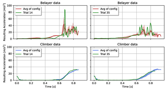
Figure 12.
Resulting accelerations from climber and belayer of the trials with highest prediction errors. Green: individual trial example; mean and standard deviation of the climber signal (blue) and the belayer signal (red) from the same fall configuration as the trial example.
The second example (right graphs), shows comparable curve progressions with a lower response in the impact force. It recorded higher accelerations of almost times as much as the average. Yet, the impact force dropped from N to N.
8. Discussion
This paper shows a potential in the prediction of climb-specific events, based on sensors worn by the belayer. Our setup was built to record pendulum falls in sports climbing with different variations of fall parameters for climber and belayer, with the aim to estimate the resulting impact force. The belayer was switching between actively and passively belaying.
8.1. Variation in the Sample Space
In Figure 11 we can see that highest prediction errors were achieved while active belaying was taking place. One explanation is that in this situation the belayer is standing still before being pulled towards the wall, leading to a small space of variations. With active belaying the movement pattern starts to vary. The top left graph in Figure 12 shows an example for this behavior. In trial 14 the belayer initiated the active reaction as a “jump” later than within the rest of the trials’ same configuration. This had an effect on the recorded impact force of the climber. Generally, the impact force varied more whilst actively belaying, compared to Table 2. Therefore, the amount of repetitions per configuration in combination with the highly varying movement patterns of the belayer are challenges to overcome in the future.
8.2. Interpretable Methods
We divided the input signals per trial in three non-overlapping windows. This allowed us to distinguish between the three different movement behaviors of the belayer. In Window 1, the climber was experiencing a free fall, whilst the belayer was performing non-belay typical movements. Interestingly, all of the interpretable feature reduction techniques chose a significant amount of features from this specific window. The explanation might lie in the high variations within Window 3. There, the climber was falling into the rope, hence, pulling the belayer towards the wall. It is also the window where the impact force is taking place. Depending on the countermeasure taken by the belayer against the fall, the timing of the “jump” varied within every trial. The results from the Mutual Information and Correlation methods from Window 3 underline this finding. The first approach measured the dependencies between the features and their corresponding label. This means that there was almost no information gain towards the impact force by relying on Window 3 features. On the other side, the correlation method chose the highest amount of features from Window 3. This approach built its feature map based on dissimilarities within each feature, leading to the fact, that we had the highest variation between features from this window. Going a bit deeper into details, we could identify the DWT and AR features being responsible for the high variation within features from Window 3. DWT decomposes the signal into a set of wavelets, whereas AR stores the information in the form of a linear combination. As the recorded signals were mostly unique in-between all trials, this was leading to unique feature profiles within the two categories.
Window 2 contained the highest information gain for differentiating between active and passive belaying, which is also an indication towards the impact force, as shown in Figure 5. Therefore, it is not surprising for the selection algorithms to choose from there. Interestingly, the three highest ranked features from the interpretable methods, except for correlation, were chosen from Window 2 or 3.
8.3. Decomposition Methods
As well as the decomposition methods worked in combination with the SVR, it is more difficult to interpret the results. We are not able to draw a conclusion towards the individual features themselves. However, it allows us to analyze the feature subspace. The subspace seems to be well spread in order to handle the task of predicting the impact force, as the best median error resulted in a deviation of less than .
9. Conclusions and Outlook
Utilizing the estimation of the impact force throughout a fall in a training environment could improve the quality of a belayer. We could identify the influence of the type of belaying regarding the impact force, cp. Figure 5. By belaying actively, we were able to reduce it by up to . And reducing it should always be one of the priorities as a belayer. A device worn by the climber would be able to monitor this parameter. However, we wouldn’t be able to clearly identify the belayer as the cause. Therefore, we focused on a monitoring system attached to the belayer.
We developed a machine learning model to handle the prediction of the impact force based on the movement behaviour of the belayer throughout pendulum falls. The best results were achieved with a median error of . However, outlier errors mark a difficulty within the data set. Further analyzations of those outliers revealed a high varying input signal and/or label as the cause. This lead to the conclusion of sparse repetitions per configuration.
In our study, we could show the importance of the pre-defined windows and the feature reduction techniques. Those techniques failed to improve the prediction of the impact force significantly; however, they serve as an indication for interpreting the results regarding their plausibility.
Depending on the type of belaying, each window represents an independent signature. Window 3 directly covers the climbers’ fall into the rope. Neglecting the Mutual Information method, the other methods showed a high relevance towards this window. However, each selection method chose features from all windows.
Independent from the selection method, the most re-occuring features did belong to the frequency domain and either Window 1 or 2. This underlines the plausibility of the chosen subspaces.
We showed that the correlation method is a suitable indicator for the individuality of the sequences within each window. Most of them did belong to Window 3, where the belayer got pulled towards the wall. A high proportion of those features could be assigned to the DWT or Autoregressive coefficients.
Limitations in the sample space as well as high variability in the belayer’s movements are challenges to overcome in the future. Still, our results have the capability to serve as a support and feedback system for climbing. Further developments involve the analyzation of different climb specific activities.
Future work has to be done by collecting more data in order to improve the performance. This includes different types of configurations, like falls from a straight or even positive wall, as well as falls with real climbers.
Within this paper, we saw a glimpse of what might be possible in a sensor worn system by a belayer. It would be interesting to see its limitations. Sports climbing in particular could benefit from such a system, as it wouldn’t interact with the climber itself. It could be utilized in a training environment to support and improve the skills of a belayer. However, improvements need to be done in order to guarantee stable results with reduced prediction errors.
Manual feature engineering is also a difficult task, as one is never guaranteed to choose the optimal features for the task. Therefore, with a larger dataset, other features, feature-types or deep learning approaches with automatic feature engineering might improve the results even further.
Author Contributions
Conceptualization, M.M.; Data curation, H.O.; Formal analysis, H.O. and M.M.; Funding acquisition, M.M.; Investigation, H.O. and M.M.; Methodology, H.O. and M.M.; Project administration, M.M.; Resources, M.M.; Software, H.O. and M.M.; Supervision, M.M.; Validation, H.O. and M.M.; Visualization, H.O.; Writing—original draft, H.O.; Writing—review & editing, M.M. All authors have read and agreed to the published version of the manuscript.
Funding
This project was funded by the Federal Ministry for Economic Affairs and Energy (BMWi) and their Central Innovation Programme (ZIM) for small and medium-sized enterprises (SMEs).
Institutional Review Board Statement
Not applicable.
Informed Consent Statement
Not applicable.
Data Availability Statement
No open data availability.
Acknowledgments
We acknowledge the safety research department of the German Alpine Club and the Edelrid GmbH & Co. KG for their support and contribution throughout this research project.
Conflicts of Interest
The authors declare no conflict of interest.
References
- Neuhof, A.; Hennig, F.F.; Schöffl, I.; Schöffl, V. Injury risk evaluation in sport climbing. Int. J. Sports Med. 2011, 32, 794–800. [Google Scholar] [CrossRef] [PubMed]
- Schöffl, V.; Morrison, A.; Schwarz, U.; Schöffl, I.; Küpper, T. Evaluation of injury and fatality risk in rock and ice climbing. Sports Med. 2010, 40, 657–679. [Google Scholar] [CrossRef] [PubMed]
- Schöffl, V.R.; Hoffmann, G.; Küpper, T. Acute injury risk and severity in indoor climbing-a prospective analysis of 515,337 indoor climbing wall visits in 5 years. Wilderness Environ. Med. 2013, 24, 187–194. [Google Scholar] [CrossRef] [Green Version]
- Sascha, W. Kletterhallen-Unfallstatistik 2019. Available online: https://www.alpenverein.de/bergsport/sicherheit/unfallstatistik/kletterhallen-unfallstatistik-2019_aid_35738.html (accessed on 24 November 2021).
- Ivanova, I.; Andrić, M.; Moaveninejad, S.; Janes, A.; Ricci, F. Video and Sensor-Based Rope Pulling Detection in Sport Climbing. In MMSports ’20: Proceedings of the 3rd International Workshop on Multimedia Content Analysis in Sports; Association for Computing Machinery: New York, NY, USA, 2020; pp. 53–60. [Google Scholar] [CrossRef]
- Kim, J.; Chung, D.; Ko, I. A climbing motion recognition method using anatomical information for screen climbing games. Hum.-Centric Comput. Inf. Sci. 2017, 7, 25. [Google Scholar] [CrossRef] [Green Version]
- Ladha, C.; Hammerla, N.Y.; Olivier, P.; Plötz, T. ClimbAX. UbiComp 2013. In Proceedings of the 2013 ACM International Joint Conference on Pervasive and Ubiquitous Computing, Zurich, Switzerland, 8 September 2013; pp. 235–244. [Google Scholar] [CrossRef]
- Kosmalla, F.; Daiber, F.; Krüger, A. ClimbSense: Automatic Climbing Route Recognition Using Wrist-Worn Inertia Measurement Units. In Association for Computing Machinery; Association for Computing Machinery: New York, NY, USA, 2015; pp. 2033–2042. [Google Scholar] [CrossRef]
- Boulanger, J.; Seifert, L.; Herault, R.; Coeurjolly, J.F. Automatic Sensor-Based Detection and Classification of Climbing Activities. IEEE Sens. J. 2016, 16, 742–749. [Google Scholar] [CrossRef]
- Pansiot, J.; King, R.C.; McIlwraith, D.G.; Lo, B.P.L.; Yang, G. ClimBSN: Climber performance monitoring with BSN. In Proceedings of the 5th International Summer School and Symposium on Medical Devices and Biosensors, Hong Kong, China, 1–3 June 2008. [Google Scholar] [CrossRef]
- Bonfitto, A.; Tonoli, A.; Feraco, S.; Zenerino, E.C.; Galluzzi, R. Pattern recognition neural classifier for fall detection in rock climbing. Proc. Inst. Mech. Eng. Part P J. Sport. Eng. Technol. 2019, 233, 478–488. [Google Scholar] [CrossRef]
- Tonoli, A.; Galluzzi, R.; Zenerino, E.C.; Boero, D. Fall identification in rock climbing using wearable device. Proc. Inst. Mech. Eng. Part P J. Sport. Eng. Technol. 2016, 230, 171–179. [Google Scholar] [CrossRef]
- Munz, M.; Engleder, T. Intelligent Assistant System for the Automatic Assessment of Fall Processes in Sports Climbing for Injury Prevention based on Inertial Sensor Data. Curr. Dir. Biomed. Eng. 2019, 5, 183–186. [Google Scholar] [CrossRef]
- ShimmerSensing. Shimmer: User Manual Revision 3p. 2017. Available online: https://shimmersensing.com/wp-content/docs/support/documentation/Shimmer_User_Manual_rev3p.pdf (accessed on 24 November 2021).
- ShimmerSensing. Shimmer3: Spec Sheet v.1.8. 2019. Available online: https://shimmersensing.com/wp-content/docs/support/documentation/Shimmer3_Spec_Sheet_V1.8.pdf (accessed on 24 November 2021).
- ShimmerSensing. 9DoF Calibration Application: User Manual Rev 2.10a. 2017. Available online: https://shimmersensing.com/wp-content/docs/support/documentation/Shimmer_9DOF_Calibration_User_Manual_rev2.10a.pdf (accessed on 24 November 2021).
- Ferraris, F.; Grimaldi, U.; Parvis, M. Procedure for effortless in-field calibration of three-axis rate gyros and accelerometers. Sens. Mater. 1995, 7, 311–330. [Google Scholar]
- Yu, S.; Jeong, E.; Hong, K.; Lee, S. Classification of nine directions using the maximum likelihood estimation based on electromyogram of both forearms. Biomed. Eng. Lett. 2012, 2, 129–137. [Google Scholar] [CrossRef]
- Sarcevic, P.; Kincses, Z.; Pletl, S. Wireless Sensor Network based movement classification using wrist-mounted 9DOF sensor boards. In Proceedings of the 2014 IEEE 15th International Symposium on Computational Intelligence and Informatics (CINTI), Budapest, Hungary, 19–21 November 2014; pp. 85–90. [Google Scholar] [CrossRef]
- Richman, J.S.; Moorman, J.R. Physiological time-series analysis using approximate entropy and sample entropy. Am. J. Physiol. Heart Circ. Physiol. 2000, 278, H2039–H2049. [Google Scholar] [CrossRef] [Green Version]
- Lotte, F. A new feature and associated optimal spatial filter for EEG signal classification: Waveform Length. In Proceedings of the 21st International Conference on Pattern Recognition (ICPR2012), Tsukuba, Japan, 11–15 November 2012; pp. 1302–1305. [Google Scholar]
- Zhang, M.; Sawchuk Alexander, A. A Bag-of-Features-Based Framework for Human Activity Representation and Recognition. In Proceedings of the 2011 International Workshop on Situation Activity & Goal Awareness (SAGAware ’11), Beijing, China, 18 September 2011. [Google Scholar] [CrossRef]
- Rihaczek, A. Signal energy distribution in time and frequency. IEEE Trans. Inf. Theory 1968, 14, 369–374. [Google Scholar] [CrossRef]
- Hjorth, B. EEG analysis based on time domain properties. Electroencephalogr. Clin. Neurophysiol. 1970, 29, 306–310. [Google Scholar] [CrossRef]
- Scheirer, E.; Slaney, M. Construction and evaluation of a robust multifeature speech/music discriminator. In Proceedings of the 1997 IEEE International Conference on Acoustics, Speech, and Signal Processing, Munich, Germany, 21–24 April 1997; pp. 1331–1334. [Google Scholar] [CrossRef]
- Jensen, K.; Andersen, T.H. Real-Time Beat EstimationUsing Feature Extraction. In Computer Music Modeling and Retrieval; Wiil, U.K., Ed.; Springer: Berlin/Heidelberg, Germany, 2004; pp. 13–22. [Google Scholar]
- George, T.; Georg, E.; Perry, C. Automatic musical genre classification of audio signals. In Proceedings of the 2nd International Symposium on Music Information Retrieval, Indiana University, Bloomington, IN, USA, 15–17 October 2001. [Google Scholar]
- Polikar, R. The story of wavelets. In Physics and Modern Topics in Mechanical and Electrical Engineering-World Scientific and Engineering Academy and Society; Phys. Mod. Topics Mech. Electr. Eng.; Iowa State University: Ames, IA, USA, 1999; pp. 192–197. [Google Scholar]
- Zhu, C.; Yang, X. Study of remote sensing image texture analysis and classification using wavelet. Int. J. Remote Sens. 1998, 19, 3197–3203. [Google Scholar] [CrossRef]
- Bettayeb, F.; Haciane, S.; Aoudia, S. Improving the time resolution and signal noise ratio of ultrasonic testing of welds by the wavelet packet. NDT E Int. 2005, 38, 478–484. [Google Scholar] [CrossRef]
- Pardey, J.; Roberts, S.; Tarassenko, L. A review of parametric modelling techniques for EEG analysis. Med Eng. Phys. 1996, 18, 2–11. [Google Scholar] [CrossRef]
- Songsiri, J.; Dahl, J.; Vandenberghe, L. Maximum-likelihood estimation of autoregressive models with conditional independence constraints. In Proceedings of the 2009 IEEE International Conference on Acoustics, Speech and Signal Processing, Taipei, Taiwan, 19–24 April 2009; pp. 1701–1704. [Google Scholar] [CrossRef] [Green Version]
- John, G.H.; Kohavi, R.; Pfleger, K. Irrelevant Features and the Subset Selection Problem. In Machine Learning Proceedings; Morgan Kaufmann Publishers: San Francisco, CA, USA, 1994; pp. 121–129. [Google Scholar] [CrossRef]
- Sánchez-Maroño, N.; Alonso-Betanzos, A.; Tombilla-Sanromán, M. Filter Methods for Feature Selection-A Comparative Study. In Intelligent Data Engineering and Automated Learning-IDEAL 2007; Yin, H., Tino, P., Corchado, E., Byrne, W., Yao, X., Eds.; Springer: Berlin/Heidelberg, Germany, 2007; pp. 178–187. [Google Scholar] [CrossRef]
- Pirie, W. Spearman Rank Correlation Coefficient. In Encyclopedia of Statistical Sciences; Kotz, S., Read, C.B., Balakrishnan, N., Vidakovic, B., Johnson, N.L., Eds.; John Wiley & Sons, Inc.: Hoboken, NJ, USA, 2006. [Google Scholar] [CrossRef]
- Kraskov, A.; Stögbauer, H.; Grassberger, P. Estimating mutual information. Phys. Rev. E Stat. Nonlinear Soft Matter Phys. 2004, 69, 066138. [Google Scholar] [CrossRef] [Green Version]
- Guyon, I.; Weston, J.; Barnhill, S.; Vapnik, V. Gene Selection for Cancer Classification using Support Vector Machines. Mach. Learn. 2002, 46, 389–422. [Google Scholar] [CrossRef]
- Bradley, P.S.; Mangasarian, O.L. Feature Selection via Concave Minimization and Support Vector Machines. In Proceedings of the Fifteenth International Conference on Machine Learning (ICML ’98), Madison, WI, USA, 24 July 1998; Morgan Kaufmann Publishers Inc.: San Francisco, CA, USA, 1998; pp. 82–90. [Google Scholar]
- Lal, T.N.; Chapelle, O.; Weston, J.; Elisseeff, A. Embedded Methods. In Feature Extraction: Foundations and Applications; Guyon, I., Nikravesh, M., Gunn, S., Zadeh, L.A., Eds.; Springer: Berlin/Heidelberg, Germany, 2006; pp. 137–165. [Google Scholar] [CrossRef]
- Friedman, J.; Hastie, T.; Tibshirani, R. Regularization Paths for Generalized Linear Models via Coordinate Descent. J. Stat. Softw. 2010, 33, 1–22. [Google Scholar] [CrossRef] [Green Version]
- Kim, S.J.; Koh, K.; Lustig, M.; Boyd, S.; Gorinevsky, D. An Interior-Point Method for Large-Scale l1-Regularized Least Squares. IEEE J. Sel. Top. Signal Process. 2008, 1, 606–617. [Google Scholar] [CrossRef]
- Breiman, L. Random Forests. Mach. Learn. 2001, 45, 5–32. [Google Scholar] [CrossRef] [Green Version]
- Tibshirani, R. Regression Shrinkage and Selection via the Lasso. J. R. Stat. Soc. 1996, 58, 267–288. [Google Scholar] [CrossRef]
- Bunea, F.; She, Y.; Ombao, H.; Gongvatana, A.; Devlin, K.; Cohen, R. Penalized least squares regression methods and applications to neuroimaging. NeuroImage 2011, 55, 1519–1527. [Google Scholar] [CrossRef] [PubMed] [Green Version]
- Chavent, M.; Genuer, R.; Saracco, J. Combining clustering of variables and feature selection using random forests. Commun. Stat.-Simul. Comput. 2021, 50, 426–445. [Google Scholar] [CrossRef] [Green Version]
- Halko, N.; Martinsson, P.G.; Tropp, J.A. Finding Structure with Randomness: Probabilistic Algorithms for Constructing Approximate Matrix Decompositions. SIAM Rev. 2011, 53, 217–288. [Google Scholar] [CrossRef]
- Minka, T. Automatic Choice of Dimensionality for PCA. In Advances in Neural Information Processing Systems 13 (NIPS 2000); MIT Press: Cambridge, MA, USA, 2000; Volume 13. [Google Scholar]
- Schölkopf, B.; Smola, A.; Müller, K.R. Kernel principal component analysis. In Artificial Neural Networks—ICANN’97; Gerstner, W., Germond, A., Hasler, M., Nicoud, J.D., Eds.; Springer: Berlin/Heidelberg, Germany, 1997; pp. 583–588. [Google Scholar]
- Awad, M.; Khanna, R. Efficient Learning Machines: Theories, Concepts, and Applications for Engineers and System Designers; Apress: Berkeley, CA, USA, 2015. [Google Scholar]

Publisher’s Note: MDPI stays neutral with regard to jurisdictional claims in published maps and institutional affiliations. |
© 2021 by the authors. Licensee MDPI, Basel, Switzerland. This article is an open access article distributed under the terms and conditions of the Creative Commons Attribution (CC BY) license (https://creativecommons.org/licenses/by/4.0/).