Improving Classification Performance in Credit Card Fraud Detection by Using New Data Augmentation

Abstract

In many industrialized and developing nations, credit cards are one of the most widely used methods of payment for online transactions. Credit card invention has streamlined, facilitated, and enhanced internet transactions. It has, however, also given criminals more opportunities to commit fraud, which has raised the rate of fraud. Credit card fraud has a concerning global impact; many businesses and ordinary users have lost millions of US dollars as a result. Since there is a large number of transactions, many businesses and organizations rely heavily on applying machine learning techniques to automatically classify or identify fraudulent transactions. As the performance of machine learning techniques greatly depends on the quality of the training data, the imbalance in the data is not a trivial issue. In general, only a small percentage of fraudulent transactions are presented in the data. This greatly affects the performance of machine learning classifiers. In order to deal with the rarity of fraudulent occurrences, this paper investigates a variety of data augmentation techniques to address the imbalanced data problem and introduces a new data augmentation model, K-CGAN, for credit card fraud detection. A number of the main classification techniques are then used to evaluate the performance of the augmentation techniques. These results show that B-SMOTE, K-CGAN, and SMOTE have the highest Precision and Recall compared with other augmentation methods. Among those, K-CGAN has the highest F1 Score and Accuracy.

1. Introduction

The number of victims of cybercrime, which can take many forms, has been on the rise. Of the crimes committed on the Internet, such as identity theft, child pornography, and user tracking, to name a few, credit card fraud is one of the most prominent cybercrimes.

In the modern era, most people use credit cards to pay for their necessities, and as technology has advanced, so have instances of credit card fraud. As a form of payment, credit cards are widely accepted today by businesses of all sizes. Credit card theft occurs in every business, ranging from the home appliance sector to the automotive or banking sector, and everywhere in between. Credit card fraud occurs when an unauthorized user makes a purchase using another person’s credit card by obtaining either the card itself or the cardholder’s personal identification number (PIN), password, or other credentials. Unauthorized use of a person’s credit card number is an example of digital fraud [1]. Considering the damages caused, stopping credit card fraud is one of the main reasons why this research is so important. The card transaction itself is the main target of fraud. The use of stolen credit card information is on the rise. Internet calls, instant messaging, and other methods are being used in recent fraud cases. Many consumers can avoid losing money to fraudsters and other types of online criminals due to the widespread use of credit card fraud detection methods [2]. Protecting against cybercriminals and ensuring users’ safety online are two of the many potential applications of automatic fraud detection. It is also useful as a web-based fraud deterrent against malicious actors [1]. Therefore, it is crucial to develop an accurate automatic fraud detection method to be applied to a large number of credit card transactions. Many approaches have been developed to identify fraudulent credit card transactions. Although some success has been found, it is not definitive. Given its versatility, machine learning is quickly becoming the industry standard for different applications. In machine learning, algorithms focus on the ability to learn and improve autonomously through exposure to relevant data. Many different fields benefit from the use of machine learning. Different algorithms and, in some cases, statistical models are used in machine learning to enable computers to perform tasks automatically by learning the characteristics of the data. Machine learning methods have since played an important role in automatic fraud detection. With the use of machine learning, researchers can determine whether an incoming transaction is fraudulent [3]. However, the performance of machine learning techniques greatly depends on the quality of the training data [4,5] and the imbalance in the data is not a trivial issue, especially when credit card frauds are considered. In general, only a small percentage of fraudulent transactions are presented in the data. This significantly affects how a trained machine learning algorithm can correctly detect fraud cases. Machine learning techniques are framed for well-balanced training data, thus imbalanced data pose a unique problem to classifier frameworks. According to [5], we can attain greater classification Accuracy through the classification of all samples as the classification with the majority of samples. Similarly, ref. [4] argue that resampling of the data is an effective way to alter the distribution of datasets that are not balanced. This can be performed to get better subsequent progress of the classifier. However, it is only possible if we remove noise information, lessen the intensity of the imbalance degree, make sure to reduce information loss, and keep sample points which are helpful for the learning of the classifier.

To address this issue, there exist many data augmentation techniques, e.g., SMOTE, ADASYN, B-SMOTE, CGAN, Vanilla GAN, WS GAN, SDG GAN, NS GAN, and LS GAN, to balance the data. They synthetically generate additional fraudulent data to balance the majority of non-fraudulent cases in the data.

Different data augmentation methods have various characteristics suitable for different applications. This paper presents an investigation into how different data augmentation techniques affect the performance of classification algorithms in detecting credit card fraudulent transactions when performed on imbalanced data. A new technique, K-CGAN, is also proposed. Some examples of well-established classification algorithms, i.e., XG-Boost [6], Random forest [7], Nearest Neighbor [8], Multilayer Perceptron [1], and Logistic regression [9] are then used to evaluate the performance of the data augmentation techniques. It was noted that the conventional classification techniques achieve higher Accuracy over the positive class and poor Accuracy over the negative class. Hence, the classification ability of the binary classifiers typically decreases in unbalanced datasets with the high imbalance rate. Past details reveal that most of the classifiers would lose their efficiency when the imbalance rate hits [5]. The SMOTE technique was introduced to reduce the shortcomings faced by the random over sampling method. Similarly, GANs were introduced in order to address the limitations of SMOTE. In addition, multiple GAN variants have been introduced recently to improve the Accuracy of GANs. Our proposed K-CGAN is also a similar attempt to resolve the class imbalance issue and improve the overall efficiency of ML techniques in the context of credit card fraud detection. The standard oversampling algorithm SMOTE’s results can often be too noisy when the majority and minority classes are hard to distinguish, as well as not being flexible enough to handle high-dimensional data. For this very reason, modifications such as Borderline SMOTE and ADASYN have been developed in an effort to improve classification Accuracy by enhancing the distinction between these two types of classes. Though oversampling techniques can help generate new samples that appear similar to the Original Data on its surface, in detail these replicates may differ from one another. This is especially true when it is hard to extract features in a regularized manner from the imbalanced dataset. SMOTE’s method presents a certain degree of risk due to its lack of consideration for the majority class when aggregating minority regions. This danger is especially pronounced in cases with imbalanced classes as, oftentimes, the minority group is minuscule compared with the larger one and thus more likely to encounter crossover issues. Building on the success of generative models, GANs [10,11] have gained momentum in recent years as a reliable and versatile way to approximate real data distributions. These networks are highly adaptable and particularly easy to develop, implement, analyze, and comprehend due to their general safety factor. Specific examples that leverage this technology can be created with relative ease. For studies and surveys that work with restricted budgeting, a precision technique grants specialists and analysts a sense of control over the process. This can be especially beneficial when concentrating on narrowly defined speculation since inspections can then be systematically curated to suit certain restrictions. Thus, precise techniques supply researchers with an invaluable degree of Accuracy while keeping costs low. Despite its adaptable and general nature, with the careful fine-tuning of GANs it is possible to eliminate any potential drawbacks. Ultimately this could lead to the creation of an optimized architecture design which can be implemented for various machine learning applications.

2. Related Work

Credit cards are used as a crucial payment method in modern society, and more fraudulent transactions are increasingly being produced in instances of credit card usage. Fraudulent transactions affect not only the banks and merchants but also the end users because even if they receive reimbursement, they could eventually pay more for a higher fee of credit card services.

In this part, this study reviews some of the work conducted on this topic by a variety of researchers. Several machine learning approaches have been proposed to improve classification in the fraud domain. Most of the techniques can be categorized into algorithm-level and data-level methods. Algorithm-level methods aim to improve the algorithms to be able cope with imbalanced data.

On the other hand, data-level methods use augmentation techniques to improve the class distribution in the data producing more balanced data more suitable for classifiers. According to [5], machine learning (ML) is used to train machines about how to manage data better and more effectively. ML can be used to deduce details from the extracted data. In more recent times, due to the availability of data, the demand for ML has been very high. There are two types of techniques in machine learning: supervised and unsupervised learning. Supervised learning trains a model on known input and output data to predict future outputs while unsupervised learning finds intrinsic patterns in input data.

2.1. Algorithm-Level Approaches

In another study, ref. [5] proposed a novel data mining method to explore the impacts of factors on traffic accident indicators. They named it as the Gradient Boosting Decision Tree (GBDT). The results show that the GBDT can identify and prioritize the influential factors on traffic accident prediction. In addition, findings show that this model outperforms all classical machine learning models featuring a ‘black-box’ in Accuracy and Prediction. The study conducted by [12] is a recent comprehensive survey of machine learning systems. In their study, the authors provided an overview of techniques introduced for the evaluation of machine learning explanations. Furthermore, they identified the traits of explainability after reviewing the explanations of explainability. Their findings demonstrated that the qualitative metrics for both example-based and model-based explanations are mainly used for the evaluation of interpretability. Furthermore, credit card fraud detection using auto encoder-based clustering based on auto-encoders was proposed by [13]. The system, which features three hidden layers and clusters data using k means, was evaluated on a European dataset and was shown to perform favorably when compared with other current systems. To handle the disparity dataset and avoid noise, ref. [14] suggested a misrepresentation location framework with a non-overlapped risk-based bagging ensemble algorithm. Bagging models eliminate noise and outliers from datasets. The sacking model is a goal achieved by a group of students working together to take calculated risks. Bag creation solves the problem of skewed data, and Naive Bayes eliminates the problem of transactional noise. Using a NBRE, they were able to reduce the cost of detecting fraud by 2–2.5 times while increasing the Accuracy by 5–10 percentage points. The NRBE model was identified as the most suitable for fraud detection and the most suitable for a business dynamic method.

In terms of algorithm-level methods, ref. [7] utilized an approach that blended Bayesian-based hyper parameter optimization with tuning by eye. They achieved this by utilizing two distinct public datasets, one including fraudulent transactions and the other containing legitimate ones from the real world. Compared with other methods, their proposed approach performed better in terms of Accuracy, Precision, and F1 Score. Since the ratio of fraudulent to legitimate transactions is relatively high, ref. [15] developed an ensemble learning approach to detect credit card fraud. They found that compared with neural networks, random forest is superior at detecting fraud incidents. Large credit card transactions were also used as an experimental variable. Ensemble learning combines different machine learning techniques, such as random forest and neural networks The findings of [16] show that credit card theft has been on the rise over the past few years. Several techniques use machine-learning algorithms to identify fraudulent transactions and prevent them from being processed. Two novel data-driven methods based on the most effective anomaly approach for detecting credit card fraud were presented. Selecting kernel parameters and utilizing a T2 control chart were the two approaches. In order to determine the Precision of fraud detection, ref. [8] developed an application that makes use of machine learning techniques such as the k-nearest neighbor, decision tree, extreme learning machine, support vector machine, and multilayer perceptron. Using a combination of kNN, SVM, and DT, they made use of web-based protocols such as simple object access protocol and representational state transfer to transmit data effectively between many incompatible systems. The results of five different machine learning algorithms were evaluated using a metric that measured how well they predicted the results. Although SVM outperformed competing algorithms by a margin of 81.63%, the hybrid system they presented achieved an even greater Accuracy of 82.58%. In their study, ref. [17] introduced a hybrid machine learning technique to predict bus passenger flow. They named it Scaled Stacking Gradient Boosting Decision Trees (SS-GBDT). The findings of their study revealed that this novel method outperformed conventional machine learning models and did well in handling multicollinearity between influential factors.

Using random forest methods, ref. [18] developed a model to identify fraudulent credit card purchases. For credit card transaction classification, the supervised machine learning technique known as the random forest algorithm relies on a Decision Tree, with performance measured by means of a confusion matrix. Assuming a 90% Accuracy, the suggested technique is quite promising. While [19] argue that credit card usage has been increasing day by day for online purchasing, the authors pointed out that online shopping has enhanced the number of credit card fraud cases as well. They emphasized the need to stop these cases. Furthermore, they introduced a novel technique that integrates Spark with a deep learning framework. They also implemented various methods to detect fraudulent cases. These methods were SVM, RF, KNN, and Decision Tree. The findings of the comparative study show that 96% Accuracy was attained for the training and testing of data sets. In a study, ref. [20] pointed out that the classification of imbalanced class datasets has gained much attention across many domains, including fraud detection. This is due to the negative impact of overlapping on the achievements of imbalanced class learning. The suggested method of this study was based on an augmented R-value, which aimed to pick features that obtained data with the least overlap degree, thus improving the classification performance. Moreover, their study presented three feature selection frameworks, RONS, ROS, and ROA, designed via sparse feature selection to lessen the overlapping and carry out binary classification. In addition, the findings of their study suggested that their presented frameworks that feature selection techniques manage the variation of a false discovery rate at the time of the main features for the modelling process. Finally, their empirical study used four credit card datasets to check the performance of their methods. The findings confirmed that their methods are superior to classical feature selection techniques. In their study, ref. [5] argue that SMOTE is one of the most effective methods for handling imbalanced class challenges. Their study chose the SMOTE technique and its variants to address exigent issues, selecting parameter k and determining the neighbor number of every sample. In their study, they proposed natural neighbors SMOTE (NaN-SMOTE). This method employs the random difference between a picked base sample and its natural neighbors to produce artificial samples. The primary benefits of this method are that it possesses an adaptive k value, it samples with more neighbors to enhance the generalization of artificial samples, and it removes outliers.

The fraud detection system suggested by [21] uses a Kernel-based supervised hashing algorithm. As its name suggests, the KSH system is based on the nearest neighbor approximation. It functions best with huge datasets that have many dimensions. It is the first time KSH has ever been utilized for prediction, and it outperforms all other methods currently in use. To better understand the state of the art in MasterCard fraud detection using machine learning algorithms, ref. [22] conducted a comprehensive literature review of the methods currently in use. The field has been the subject of a great deal of study. They argue that a more robust system that can adapt to any circumstance is required.

2.2. Data-Level Approaches

Scholars have also used data-level approaches to address the imbalanced class challenge. These data-level approaches used the sampling technique to deal with this challenge. The sampling methods are generally based on oversampling, undersampling, or the combination of both oversampling and undersampling techniques to deal with the imbalanced class challenge. The majority class represents valid transactions and the minority represents invalid or fraudulent transactions. In production environments, the majority of transactions made are legitimate, while a small fraction consists of invalid or fraudulent activity. Oversampling methods generate more balanced data by reproducing samples from minority groups. The data-level sampling techniques are used to adjust either by decreasing the samples of the majority class or by increasing the samples of the minority class. Generally, the outcomes of sampling techniques alter the distribution of datasets till it becomes balanced. The literature has shown that the balanced datasets can enhance the ability of the classifier. Furthermore, oversampling methods generate more balanced data by reproducing samples from minority groups. For instance, the Synthetic Minority Oversampling Technique, or SMOTE, introduced by [6] is an intelligent data-level approach which adds artificial data points in the minority instances. In SMOTE, the minority class is oversampled by generating artificial examples instead of by using the replacement approach. In this approach, the minority class is oversampled by taking each minority sample as well as by introducing artificial examples besides line-segments joining the k minority class nearest neighbors, while the B-SMOTE [12] technique is a modified version of SMOTE [23,24]. It pin-points the exact boundary between each class to improve the predictions. In addition, ref. [13] introduced an adaptive learning technique, ADASYN, for non-balanced data classification challenges. The technique has the ability to adaptively produce artificial data instances for the minority class to lessen the bias due to imbalanced data distributions. Moreover, this algorithm shifts the classifier decision boundary to be more focused on those difficult to learn samples, thus enhancing the learning ability.

In more recent years, many GAN-based techniques have emerged to deal with the imbalanced literature, such as CGAN, Vanilla GAN, WS GAN, SDG GAN, NS GAN, and LS GAN. Many way outs have been offered by these techniques at the data level and algorithmic level. At the data level, many GAN-based sampling frameworks are used to generate synthetic data to rebalance the dataset. Furthermore, ref. [1] in their research work, introduced a Sparse Auto Encoder (SAE) and generative adversarial network (GAN)-based model to differentiate fraudulent credit card transactions from non-fraudulent credit card transactions. This model is unique because it can be treated as a one class classification technique since it does not need mixed-type data sets comprised of negative and positive instances. The authors argue that cardholders have varying behavioral patterns while conducting monetary transactions via cards, so it may become hard to extract anti-fraud patterns. On the other hand, deep learning methods offer novel ways for detection. Therefore, in their empirical work, ref. [12] attempted to apply a sparse autoencoder for separating fraudulent and non-fraudulent transactions. In their experimental study on financial fraud “Generative adversarial network-based telecom fraud detection at the receiving bank”, ref. [23] presented optimal ways to identify financial frauds. The aim of their work is to discuss telecom fraud. The reasons behind this fraud are a lack of private information privacy, sloppy banking regulations, shortcomings in telecom supervision, the low rate of the detection of fraud cases, and identity theft. To address these challenges, the authors of this study have proposed a novel framework and named it an “Adversarial Deep De-noising Auto-encoder” for detecting Telecom fraud at the receiving bank. It is noteworthy here that this novel approach is based on GAN. The proposed approach employs a deep de-noising autoencoder to control noisy inputs and incorporates two high-end classifiers (for classification and discrimination) to boost learning efficiency. The findings of this empirical study reveal that this proposed model has significant rewards in terms of the misclassification rate and the sound classification Accuracy than other state-of-the-art approaches. In addition, this anticipated framework was applied to two conventional banks and effectively detected and beat 321 fraud cases. To conclude, this approach successfully lessened customer losses and enhanced the repute of commercial banks.

While [24] developed a novel technique for detecting credit card fraud on the basis of deep learning, the authors compared their model with several learning approaches including K-nearest neighbor, SVM, and Decision Tree. The findings of this study have shown that their ANN-based model attained an Accuracy level of close to 100%. They argue that their model’s Accuracy is more than that of unsupervised algorithms. Recently, ref. [25] conducted a study on cyber-attacks. The authors argue that fraudsters are using unique and novel methods to conduct cyber-attacks. They emphasize that deep machine learning techniques have convinced researchers by detecting anomalies effectively. They argue that neural networks are excellent substitutes for the detection of anomalies. In their study, the authors introduced an anomaly-based intrusion method for IoT networks. They implemented their model with the help of neural networks (NN) in 1D, 2D, and 3D. In their study on data-level algorithms, ref. [26] argue that credit card-based fraud has become the biggest cyber-based fraud faced by cardholders. To curtail these frauds, deep machine learning-related detection systems are a better option. Nevertheless, designing machine learning methods is challenging due to problems associated with credit card datasets, such as class imbalance challenges. Their study provides a comparative research study on methods to handle imbalanced classes. Their study aims to compare these methods and check their efficiency and performance. The experimental study demonstrated that oversampling is the most effective method to deal with this challenge, followed by under-sampling methods, which did better for ensemble classification methods such as Random Forest, AdaBoost, and XG-Boost. Data level augmentation techniques are effective in addressing the challenges arising due to imbalanced data. They can reduce bias by generating new samples of minority classes which can be used while training a classifier. However, they require careful tuning and selection of parameters to ensure that the generated samples are appropriate for training and to enable better performance on unseen data. Therefore, further research is needed to explore the effectiveness of these techniques for different datasets and applications.

In more recent times, GANs have gained immense success in domains such as the credit card fraud detection domain to generate artificial minority samples. Many scholars have contrasted GANs for imbalanced data scenarios against other well-known methods. It is imperative to mention that the detection of fraudulent transaction is an expensive and time-consuming task. In the past, unsupervised methods have been proposed to deal with this challenge. Data level augmentation approaches methods such as GANs have the ability to simulate high dimensional and complex data distributions and can be employed to learn the behavioral instances of normal data to detect anomalies. These developments in GAN are making it the most effective method. However, more research work is needed in the future in order to improve the predictability, efficacy, Accuracy, and applicability of GAN variants. The traditional GANs hypothesize the D as a classifier with a Sigmoid cross loss function. In [23], the authors detected that the loss function may result in vanishing gradients issues at the time of learning. To alleviate this challenge, they introduced the Least Squares GANs (LS GANs) which takes on the least-square loss function for the D. They verified that minimizing the objective function of Least Square GAN gives minimizing the Pearson χ2 divergence. On the other hand, SDG GAN [5] comprises Generator G and Discriminator D, where both are feed-forward networks with MLP architecture. This novel framework adapted feature matching loss instead of regular loss. In this paper, we concentrate on data augmentation approaches.

3. Data Augmentation Techniques

In this study, we consider existing data augmentation techniques, i.e., SMOTE, ADASYN, B-SMOTE, CGAN, Vanilla GAN, WS GAN, SDG GAN, NS GAN, LS GAN, and our proposed K-CGAN. To conduct our experiments, we utilized the GPU K-80 along with Python, Jupiter notebook, and Tensorboard. We have utilized the following libraries, such as Tensorflow, as our Machine Learning Framework, and required layers to define a neural network such as Input, Embedding, Dense, Dropout, Flatten, Activation, Reshape, Concatenate from tensorflow.keras.layers library, and further libraries such as numpy, pandas, sklearn.processing, min.maxscaler, seaborn, sys, time, SMOTE, ADASYN, BorderlineSMOTE from imblearn.over_sampling, roc_curve from sklearn.metrics, stats from scipy, LogisticRegression from sklearn.linear_model, GaussianNB from sklearn.naive_bayes, KNeighborsClassifier from sklearn.neighbors, RandomForestClassifier from sklearn.ensemble, xgb from xgboost, os, norm from numpy.linalg, plt from matplotlib.pyplot, PCA from sklearn.decomposition, Axes3D from mpl_toolkits.mplot3d, ArgumentParser from argparse, and train_test_split from sklearn.model_processing.

3.1. Sampling Based Techniques

3.1.1. SMOTE

Since its introduction in 2002, SMOTE [6] has been successfully used in a wide range of contexts and fields. The development of several distinctive supervised training paradigms, such as incremental learning, multi-label classification, multi-instance learning, and semi-supervised learning, has been influenced by SMOTE, which seeks to overcome the issue of class imbalance. The method is unequalled for learning from different data sources. SMOTE performs exceptionally well when the dataset size is small. However, if the size of the dataset is large, SMOTE takes time to create artificial data points, and SMOTE’s efficiency drops significantly. Furthermore, while creating artificial data points, the chance of overlapping data points for the minority class is high in SMOTE.

$${\mathrm{x}}_{\mathrm{new},\mathrm{attr}}{=\mathrm{x}}_{\mathrm{i},\mathrm{attr}}{+\mathrm{rand}(0,1)\times (\mathrm{x}}_{\mathrm{ij},\mathrm{attr}}-{\mathrm{x}}_{\mathrm{i},\mathrm{attr}})$$

(1)

3.1.2. ADASYN

ADASYN [12] is used to create minority data samples with distributions that reflect those of the underrepresented groups with the goal of generating more data to address the data imbalance.

ADASYN has the ability to generate data samples for minority class samples which are hard to learn. Furthermore, the generated data points using ADASYN [27] not only balance the dataset well but also reduce the learning bias of the actual dataset. Additionally, this method is also applicable for the multiple-class imbalanced learning challenge. On the other hand, the major drawback of this algorithm is that ADASYN’s Precision may suffer due to the nature of adaptability. In addition, each of the neighborhoods only contain one minority example for minority samples which are sparsely distributed.

$${\mathrm{s}}_{\mathrm{i}}{=\mathrm{x}}_{\mathrm{i}}{+(\mathrm{x}}_{\mathrm{zi}}{-\mathrm{x}}_{\mathrm{i}})\mathsf{\lambda }$$

(2)

3.1.3. B-SMOTE

A Borderline-SMOTE [11] only generates synthetic instances for the minority occurrences that are close to the boundary of two categories. In the majority of classification systems, researchers used B-SMOTE [12,28] during training to pin-point the exact boundary between each class to improve the predictions.

$$\mathrm{P}=\{{\mathrm{P}}_1{,\mathrm{P}}_2{,\dots \dots ,\mathrm{P}}_{\mathrm{pnum}}{\},\mathrm{N}=\{\mathrm{n}}_1{,\mathrm{n}}_2{,\dots ,\mathrm{n}}_{\mathrm{nnum}}\}$$

(3)

where, $\mathrm{pnum}$ and $\mathrm{nnum}$ are the quantity of minority and majority cases, respectively.

3.2. GAN-Based Techniques

3.2.1. cGAN

GANs can be extended to conditional frameworks by conditioning both the G and D on additional information. A type of GAN augmentation known as CGANs [23] takes into account extra limitations. To satisfy this requirement, the discriminator and the generator must both consider a third piece of information, denoted $\mathrm{y}$. This third piece of information might be anything from data from a different domain to a classifier.

$${\min }_{\mathrm{G}}{\max }_{\mathrm{D}}{\mathrm{V}(\mathrm{D},\mathrm{G})=\mathrm{E}}_{{\mathrm{x}~\mathrm{p}}_{\mathrm{data}}\left(\mathrm{x}\right)}\left[\log \mathrm{D}\left(\frac{\mathrm{x}}{\mathrm{y}}\right)\right]{+\mathrm{E}}_{{\mathrm{Z}~\mathrm{P}}_{\mathrm{z}}\left(\mathrm{z}\right)}[\log \left(1-\mathrm{D}\left(\mathrm{G}\left(\frac{\mathrm{x}}{\mathrm{y}}\right)\right)\right)]$$

(4)

Here, $\mathrm{D}$ represents the discriminator, $\mathrm{G}$ represents the generator, and $\mathrm{y}$ and ${\mathrm{P}}_{\mathrm{z}}\left(\mathrm{z}\right)$ as input noise are combined in the $\mathrm{G}$ in joint hidden representation. On the other hand, $\mathrm{x}$ and $\mathrm{y}$ are shown as inputs and to a discriminative function.

3.2.2. Vanilla GAN

In order to produce new data, the generator $\mathrm{G}$ first seeks to identify the distribution within the training data. The discriminator has been trained to output the likelihood that the input data is derived from noise from the generator or the training set. In order to trick the discriminator into classifying the data it creates as the training set data, the generator seeks to provide data that is slightly closer to the training dataset [10,29]

$${\min }_{\mathrm{G}}{\max }_{\mathrm{D}}{\mathrm{V}(\mathrm{D},\mathrm{G})=\mathrm{E}}_{\mathrm{x}~\mathrm{pdata}\left(\mathrm{x}\right)}[\log \mathrm{D}\left(\mathrm{x}\right){]+\mathrm{E}}_{\mathrm{z}~\mathrm{pz}\left(\mathrm{z}\right)}\left[\log \right(1-\mathrm{D}\left(\mathrm{G}\right)\left(\mathrm{z}\right)\left)\right]$$

(5)

3.2.3. WS GAN

To encourage effective training, this architecture alters the loss role of the default application and uses a weight clip [27]. They propose to compute the loss function using the earth mover distance rather than the Jensen–Shannon divergence. This reserve metric, which assesses the similarity of the data distributions from the exercise dataset and the created dataset, is constant and observable throughout.

$${\mathrm{L}=\max }_{\mathrm{G}}{\mathrm{E}}_{\mathrm{Ex}~\mathrm{pz}}\mathrm{D}\left(\mathrm{z}\right)$$

(6)

$${\mathrm{L}=\max }_{\mathrm{D}}{\mathrm{E}}_{\mathrm{Ex}~\mathrm{pr}}\mathrm{D}\left(\mathrm{x}\right){-\mathrm{E}}_{\mathrm{Ex}~\mathrm{p}\left(\mathrm{z}\right)}\mathrm{D}\left(\mathrm{G}\right)\left(\mathrm{z}\right)$$

(7)

where z signifies the input noise variable and p(z) signifies the distribution of Gaussian noise. The sign pr means the distribution of actual models.

3.2.4. SDG GAN

The generator and discriminator of the SDG GAN [5] are both convolutional channels with an MLP design in the SDG GAN framework. A standard GAN’s generator seeks to produce fake data that closely resemble the true distribution [30]. Synthetic Data Generation GAN has the capacity to outperform density-based oversampling methods and enhances the classification ability of benchmark datasets and real fraud datasets.

$${\min }_{\mathrm{G}}{\max }_{\mathrm{D}}||\underset{\mathrm{FM}\mathrm{Loss}}{\underbrace{{\mathrm{E}}_{\mathrm{x}~\mathrm{pdata}}\mathrm{f}\left(\raisebox{1ex}{$\mathrm{x}$}\!\left/ \!\raisebox{-1ex}{$\mathrm{y}$}\right.\right){-\mathrm{E}}_{\mathrm{z}~\mathrm{pz}\left(\raisebox{1ex}{$\mathrm{z}$}\!\left/ \!\raisebox{-1ex}{$\mathrm{y}$}\right.\right)}\mathrm{f}(\mathrm{G}\left(\mathrm{z}\right){\left|\right|}_2^2}}{+\mathrm{E}}_{\mathrm{x}~\mathrm{pdata}}[\log \left(\mathrm{D}\left(\raisebox{1ex}{$\mathrm{x}$}\!\left/ \!\raisebox{-1ex}{$\mathrm{y}$}\right.\right)\right)]$$

(8)

The residual objective function is the binary cross entropy between the true class label, y (0, 1), and the expected class possibility, where FM stands for feature identical loss.

3.2.5. NS GAN

The form of GAN that is most widely used as a benchmark in research and practical applications is non-saturating GAN (NS GAN). However, the NS GAN algorithm [30] lacked theoretical justifications, like other GANs such as W GAN. The loss function performs poorly in practice, despite being outstanding for theoretical results. The GAN has difficulty converging, stabilizing its training, and offering a range of samples. The aforementioned loss function for G should not be trained, but rather improved gradients from prior training should be utilized [30].

$${\mathrm{J}}^{\left(\mathrm{G}\right)}{\left(\mathrm{G}\right)=-\mathrm{E}}_{\mathrm{z}\sim \mathrm{pz}}\log \mathrm{D}\left(\mathrm{G}\right(\mathrm{z}\left)\right)$$

(9)

3.2.6. LS GAN

The foremost benefit of LS GANs is that unlike conventional GANs, where there is nearly no loss for samples that lie on the correct side of the decision boundary, LS GANs can penalize samples although they are rightly classified. The other benefit is that the decision boundary can produce more and more gradients when updating the G, this then lessens the issue of the vanishing gradient [29]. This design shows that the model trains more steadily and is better able to handle the gradient vanishing problem than the vanilla method by using the least square error as the loss.

$$\begin{array}{c}{\min }_{\mathrm{D}}{\mathrm{V}}_{\mathrm{LSGAN}}(\mathrm{D})=\frac{1}{2}{\mathrm{E}}_{\mathrm{x}~\mathrm{pdata}\left(\mathrm{x}\right)}[(\mathrm{D}\left(\mathrm{x}\right){-\mathrm{b})}^2]+\frac{1}{2}{\mathrm{E}}_{\mathrm{z}~\mathrm{pz}\left(\mathrm{Z}\right)}[(\mathrm{D}\left(\mathrm{G}\left(\mathrm{z}\right)\right){-\mathrm{a})}^2]\\ \end{array}$$

(10)

$${\min }_{\mathrm{G}}{\mathrm{V}}_{\mathrm{LSGAN}}\left(\mathrm{G}\right)=\frac{1}{2}{\mathrm{E}}_{\mathrm{z}~\mathrm{pz}\left(\mathrm{Z}\right)}\left[\right(\mathrm{D}\left(\mathrm{G}\left(\mathrm{z}\right)\right){-\mathrm{c})}^2]$$

(11)

3.3. Classifiers

Five popular classification techniques—XG-Boost, Random Forest, Nearest Neighbor, MLP, and Logistic Regression are used to evaluate the performance of the data augmentation methods in this study.

3.3.1. XG BOOST

This technique improves the initial gradient-boosting technique. By using ensemble techniques, it improves functionality in general. To solve the issue of a non-uniform majority class, researchers modify traditional classification algorithms utilizing ensemble approaches. To complete a categorization exercise as an “ensemble”, a group of students is gathered. The performance of a classifier is increased by combining numerous weak learners into a small number of robust ones [6].

$$\left({\mathrm{TOS}}_{\mathrm{i}}\right)=\frac{{\mathrm{AUC}}_{\mathrm{i}}}{{{\displaystyle \sum }}_{\mathrm{i},\mathrm{j}=1}^{\mathrm{k}}|{\mathrm{p}(\mathrm{TOS}}_{\mathrm{i}}{,\mathrm{TOS}}_{\mathrm{j}})|}$$

(12)

where ${\mathrm{TOS}}_{\mathrm{i}}$ and ${\mathrm{TOS}}_{\mathrm{j}}$ signify the Pearson association coefficient among a pair of $\mathrm{TOS}$ and ${\mathrm{AUC}}_{\mathrm{i}}$ is the $\mathrm{AUC}$ effectiveness of the i-th outlier detection technique.

3.3.2. Random Forest

Random Forest is a supervised machine learning technique that can be used to solve regression and classification issues [21]. It builds several Decision Trees during training and employs a majority vote to decide the outcome in order to improve Accuracy and produce more reliable forecasts. To increase Precision, Bootstrap aggregation and entropy criteria are applied.

$$\mathrm{IG}\left({\mathrm{N}}_{\mathrm{p}},\mathrm{a}\right)=\mathrm{Gini}\left({\mathrm{N}}_{\mathrm{p}}\right)-{\displaystyle \sum }_{\mathrm{i}-1}^{\mathrm{c}}\frac{\left|{\mathrm{N}}_{\mathrm{i}}\right|}{\left|{\mathrm{N}}_{\mathrm{p}}\right|}{\mathrm{Gini}(\mathrm{N}}_{\mathrm{i}})$$

(13)

$$\mathrm{Gini}\left({\mathrm{N}}_{\mathrm{p}}\right)=1-{\displaystyle \sum }_{\mathrm{j}-1}^{\mathrm{m}}{\mathrm{P}}_{\mathrm{j}}^2$$

(14)

where ${\mathrm{N}}_{\mathrm{p}}$ means the quantity of data at node ${\mathrm{N}}_{\mathrm{p}}$, and |${\mathrm{N}}_{\mathrm{i}}$| means the quantity of data at node ${\mathrm{N}}_{\mathrm{i}}$, 0 ≤ I ≤ c. means the quantity of diverse labels of data at node ${\mathrm{N}}_{\mathrm{p}}$ and ${\mathrm{P}}_{\mathrm{j}}$ is the ratio of the number of data with the jth label over the total number of data at node ${\mathrm{N}}_{\mathrm{p}}$. The “j” indicates the number of the label.

3.3.3. K-Nearest Neighbor

The K-Nearest Neighbor is a supervised method with which any data analyst should be familiar. KNN methods choose an integer k that separates the data from the closest neighbors again [8]. Its principal usage is the classifying process. The similarity of a new data point to previously classified data affects its classification. Integer k is selected by KNN algorithms to once more split the data from its nearest neighbors.

$$\mathrm{d}\left(\mathrm{p},\mathrm{q}\right)=\sqrt{{\displaystyle \sum }_{\mathrm{i}=1}^{\mathrm{n}}{{(\mathrm{p}}_{\mathrm{i}}{-\mathrm{q}}_{\mathrm{i}})}^2}$$

(15)

The distance between points is calculated using a certain norm. The class with the vast majority of the K closest points is given to the new observation.

3.3.4. MLP

A multi-layer perceptron is a synthetic system with at least three layers of nodes (hidden, input, and output). Each node makes use of an encoder. The activated function adds bias after computing the weighted sum of its inputs. This allows researchers to select which transistors have to be removed and ignored while making outside networks [1].

$${\mathrm{x}}_{\mathrm{F}}^2=\frac{12\mathrm{N}}{\mathrm{K}(\mathrm{K}+1)}\left[{\displaystyle \sum }_{\mathrm{j}}{\mathrm{R}}_{\mathrm{j}}^2-\frac{{\mathrm{K}(\mathrm{K}+1)}^2}{4}\right]$$

(16)

where K stands for the total set of algorithms, N stands for the number of data sets, and Rj represents the algorithm j’s average rank.

3.3.5. Logistic Regression

Logistic regression, as its name suggests, is a kind of regression model that makes use of a categorical dependent variable. Using logistic regression, one or more independent variables can be used to estimate the probability of a binary response. Forecasts are transformed into probabilities using the sigmoid function [9].

$${\mathrm{Y}=\mathrm{w}}_1\times {\mathrm{x}}_1{+\mathrm{w}}_2\times {\mathrm{x}}_2{+\dots +\mathrm{w}}_{\mathrm{n}}\times {\mathrm{x}}_{\mathrm{n}}+\mathrm{b}$$

(17)

where $\mathrm{Y}$ is the predicted value of logistic regression, ${\mathrm{w}}_1$ to ${\mathrm{w}}_{\mathrm{n}}$ are the weight vectors, ${\mathrm{x}}_1$,…,${\mathrm{x}}_{\mathrm{n}}$ is the feature vector, and $\mathrm{b}$ is the bias.

4. Proposed Data Augmentation Method: K-CGAN

Motivated from the recent progress in GAN-based synthetic generative frameworks, we introduced a novel GAN-based method, K-CGAN, to deal with the imbalanced class challenge. This proposed method is based on a conditional GAN (cGAN) framework with the custom loss function of a generator where the Kullback-Leibler divergence is introduced, hence the name is K-CGAN.

In the K-CGAN framework, the generator $\mathrm{G}$ and discriminator $\mathrm{D}$ are constantly in conflict with one another. The generator’s purpose is to perplex the discriminator. The discriminator’s job is to distinguish events produced by the generator from those in the provided dataset. If the discriminator has no issue identifying which instances came from the generator, the generator’s data will be of low quality. It is reasonable to think of the K-CGAN setup as the generator’s training ground, with the discriminator giving the generator input on the instances it generates and guiding its evolution.

The proposed algorithm of our proposed method is described in the below Figure 1 K-CGAN discriminator and generator architectures.

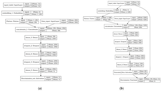
Figure 1. The architecture of K-CGAN: (a) K-CGAN Discriminator Architecture; (b) K-CGAN Generator Architecture with Novelty Loss.

The generator $\mathrm{G}$ and discriminator $\mathrm{D}$ in the K-CGAN are continually at odds with one another. The discriminator is meant to be confused with the generator. It is the responsibility of the discriminator to separate the events generated by the generator from those in the supplied dataset. The generator’s data will be of low quality if the discriminator has no trouble determining which instances came from it. Consider the K-CGAN setup as the generator’s training ground. The discriminator instructs the generator’s evolution and provides feedback on the instances it generates. The objective function of our proposed K-CGAN is defined as follows:

$$\mathrm{JD}=-\frac{1}{2\mathrm{m}}{\displaystyle \sum }_{\mathrm{i}=1}^{\mathrm{m}}{=\mathrm{logD}(\mathrm{x}}_{\mathrm{i}}{,\mathrm{y}}_{\mathrm{i}})+{\displaystyle \sum }_{\mathrm{i}=1}^{\mathrm{m}}{\log (1-\mathrm{D}(\mathrm{G}(\mathrm{z}}_{\mathrm{i}}{,\mathrm{y}}_{\mathrm{i}}{),\mathrm{y}}_{\mathrm{i}}\left)\right)$$

(18)

The CGAN training procedure is remarkably similar to that of the original GAN. The logistic cost function for the gradient is obtained by feeding a mini batch of $\mathrm{m}$ training samples $\left({\mathrm{x}}_{\mathrm{i}},{\mathrm{y}}_{\mathrm{i}}\right){\mathrm{m}}_{\mathrm{i}}=1$ and $\mathrm{m}$ noise random samples ${\mathrm{z}}_{\mathrm{i}}{\mathrm{m}}_{\mathrm{i}}=1$. In order to trick the discriminator into categorizing the data set and create it as the training dataset, the generator seeks to provide data that are relatively close to the training set.

4.1. Generator Loss

The role of the generator in K-CGAN is to produce synthetic samples to fool the discriminator and make the discriminator think the samples are real or fake. The proposed K-CGAN method has a new loss element which is based on KL divergence. In this method, the generator loss has two main tasks. First, to fool the discriminator and for that this study used binary cross entropy. The second task of the generator loss is to ensure that the synthetic data distribution is similar to that of the Original Data distribution and for that this study used KL divergence. This equation presents the tasks of generator loss (trained binary cross entropy and KL divergence). The task of KL divergence is to measure the expected number of bits needed to code samples from p(x) when using a code on the basis of q(x). Generally, p(x) denotes the true distribution of data. On the other hand, q(x) typically signifies a description, model, theory, or approximation of p(x). Here, p(x) and q(x) are probability distributions of a random variable x. The sum of both these random variables is 1. Furthermore, p(x) and q(x) are greater than 0 while the function of binary cross entropy is to compare predicted probabilities to an actual class output that can be 0 or 1. Binary cross entropy then calculates the score that penalizes the probabilities on the basis of the distance from the expected value, thus, calculating how far or close it is from the actual value. The binary cross entropy loss function estimates the average cross entropy of all examples, where y denotes the class label, and “ŷ_i” denotes the predicted probability of the data for all N data points.

$$\mathrm{Loss}=-\frac{1}{\mathrm{output}\mathrm{size}}{{\displaystyle \sum }}_{\mathrm{i}=1}^{\mathrm{output}\mathrm{size}}\mathrm{Yi}\times \log \mathsf{ŷ}\mathrm{i}+(1-\mathsf{ŷ}\mathrm{i})\times \log (1-\mathsf{ŷ}\mathrm{i})+{\displaystyle \sum }\mathrm{pi}\left(\mathrm{x}\right)\log (\frac{\mathrm{pi}\left(\mathrm{x}\right)}{\mathrm{qi}\left(\mathrm{x}\right)})$$

(19)

The characteristics of our custom generator loss and specific best performing hyperparameter settings have produced an improved performance which is evident in the classifiers performance results and data samples produced by the model which resemble the original credit card fraud dataset.

4.2. Discriminator Loss

The responsibility of the discriminator is to increase the possibility that the sample exhibits accurate data traits and decreases the possibility of falsified data. The binary cross entropy loss function estimates the average cross entropy of all examples. The equation below represents the discriminator loss. Where y denotes the class label, and “ŷ_i” denotes the predicted probability of the data for all N data points.

$$\mathrm{Loss}=-\frac{1}{\mathrm{output}\mathrm{size}}{\displaystyle \sum }_{\mathrm{i}=1}^{\mathrm{output}\mathrm{size}}{\mathrm{Y}}_{\mathrm{i}}\times \log {\mathsf{ŷ}}_{\mathrm{i}}+(1- {\mathsf{ŷ}}_{\mathrm{i}})\times \log (1-{\mathsf{ŷ}}_{\mathrm{i}})$$

(20)

5. Experiments

This section of the current study provides a high-level overview of the methodologies employed in the course of this investigation. Further, the procedure itself is described here.

5.1. Dataset

Researchers in the field of credit card transactions face a number of challenges, one of the most significant being the lack of real-world data due to data privacy and sensitivity considerations. Therefore, the publicly available Credit Card Fraud detection database downloaded from Kaggle [6,31] as used for this investigation. Further details about the dataset are presented in Table 1, Table 2 and Table 3.

Table 1. Credit card dataset (sourced from Kaggle.com).

Dataset	No. of Attributes	No. of Instances	No. of Fraud Instances	No. of Legal Instances
Kaggle	30	31	492	284,315

Table 2. Credit card dataset features (highlighted in bold) (first samples of rows).

Time	V1	V2	V3	V4	V5	V6	V7	V8
0	−1.35981	−0.07278	2.536347	1.378155	−0.33832	0.462388	0.239599	0.098698
0	1.191857	0.266151	0.16648	0.448154	0.060018	−0.08236	−0.0788	0.085102
1	−1.35835	−1.34016	1.773209	0.37978	−0.5032	1.800499	0.791461	0.247676
1	−0.96627	−0.18523	1.792993	−0.86329	−0.01031	1.247203	0.237609	0.377436
2	−1.15823	0.877737	1.548718	0.403034	−0.40719	0.095921	0.592941	−0.27053
2	−0.42597	0.960523	1.141109	−0.16825	0.420987	−0.02973	0.476201	0.260314
4	1.229658	0.141004	0.045371	1.202613	0.191881	0.272708	−0.00516	0.081213
7	−0.64427	1.417964	1.07438	−0.4922	0.948934	0.428118	1.120631	−3.80786
7	−0.89429	0.286157	−0.11319	−0.27153	2.669599	3.721818	0.370145	0.851084
V9	V10	V11	V12	V13	V14	V15	V16	V17
0.363787	0.090794	−0.5516	−0.6178	−0.99139	−0.31117	1.468177	−0.4704	0.207971
−0.25543	−0.16697	1.612727	1.065235	0.489095	−0.14377	0.635558	0.463917	−0.1148
−1.51465	0.207643	0.624501	0.066084	0.717293	−0.16595	2.345865	−2.89008	1.109969
−1.38702	−0.05495	−0.22649	0.178228	0.507757	−0.28792	−0.63142	−1.05965	−0.68409
0.817739	0.753074	−0.82284	0.538196	1.345852	−1.11967	0.175121	−0.45145	−0.23703
−0.56867	−0.37141	1.341262	0.359894	−0.35809	−0.13713	0.517617	0.401726	−0.05813
0.46496	−0.09925	−1.41691	−0.15383	−0.75106	0.167372	0.050144	−0.44359	0.002821
0.615375	1.249376	−0.61947	0.291474	1.757964	−1.32387	0.686133	−0.07613	−1.22213
−0.39205	−0.41043	−0.70512	−0.11045	−0.28625	0.074355	−0.32878	−0.21008	−0.49977
V18	V19	V20	V21	V22	V23	V24	V25	V26
0.025791	0.403993	0.251412	−0.01831	0.277838	−0.11047	0.066928	0.128539	−0.18911
−0.18336	−0.14578	−0.06908	−0.22578	−0.63867	0.101288	−0.33985	0.16717	0.125895
−0.12136	−2.26186	0.52498	0.247998	0.771679	0.909412	−0.68928	−0.32764	−0.1391
1.965775	−1.23262	−0.20804	−0.1083	0.005274	−0.19032	−1.17558	0.647376	−0.22193
−0.03819	0.803487	0.408542	−0.00943	0.798278	−0.13746	0.141267	−0.20601	0.502292
0.068653	−0.03319	0.084968	−0.20825	−0.55982	−0.0264	−0.37143	−0.23279	0.105915
−0.61199	−0.04558	−0.21963	−0.16772	−0.27071	−0.1541	−0.78006	0.750137	−0.25724
−0.35822	0.324505	−0.15674	1.943465	−1.01545	0.057504	−0.64971	−0.41527	−0.05163
0.118765	0.570328	0.052736	−0.07343	−0.26809	−0.20423	1.011592	0.373205	−0.38416
						V27	V28	Amount
						0.133558	−0.02105	149.62
						−0.00898	0.014724	2.69
						−0.05535	−0.05975	378.66
						0.062723	0.061458	123.5
						0.219422	0.215153	69.99
						0.253844	0.08108	3.67
						0.034507	0.005168	4.99
						−1.20692	−1.08534	40.8
						0.011747	0.142404	93.2

Table 3. Variance inflation factor (VIF).

Feature	VIF
Time	1.104214
V1	1.003973
V2	1.000397
V3	1.038927
V4	1.002805
V5	1.007125
V6	1.000983
V7	1.002670
V8	1.001018
V9	1.000367
V10	1.001049
V11	1.013779
V12	1.003927
V13	1.000932
V14	1.002786
V15	1.007373
V16	1.000528
V17	1.002051
V18	1.002158
V19	1.000196
V20	1.000669
V21	1.001252
V22	1.004694
V23	1.000729
V24	1.000058
V25	1.012106
V26	1.000409
V27	1.000941
V28	1.000440
Amount	11.650240

The dataset includes credit card transactions made in September 2013 throughout Europe. Within this dataset, a two-day period contains 492 fraudulent transactions out of a total of 284,315 transactions with 30 attributes. The dataset is severely unbalanced, with only 0.172% of all transactions representing true positives (frauds).

In addition, these data have 31 numerical features. Furthermore, the input variables had financial details, so the PCA transformation was made for the input variables to maintain anonymity of the data. Out of the total features, only three were kept original. The non-numerical feature ‘Time’ indicates the time between the initial activity via credit card and all other activities. The feature ‘Amount’ represents the transaction amount made using credit card, and the feature ‘Class’ shows the label, and there are only two values: 0 for legal transactions and 1 for fraud transactions. Variance inflation factor (VIF) are presented in Table 3.

5.2. Division of Dataset

The research study provides the classification of credit card fraud using all of the available oversampling techniques and classification algorithms after 100 epochs. Using the data collected, a different training set and test set were produced. Eighty percent of the data from each class were included in the training set, whereas only twenty percent were included in the test set.

5.3. Hyperparameters

K-CGAN

In GAN-based architectures, the discriminator is trained to differentiate between real and generated samples. On the other hand, the generator competes with the discriminator or produces artificial data samples. Table 4 and Table 5 present the discriminator and the generator hyper parameters for a K-CGAN neural network. Further supplementary Table 6 and Table 7 represent Vanilla GAN hyperparameter settings.

Table 4. K-CGAN Generator Neural Network Hyperparameter Settings.

Parameter	Value
Learning Rate	0.0001
Hidden Layer Optimizer	Relu
Output Optimizer	Adam
Loss Function	Trained Discriminator Loss+ KL Divergence
Hidden Layers	2, −128, 64
Dropout	0.1
Random Noise Vector	100
Kernel Initializer	glorot_uniform
Kernel Regularizer	L2 method
Total Learning Parameters	36,837

Table 5. K-CGAN Discriminator Neural Network Hyperparameter Settings.

Parameter	Value
Learning Rate	0.0001
Hidden Layer Optimizer	LeakyRelu
Output Optimizer	Adam
Loss Function	Binary Cross Entropy
Hidden Layers	2, −20, 10
Dropout	0.1
Kernel Regularizer	L2 method

Table 6. GAN Generator Neural Network Hyperparameter Settings.

Parameter	Value
Learning Rate	0.0001
Hidden Layer Optimizer	Relu
Output Optimizer	RMSprop
Loss Function	Trained Discriminator Loss
Hidden Layers	64, 32
Dropout	0.5
Random Noise Vector	100

Table 7. GAN Discriminator Neural Network Hyperparameter Settings.

Parameter	Value
Learning Rate	0.0001
Hidden Layer Optimizer	LeakyRelu
Output Optimizer	RMSprop
Loss Function	Binary Cross Entropy
Hidden Layers	128, 64, 32
Dropout	0.1

6. Results Analysis

This section presents a detailed comparison of the experiments conducted to address the imbalanced class challenge in the credit card-based fraud detection dataset. This part of the paper also offers a comparative study on techniques on the classifiers, such as XG-Boost, Random Forest, Nearest Neighbor, MLP, and Logistic Regression. Furthermore, we have also discussed and explained the results of our experimental study in the form of various graphs and tables.

Evaluation of Classification Models

This section presents a detailed comparison of different classification methods in terms of performance indicators. The performance indicators are Precision, Recall, F1 Score, and Accuracy. In this section, we have presented an evaluation of the classification models in tabular representation. The results in Table 8, Table 9, Table 10, Table 11 and Table 12 illustrate the classification performance of a balanced dataset that includes synthesized minority class samples from each technique: K-CGAN, SMOTE, ADASYN, B-SMOTE, Vanilla GAN, WS GAN, SDG GAN, NS GAN, and LS GAN. When these samples are merged with an imbalanced dataset it creates balance overall. We are also including classifiers’ performance against the ‘Original Dataset’ which represents a classifier’s performance against an original imbalanced dataset. The augmented sample size has a strong influence on the performance of the classifiers used in this research. As shown in Table 10, when increasing the augmented sample size from 492 to synthetizing an additional 283,823 fraud transactions which creates an equal ratio of minority and majority classes (284,315 valid and 284,315 fraud transactions), there is an increase in the F1 Score from 0.87 to 0.99 for XG-Boost, from 0.86 to 0.99 for Random Forest and MLP, 0.78 to 0.99 for Nearest Neighbor, and 0.72 to 0.99 for Logistic Regression. There was also an increase in Precision, Accuracy, and Recall, which is presented in Table 8, Table 9, Table 10 and Table 11. We have also tested classifiers’ performance against K-CGAN synthetic data only and Table 12 demonstrates the results (sample of 30,000 valid and 30,000 fraud transactions generated by K-CGAN model) demonstrating that increasing the augmented sample size also leads to an increase in F1 Score, Precision, Recall, and Accuracy scores for each classifier used in this research. All five classifiers saw increases in scores when their corresponding augmented sample sizes increased. This further underlines the importance of having a larger sample size when creating a classification model.

Table 8. Precision values for classification methods for balanced dataset.

	Precision Value for Balanced Dataset
	K-CGAN	Original Dataset	SMOTE	ADASYN	B-SMOTE	Vanilla GAN	WS GAN	SDG GAN	NS GAN	LS GAN
XG-Boost	0.999762	0.924370	0.999467	0.999182	0.999816	0.997085	0.988636	0.986072	0.980831	0.982405
Random Forest	0.999776	0.931035	0.999762	0.999760	0.999958	0.994135	0.980170	0.986111	0.977564	0.982249
Nearest Neighbor	0.999608	0.864865	0.982366	0.973762	0.997603	0.960606	0.954416	0.966197	0.954545	0.961194
MLP	0.999692	0.881890	0.997690	0.997970	0.998082	0.982456	0.974504	0.957219	0.962145	0.959885
Logistic Regression	0.999566	0.890110	0.974443	0.909084	0.994725	0.965732	0.958457	0.970149	0.949495	0.968051

Table 9. Recall values for classification methods for balanced dataset.

	Recall Value for Balanced Dataset
	K-CGAN	Original Dataset	SMOTE	ADASYN	B-SMOTE	Vanilla GAN	WS GAN	SDG GAN	NS GAN	LS GAN
XG-Boost	0.999706	0.827068	1.000000	0.999986	0.999703	0.955307	0.932976	0.917098	0.962382	0.941011
Random Forest	0.999706	0.812030	1.000000	1.000000	0.999661	0.946927	0.927614	0.919689	0.956113	0.932584
Nearest Neighbor	0.999706	0.721804	0.999804	1.000000	0.999746	0.885475	0.898123	0.888601	0.921630	0.904494
MLP	0.999594	0.842105	1.000000	0.999929	0.999746	0.938547	0.922252	0.927461	0.956113	0.941011
Logistic Regression	0.999608	0.609023	0.919681	0.860942	0.996383	0.865922	0.865952	0.841969	0.884013	0.851124

Table 10. F1 Score values for classification methods.

	F1 Score Value for Balanced Dataset
	K-CGAN	Original Dataset	SMOTE	ADASYN	B-SMOTE	Vanilla GAN	WS GAN	SDG GAN	NS GAN	LS GAN
XG-Boost	0.999734	0.873016	0.999733	0.999584	0.999760	0.975749	0.960000	0.950336	0.971519	0.961263
Random Forest	0.999741	0.867470	0.999881	0.999880	0.999809	0.969957	0.953168	0.951743	0.966720	0.956772
Nearest Neighbor	0.999657	0.786885	0.991008	0.986707	0.998673	0.921512	0.925414	0.925776	0.937799	0.931983
MLP	0.999643	0.861538	0.998844	0.998949	0.998913	0.960000	0.947658	0.942105	0.959119	0.950355
Logistic Regression	0.999587	0.723214	0.946270	0.884358	0.995553	0.913108	0.909859	0.901526	0.915584	0.905830

Table 11. Accuracy values for classification methods.

	Accuracy Value for Balanced Dataset
	K-CGAN	Original Dataset	SMOTE	ADASYN	B-SMOTE	Vanilla GAN	WS GAN	SDG GAN	NS GAN	LS GAN
XG-Boost	0.999733	0.999551	0.999733	0.999585	0.999761	0.999762	0.999594	0.999482	0.999748	0.999622
Random Forest	0.999740	0.999537	0.999880	0.999880	0.999810	0.999706	0.999524	0.999496	0.999706	0.999580
Nearest Neighbor	0.999655	0.999270	0.990905	0.986578	0.998678	0.999244	0.999244	0.999230	0.999454	0.999342
MLP	0.999641	0.999494	0.998839	0.998952	0.998917	0.999608	0.999468	0.999384	0.999636	0.999510
Logistic Regression	0.999585	0.999129	0.947643	0.887842	0.995568	0.999174	0.999104	0.999006	0.999272	0.999118

Table 12. Comparison of classification models using the K-CGAN synthetic data only (sample of 30,000 valid and 30,000 fraud transactions generated by K-CGAN model).

Algorithm	Precision	Recall	F1 Score	Accuracy
XG-Boost	1.0	1.000000	1.000000	1.00000
Random Forest	1.0	0.982301	0.991071	0.99996
Nearest Neighbor	1.0	0.929204	0.963303	0.99984
MLP	1.0	1.000000	1.000000	1.00000
Logistic Regression	1.0	0.946903	0.972727	0.99988

In Table 8 below, this paper presents the Precision of classifiers for imbalance class methods. Among the classification methods, K-CGAN, SMOTE, and B-SMOTE performed better when compared with other methods. Among the classifiers, XG-Boost and Random Forest achieved better results.

In Table 9 below, this paper presents the Precision of classifiers for imbalance class methods. Among the classification methods, K-CGAN, SMOTE, and ADASYN performed better when compared with other methods. Among the classifiers, XG-Boost and Random Forest achieved better results.

In Table 10 below, this paper presents the F1 Score values of classification methods. Among the classification methods K-CGAN, B-SMOTE performed better when compared with other methods. Among classifiers XG-Boost, MLP and Random Forest achieved better results.

In the below Table 11, this paper presents the Accuracy of classifiers for imbalance class methods. Among the classification methods K-CGAN, NS GAN, Vanilla GAN performed better when compared with other methods. Among classifiers XG-Boost and Random Forest achieved better results.

Among all the classification methods KC-GAN performed very well on all classifiers. Apart from that, SMOTE, ADASYN, B-SMOTE, Vanilla GAN performed effectively as well.

Furthermore, Table 12 presents the results of K-CGAN based synthetic data only. The result shows that XG-Boost has Precision (1.0), Recall (1.000000), F1 Score (1.000000), and Accuracy (1.00000) values. However, Random Forest has Precision (1.0), Recall (0.982301), F1 Score (0.991071), and Accuracy (0.99996) values. Further, the result shows that Nearest Neighbor has Precision (1.0), Recall (0.929204), F1 Score (0.963303), and Accuracy (0.99984) values. However, MLP has Precision (1.0), Recall (1.000000), F1 Score (1.000000), and Accuracy (1.00000) values. Furthermore, Logistic Regression has Precision (1.0), Recall (0.946903), F1 Score (0.972727), and Accuracy (0.99988) values. Among the classifiers XG-Boost and MLP achieved maximum scores in terms of Precision, Recall, F1 Score, and Accuracy, while Random Forest also achieved good scores.

The F1 Score, Recall, Accuracy, and Precision measures are metrics which are used in classification models [26]. Accuracy measures the number of predictions which are correct as a percentage of the total number of predictions that are made. For instance, if 80% of our predictions are correct, then our Accuracy will be 80%. It is effective only when the distribution of classes is equal in our classification. The Precision metric counts the percentage that is correct. This metric does not always find all the positives, but whenever it finds a positive, they are likely to be correct. Furthermore, a model with a high Recall rate succeeds well in finding positive cases in the dataset. Conversely, a model with a low Recall rate is unable to find all of the positive cases present in the data. Furthermore, the other common metrics are Recall and Precision which takes imbalanced class into account. On the other hand, in F1 Score we calculate the average of Recall and Precision. In other words, the F1 Score combines both the Recall and Precision into a single metric. Figure 2, Figure 3, Figure 4, Figure 5, Figure 6, Figure 7, Figure 8, Figure 9, Figure 10, Figure 11 and Figure 12 exhibit the ROC curves for each classification method along with the imbalance class techniques used in this study. For each method, the performance of the classifier is demonstrated. The below graphs are self-explanatory and we can easily judge the performance of each classifier for all machine learning algorithms used in this paper. ROC curve visualizations are commonly used when assessing model performance in binary classification problems, as it can provide insight into how well a given classification system is able to distinguish between two classes. ROC curves are also used to compare different models and determine which one offers the best classification Accuracy.

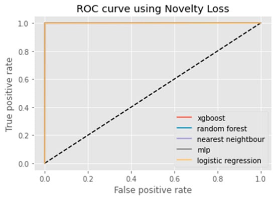
Figure 2. ROC curve of K-CGAN.

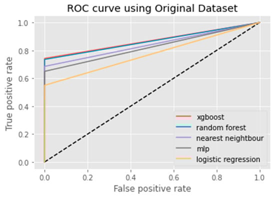
Figure 3. ROC curve of Original Dataset.

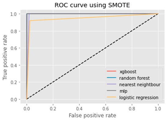
Figure 4. ROC curve using SMOTE.

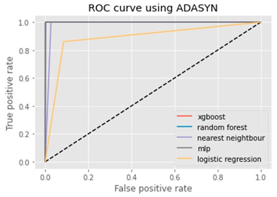
Figure 5. ROC curve using ADASYN.

Figure 6. ROC curve using B-SMOTE.

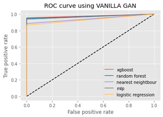
Figure 7. ROC curve using Vanilla GAN.

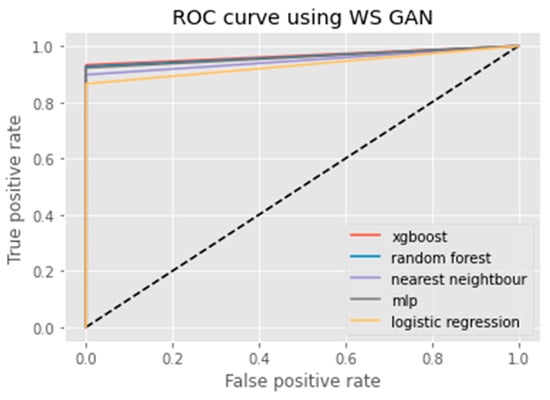
Figure 8. ROC curve using WS GAN.

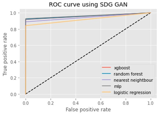
Figure 9. ROC curve using SDG GAN.

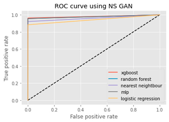
Figure 10. ROC curve using NS GAN.

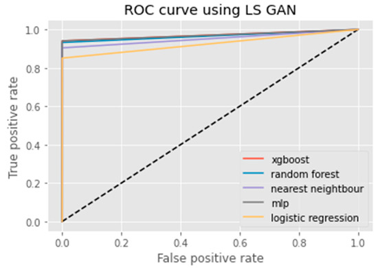
Figure 11. ROC curve using LS GAN.

Figure 12. ROC curve using K-CGAN.

An ROC curve (receiver operating characteristic curve) is a graphical representation of the false positive rate (FPR) of a given classification system. The FPR is calculated by dividing the number of false positives by the total number of results returned in a test set. The x-axis on an ROC plot typically represents the false positive rate (FPR), while the y-axis represents the true positive rate (TPR). An ROC curve is a useful tool for assessing model performance as it can help to determine whether a given classification system has high Accuracy and low bias. The farther away from the diagonal line on an ROC plot, the higher the Accuracy of the model. A perfect classifier would have a TPR of 1 and an FPR of 0, which is represented in the top-left corner of the plot.

Correlation comparison is an important part of data analysis. Using correlation comparison, we can compare the relationship between the groups of variables. Correlation comparison allows us to determine whether there is a positive or negative relationship between these variables and to identify any patterns or trends in the data. By understanding these relationships, we are able to develop more effective data augmentation and pre-processing techniques for improving machine learning performance.

As shown in Figure 13, the relationships between different variables show that Novelty K-CGAN, SMOTE, ADASYN, and B-SMOTE are more similar to the Original Dataset than other methods. On the other hand, Vanilla GAN, WS GAN, SDG GAN, NS GAN, and LS GAN are less similar to the Original Dataset, which suggests that these models may not be suitable for this dataset. Furthermore, we can observe that K-CGAN has a higher correlation than other methods as it does not introduce any bias or noise in the data. This confirms our method is suitable for the respective Credit Card Fraud Dataset and demonstrates the effectiveness of K-CGAN at preserving the structure of the Original Dataset.

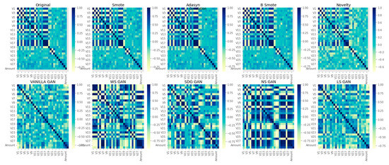
Figure 13. Correlation comparison of Original Data, SMOTE, ADASYN, B-SMOTE, Novelty K-CGAN, Vanilla GAN, WS GAN, SDG GAN, NS GAN, and LS GAN methods.

We have adopted univariate distribution for summarizing the data and understanding their distribution across different groups or categories. It is useful for gaining data insights and in identifying any outliers or unusual features within the data. As per Figure 14, Figure 15 and Figure 16, the univariate distribution demonstrates that K-CGAN resembles the Original Data closely. The distance between the actual and generated samples is less in the case of K-CGAN compared with other GAN-based algorithms.

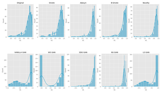
Figure 14. Univariate V1 Feature Distribution comparison of Original Data, Smote, ADASYN, B-SMOTE, Novelty K-CGAN, Vanilla GAN, WS GAN, SDG GAN, NS GAN, and LS GAN methods.

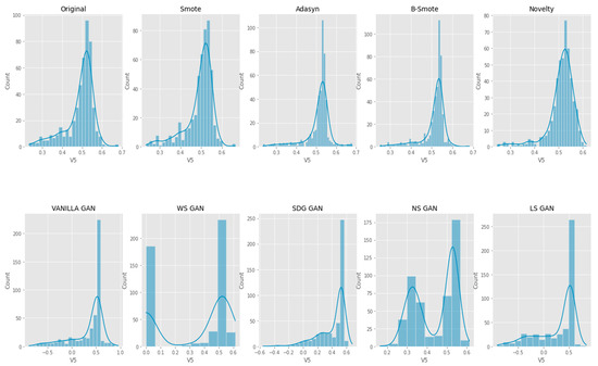
Figure 15. Univariate V5 Feature Distribution comparison of Original Data, SMOTE, ADAYSN, B-SMOTE, Novelty K-CGAN, Vanilla GAN, WS GAN, SDG GAN, NS GAN, and LS GAN methods.

Figure 16. Univariate V15 Feature Distribution comparison of Original Data, SMOTE, ADAYSN, B-SMOTE, Novelty K-CGAN, Vanilla GAN, WS GAN, SDG GAN, NS GAN, and LS GAN methods.

Bivariate visualization is a type of data analysis that can be used to evaluate relationships between two variables. It is a powerful tool to understand the correlation between two different sets of data. The visualization helps in identifying patterns and correlations quickly, which can be used for further analysis or for making decisions. Bivariate visualization can be used to compare two different variables. The data points generated by the K-CGAN resemble the original data samples, as can be seen from the visualizations (Figure 17, Figure 18 and Figure 19). Bivariate visualization charts of data points generated by K-CGAN showed high agreement with the original dataset.

Figure 17. Bivariate V1 vs V3 Feature Distribution comparison of Original Data, SMOTE, ADAYSN, B-SMOTE, Novelty K-CGAN, Vanilla GAN, WS GAN, SDG GAN, NS GAN, and LS GAN methods.

Figure 18. Bivariate V1 vs V4 Feature Distribution comparison of Original Data, SMOTE, ADAYSN, B-SMOTE, Novelty K-CGAN, Vanilla GAN, WS GAN, SDG GAN, NS GAN, and LS GAN methods.

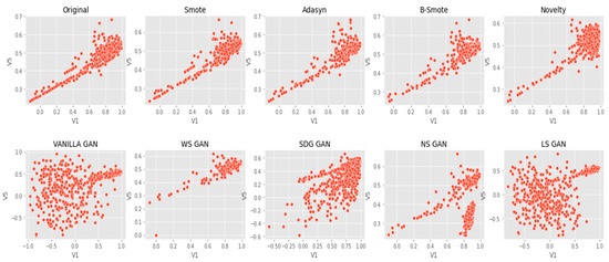
Figure 19. Bivariate V1 vs. V5 Feature Distribution comparison of Original Data, SMOTE, ADASYN, B-SMOTE, Novelty K-CGAN, Vanilla GAN, WS GAN, SDG GAN, NS GAN, and LS GAN methods.

7. Conclusions

Due to recent technical advancements, credit cards have become more widely used as a practical payment mechanism. Businesses lose millions of dollars each year to an expanding fraud phase as a result of inadequate security measures. An extensive strategy that includes both detection and prevention actions is required to lower the prevalence of credit card theft. The main goal of this research is to contrast and compare the classifiers’ skills and results in differentiating between fraudulent and lawful transactions. The current study also aims to examine the effectiveness of various resampling approaches in improving the classification outputs of the classification models and to assess the models’ ability to discriminate between fraudulent and legitimate transactions. It is important to note that the results of all the classifiers varied. The Precision, Recall, F1 Score, and Accuracy are used to assess effectiveness. The result shows that B-SMOTE, K-CGANs, and SMOTE have the highest Precision and Recall when compared with other resampling methods. Further, the result shows that our novel method K-CGAN has the highest F1 Score and Accuracy when compared with other resampling methods. Furthermore, the data points generated by the K-CGAN resemble the original data samples, as can be seen from the visualizations. This reveals the potential of K-CGAN to effectively learn from real data, and accurately generate new samples that are indistinguishable from the original ones. The results also demonstrate K-CGAN’s ability to capture the underlying structure and features of the data in a high-dimensional space. This is an important step towards creating realistic data samples.

References

- Asha, R.; Suresh, K. Credit card fraud detection using an artificial neural network. Glob. Transit. Proc. 2021, 2, 35–41. [Google Scholar]
- Garg, V.; Chaudhary, S.; Mishra, A. Analyzing Auto ML Model for Credit Card Fraud Detection. Int. J. Innov. Res. Comput. Sci. Technol. (IJIRCST) ISSN 2021, 9, 2347–5552. [Google Scholar]
- Alejo, R.; García, V.; Marqués, A.I.; Sánchez, J.S.; Antonio-Velázquez, J.A. Making accurate credit risk predictions with cost-sensitive mlp neural networks. In Management Intelligent Systems; Springer: Heidelberg, Germany, 2013; pp. 1–8. [Google Scholar]
- Sanober, S.; Alam, I.; Pande, S.; Arslan, F.; Rane, K.P.; Singh, B.K.; Khamparia, A.; Shabaz, M. An enhanced secure deep learning algorithm for fraud detection in wireless communication. Wirel. Commun. Mob. Comput. 2021, 2021, 6079582. [Google Scholar] [CrossRef]
- Xue, W.; Zhang, J. Dealing with imbalanced dataset: A re-sampling method based on the improved SMOTE algorithm. Commun. Stat. Simul. Comput. 2013, 45, 1160–1172. [Google Scholar] [CrossRef]
- Hajek, P.; Abedin, M.Z.; Sivarajah, U. Fraud Detection in Mobile Payment Systems using an XGBoost-based Framework. Inf. Syst. Front. 2022, 1–19. [Google Scholar] [CrossRef] [PubMed]
- Jiang, C.; Song, J.; Liu, G.; Zheng, L.; Luan, W. Credit card fraud detection: A novel approach using aggregation strategy and feedback mechanism. IEEE Internet Things J. 2018, 5, 3637–3647. [Google Scholar] [CrossRef]
- Makki, S.; Assaghir, Z.; Taher, Y.; Haque, R.; Hacid, M.S.; Zeineddine, H. An experimental study with imbalanced classification approaches for credit card fraud detection. IEEE Access 2019, 7, 93010–93022. [Google Scholar] [CrossRef]
- Wang, T.; Zhao, Y. Credit Card Fraud Detection using Logistic Regression. In Proceedings of the 2022 International Conference on Big Data, Information and Computer Network (BDICN), Sanya, China, 20–22 January 2022; pp. 301–305. [Google Scholar]
- Goodfellow, I.; Pouget-Abadie, J.; Mirza, M.; Xu, B.; Warde-Farley, D.; Ozair, S.; Courville, A.; Bengio, Y. Generative adversarial networks. Commun. ACM 2020, 63, 139–144. [Google Scholar] [CrossRef]
- Charitou, C.; Dragicevic, S.; Garcez, A.D.A. Synthetic Data Generation for Fraud Detection using GANs. arXiv 2021, arXiv:2109.12546. [Google Scholar]
- Chen, J.; Shen, Y.; Ali, R. Credit card fraud detection using sparse autoencoder and generative adversarial network. In Proceedings of the 2018 IEEE 9th Annual Information Technology, Electronics and Mobile Communication Conference (IEMCON), Vancouver, BC, Canada, 1–3 November 2018; pp. 1054–1059. [Google Scholar]
- Ngwenduna, K.S.; Mbuvha, R. Alleviating class imbalance in actuarial applications using generative adversarial networks. Risks 2021, 9, 49. [Google Scholar] [CrossRef]
- Paasch, C.A. Credit Card Fraud Detection Using Artificial Neural Networks Tuned by Genetic Algorithms; Hong Kong University of Science and Technology: Hong Kong, China, 2008. [Google Scholar]
- Kumar, P.; Iqbal, F. Credit card fraud identification using machine learning approaches. In Proceedings of the 2019 1st International conference on innovations in information and communication technology (ICIICT), Chennai, India, 25–26 April 2019; pp. 1–4. [Google Scholar]
- Lamba, H. Credit Card Fraud Detection in Real-Time. Ph.D. Thesis, California State University San Marcos, San Marcos, CA, USA, 2020. [Google Scholar]
- Chen, X.W.; Wasikowski, M. Fast: A roc-based feature selection metric for small samples and imbalanced data classification problems. In Proceedings of the 14th ACM SIGKDD International Conference on Knowledge Discovery and Data Mining, Las Vegas, NV, USA, 24–27 August 2008; pp. 124–132. [Google Scholar]
- Prusti, D.; Rath, S.K. Web service based credit card fraud detection by applying machine learning techniques. In Proceedings of the TENCON 2019-2019 IEEE Region 10 Conference (TENCON), Kochi, India, 17–20 October 2019; pp. 492–497. [Google Scholar]
- Zheng, Y.J.; Zhou, X.H.; Sheng, W.G.; Xue, Y.; Chen, S.Y. Generative adversarial network-based telecom fraud detection at the receiving bank. Neural Netw. 2018, 102, 78–86. [Google Scholar] [CrossRef] [PubMed]
- Singh, A.; Ranjan, R.K.; Tiwari, A. Credit card fraud detection under extreme imbalanced data: A comparative study of data-level algorithms. J. Exp. Theor. Artif. Intell. 2022, 34, 571–598. [Google Scholar] [CrossRef]
- Sadgali, I.; Nawal, S.A.E.L.; Benabbou, F. Fraud detection in credit card transaction using machine learning techniques. In Proceedings of the 2019 1st International Conference on Smart Systems and Data Science (ICSSD), Rabat, Morocco, 3–4 October 2019; pp. 1–4. [Google Scholar]
- Sethia, A.; Patel, R.; Raut, P. Data augmentation using generative models for credit card fraud detection. In Proceedings of the 2018 4th International Conference on Computing Communication and Automation (ICCCA), Greater Noida, India, 14–15 December 2018; pp. 1–6. [Google Scholar]
- Ullah, I.; Mahmoud, Q.H. Design and development of a deep learning-based model for anomaly detection in IoT networks. IEEE Access 2021, 9, 103906–103926. [Google Scholar] [CrossRef]
- Omar, B.; Rustam, F.; Mehmood, A.; Choi, G.S. Minimizing the overlapping degree to improve class-imbalanced learning under sparse feature selection: Application to fraud detection. IEEE Access 2021, 9, 28101–28110. [Google Scholar]
- Li, J.; Zhu, Q.; Wu, Q.; Fan, Z. A novel oversampling technique for class-imbalanced learning based on SMOTE and natural neighbours. Inf. Sci. 2021, 565, 438–455. [Google Scholar] [CrossRef]
- Grandini, M.; Bagli, E.; Visani, G. Metrics for multi-class classification: An overview. arXiv 2020, arXiv:2008.05756. [Google Scholar]
- He, H.; Bai, Y.; Garcia, E.A.; Li, S. ADASYN: Adaptive synthetic sampling approach for imbalanced learning. In Proceedings of the 2008 IEEE International Joint Conference on Neural Networks (IEEE World Congress on Computational Intelligence), Hong Kong, 1–8 June 2008; pp. 1322–1328. [Google Scholar]
- Han, H.; Wang, W.Y.; Mao, B.H. August. Borderline-SMOTE: A new over-sampling method in imbalanced data sets learning. In International Conference on Intelligent Computing; Springer: Berlin/Heidelberg, Germany, 2005; pp. 878–887. [Google Scholar]
- Sohony, I.; Pratap, R.; Nambiar, U. Ensemble learning for credit card fraud detection. In Proceedings of the A.C.M. India Joint International Conference on Data Science and Management of Data, Goa, India, 11–13 January 2018; pp. 289–294. [Google Scholar]
- Taha, A.A.; Malebary, S.J. An intelligent approach to credit card fraud detection using an optimized light gradient boosting machine. IEEE Access 2020, 8, 25579–25587. [Google Scholar] [CrossRef]
- Kaggle.com. Available online: https://www.kaggle.com/mlg-ulb/creditcardfraud (accessed on 1 December 2022).
Disclaimer/Publisher’s Note: The statements, opinions and data contained in all publications are solely those of the individual author(s) and contributor(s) and not of MDPI and/or the editor(s). MDPI and/or the editor(s) disclaim responsibility for any injury to people or property resulting from any ideas, methods, instructions or products referred to in the content. |
© 2023 by the authors. Licensee MDPI, Basel, Switzerland. This article is an open access article distributed under the terms and conditions of the Creative Commons Attribution (CC BY) license (https://creativecommons.org/licenses/by/4.0/).