
A Time Window Analysis for Time-Critical Decision Systems with Applications on Sports Climbing

Research Group Biomechatronics, Ulm University of Applied Sciences, 89081 Ulm, Germany
*
Authors to whom correspondence should be addressed.
AI 2024, 5(1), 1-16; https://doi.org/10.3390/ai5010001
Submission received: 3 November 2023
/
Revised: 8 December 2023
/
Accepted: 13 December 2023
/
Published: 19 December 2023
Abstract
:Human monitoring systems are already utilized in various fields like assisted living, healthcare or sport and fitness. They are able to support in everyday life or act as a pre-warning system. We developed a system to monitor the ascent of a sport climber. It is integrated in a belay device. This paper presents the first time series analysis regarding the fall of a climber utilizing such a system. A Convolutional Neural Network handles the feature engineering part of the sensor information as well as the classification of the task at hand. In this way, the time is implicitly considered by the network. An analysis regarding the size of the time window was carried out with a focus on exploring the respective results. The neural network models were then tested against an already-existing principle based on a mechanical mechanism. We show that the size of the time window is a decisive factor in a time critical system. Depending on the size of the window, the mechanical principle was able to outperform the neural network. Nevertheless, most of our models outperformed the basic principle and returned promising results in predicting the fall of a climber within up to ms.
1. Introduction
Monitoring systems in sports have the ability to support the training progress of athletes, help in the recovery process after injuries or even prevent injuries from happening. In the domain of sport climbing, such a system can be externally placed or directly attached to the climber. External systems have the advantage of not interfering in any way with the climbers performance, although they often requires the installation of an additional setup prior to the ascent. Our monitoring system is directly integrated into a belay device from the Edelrid GmbH & Co. KG (Achener Weg 66, 88316 Isny im Allgäu) company, making it an external system which is directly involved with the climber through the rope. Additionally, no further equipment is required to set up when executing the climb.
With this device we are able to record the movement behavior of the belay device, and indirectly the climber’s movements, making it possible to keep track of the athlete’s performance. As it is directly integrated into the belay device, which is, among other devices, responsible for the safety of the climber, it can also be used to stop the rope that is running through the device. By stopping the rope in case of a fall situation, this can prevent a long fall and avert injuries or reduce the severity of injuries. Therefore, the time of identification is important. In addition to a project relevant context of having an onboard functionality to perform a user-specific update of the trainable network parameter, we decided to use a Convolutional Neural Network (CNN). The re-training of the network was faster than comparable networks based around Long Short-Term Memory cells or Gated Recurrent Units. A CNN network structure was enough to handle the temporal influence of the multisensor system regarding the classification task. In order to address the issue of fast identification, we analyzed several time windows to identify the fall of a climber as fast as possible, while still aiming for a low false positive rate. This is especially important to guarantee a high acceptance rate in the community of sport climbing. The CNN including the window approach has an advantage over standard machine learning approaches as it is able to take temporal influence into account.
So, the aim of this study was to analyze the effect of the size of the time window on the prediction result in a time-critical environment. Larger time windows tend to store more information for the predictive algorithm to increase the accuracy of the model. However, in a time-critical environment, the amount of time steps per window has to be kept at a minimum for a fast prediction. In summary, this study analyzes:
- The temporal influence of time windows in deep neural networks under the aspect of performing in a time critical environment.
- The environmental influences in the case of a fall whilst sport climbing, considering the time critical aspect of the fall itself.
- The importance of an AI-driven approach to handle the time critical aspect of identifying a fall in sport climbing.
In order to achieve this, we build a setup to simulate specifically predefined climb scenarios. These include ascents with varying behavior of climber and belayer and the falling of the climber into the rope. A measurement device was specifically developed to record the movement behavior of the belay device in those situations. The hardware system and the configurations are described in Section 3 alongside the processing of the raw data. The neural network architecture including the description of all relevant hyperparameter and settings is stated in Section 3.5. Finally, the results are structured in multiple parts in Section 4, where we begin with the overall classification quality. Then, we dive in deeper into the evaluation of the false positive rate and the identification time of the climbers falls.
2. Related Work
Monitoring systems are already used in multiple fields of sport, like rowing [1], running [2] or sport climbing [3]. They are used for different purposes such as to improve the training progress of the athletes [1,3], or to identify the performed activity [4,5]. Different sensor types were used in those studies to record biomechanical information. Those range from tracking the respiration of the lung [6,7], heart activity [7], eye gaze [8], muscle activity [9,10] and body movements [11,12]. An analysis about eye gaze in sport climbing was performed by Hacques et al. [8]. Especially in sport climbing, it is critical to coordinate the body movements according to the visual feedback. They were analyzing the effect of dealing with movement control in combination with the search for new movement possibilities. A different kind of analysis performed Balas et al. [6], as they focused on the respiratory information of the lungs to examine submaximal and maximal physiological responses whilst rock climbing and compare it with their skill level. Therefore, they recorded minute ventilation, oxygen uptake and carbon dioxide production using a calorimetry system attached to the climber throughout their ascent. The study group around Breen et al. [7] combined the respiratory minute ventilation information with information about the breathing and heart rate as well as the movement information of the hip. The sensors are integrated in the shirt of the athlete. Their aim is to use the sensor information to rate climbing strategies and training methods in order to improve the climbers performance. In particular, the recording of the movement information of the climber is often recorded to analyze climb typical activities. The sensors of choice are Inertial Measurement Units (IMUs). They are able to record accelerations and angular velocities. In some studies they rely on single IMUs, for example attached to the hip or an arm, or multiple IMUs placed on arms, legs and the chest of the climber. Ladha et al. [13] attached a single IMU on the wrist of the climber to record the movement throughout an ascent. Their aim was to develop a system for automatic coaching by relying on pre-defined assessment parameters like power, control, stability and speed. In contrast to the single IMU for performance measurement, Seifert et al. [14] equipped the climber with five IMU to monitor the performance of the athletes. The IMUs were placed on the feet, the forearms and on the pelvis. They were able to identify inappropriate rest positions caused by body–wall orientations. Another study by Bonfitto et al. [5] used an altimeter and accelerometer that were integrated into the harness of a climber to detect a climbers fall into the rope. Feature engineering was thereby performed manually on windows with a length of s and an overlap of s, and an artificial neural network was utilized to handle the task of fall identification.
Each of those systems containing an IMU has the ability to record the movement pattern of the climber. Our proposed system is not only able to implicitly monitor part of those movements, but also to monitor the belayer’s behavior as well. A previous study by Oppel et al. [15] showed the capability of the system by being able to differentiate between typical climbing movement patterns and the fall of a climber with the rope. Their study had the disadvantage of neglecting the temporal component and was not able to serve as a real-time system being able to intervene in the belaying system to support the belayer in case of an occurring fall. Therefore, the focus of this study is to include the previously missed temporal dependency to analyze the necessity of making it a real-time monitoring system.
3. Methods
This section provides an overview about the utilized hardware system to record the climbing and falling sequences and the methods to process and analyze the provided data for the machine learning pipeline.
3.1. Hardware System
The hardware system is described in detail in [15]. It is composed of two separate modules. One is attached to the harness of the climber and serves only to obtain the label information. The second module is integrated into the belay device of the belayer. Both include an MPU-9250 Inertial Measurement Unit (IMU) from the Infineon company to record their respective movement behavior, the ESP8266 WiFi module from the Espressif Systems company for communication and synchronisation purposes and an SD card to store the sensor information. The belay device is additionally equipped with three Infineon XSENSIVTM magnetic Hall switch TLE4945L sensors and six circularly arranged magnets with changing poles to record information about the rope running through the device. Both modules record the sensor information with Hz.
3.2. Data Configurations
Our study is about the identification of a climbers fall within typical climb specific activities. In order to handle this task, we adapted the problem to a two-class classification problem. Therefore, we separated the measurements in two parts. One to address the climb-specific activities and the other one to receive information about a climber’s fall. The setup for the falls was built around a sandbag serving as a substitute for the climber. In this way, falls of up to m were possible and it was necessary to identify the time of identification. Further information about the setup, as well as the conducting of the measurements can be found in [15].
The fall of a climber depends on a couple of influential factors regarding the duration, length and severity of the fall. In this article, we only address the first two parts and also neglect the influence of the climber’s deviation from the wall as well as their dynamic behavior whilst initiating the fall.
We recorded 161 falls with 19 different configurations, which are listed in Table 1. Most of the recordings were conducted whilst having no slack or fall potential in the system. However, in order to be able to obtain a general impression about the effectiveness of the prediction models in real climb situations, we varied the configurations for the two variables in the range from m to m. Additionally, the type of holding the device influences the movement behavior and, hence, the registered sensor information. With our recordings we address this issue by varying the way of holding the device.
3.3. Data Processing
Multiple processing steps were required to prepare the raw sensor information for the deep learning models. It starts with the unit transformation before the data is sequenced into different window sizes to address the time-critical aspect of the underlying task. Finally, the comparison model is introduced together with the network structure.
3.3.1. Data Acquisition and Filtering
The raw data from the sensors were recorded and stored on an SD-card. We extracted those information and at first converted them from digits into their respective physical units:
- for the acceleration signals;
- for the angular velocities;
- for rope distance.
A butterworth filter of 4th order with a cut-off frequency of Hz was then applied to remove high-frequency noise in the acceleration data. To remove the gravitational influence, we applied an AHRS algorithm [16]. This allowed us to rotate the IMU from a sensor-local to an earth-centered coordinate system and subtract the gravitational z-component.
3.3.2. Segmentation
The recordings contain information prior and posterior to the falls and climbing ascents. Therefore, we cut the respective sequences to the desired lengths. The identification of the starting point for the climb and fall sequences were identical. They were defined by the first timestamp registrating rope movement by using a threshold of m. From there, we allowed 25 additional samples prior to this timestamp. This timespan contains the movement information of the belay device before the rope is running through the device, see Figure 1. The final timestamp for the fall sequences was defined by the impact force. For the climb sequences, the end point was calculated based on the height information of the climber and the velocity of the rope. This allowed us to identify the time of lowering. Therefore, the rope had to reach a certain amount of distance and the velocity required to be zero for at least a second.
Climb sequences cover information about handing out rope and events without movement where the belayer just waits. Sequences of waiting, especially, resemble each other, as almost no activity is being recorded. This is why we divided the sequences into two categories, Moving and Waiting, see Figure 2.
The criteria for the subclass Moving are:
- Coherent time steps of a moving belay device with accelerations above and/or;
- Time steps where rope movement was registered.
In comparison are time steps that do not fulfill those requirements (white) and are therefore assigned to the class Waiting.
3.3.3. Windowing
In order to account for the temporal information, we further separated the segmented sequences by extracting shorter windows. The window sizes were specifically chosen to analyze the time critical system. The fastest recorded fall was 86 time steps long. Therefore, we set the limit of the window size to a maximum length of 80 time steps. In order to cover a broad spectrum of window sizes and their influence on the time critical system, we examined window sizes between 4 and 80 time steps long. Our final choice were window sizes of and 80. The step size for these windows was set to one for each fall and moving sequence within the climb class. Waiting sequences have a lower variance and are easier to distinguish from a climbers fall, so we set their step size to 5 time steps.
Events from the Moving subclass are temporally fast events which can occur in less than 80 time steps. In order to account for such fast events, we assigned each time window to this class if at least of consecutive time steps of the entire time window met one or more of the criteria to belong to the Moving subclass. However, this influences the relative fraction of the classes, see Figure 3. With an increasing window size, the total amount of samples within the classes Waiting and Fall decreased. The same is applicable for the relative quantity of the respective classes, as samples from the class Fall decreased from to , whereas the fraction of the subclass Waiting reduced from to . On the contrary, due to the method of processing, the amount of sequences from the Moving subclass increased with the window size. Its relative fraction changed from to . Over all windows, average and standard deviation of the classes are distributed as follows:
- of the samples belong to the class Fall;
- of the samples belong to the subclass Moving;
- of the samples belong to the subclass Waiting.
The input values are sensor-sensitive; hence, they are required to be scaled to reduce a sensor-specific influence whilst training. We applied the standard scaler onto the input data according to the following equation:
with being the i-th input sequence of the respective sensor, the average value per time step and sensor and the standard deviation per time step and sensor.
3.4. Comparison Model
In order to evaluate the performance of the deep learning models, we relied on a hard constraint. The idea is based on the Revo, an already-existing belay device from the Wild Country Ltd. Company (Derbyshire, UK). Their device blocks the rope movement through a mechanical mechanism. If the velocity of the rope reaches or higher, the device stops the movement. As we record the velocity of the rope, this feature serves as indicator for this hard constraint (HC-4 model). It is noteworthy that the HC-4 model does not include any information about the time, reducing the time sequence to one sample per window.
3.5. Machine Learning Pipeline
The machine learning pipeline is built around a four-fold hold-out cross-validation (cv). Each split is performed in a stratified manner, based on the recording level, meaning, from the 161 recorded falls and 45 ascents, each test set contains of those recordings in their full length. This allows for a recording based post analysis, comparable to utilizing the device in real-time. Within each cv-step, the training data is further split in a stratified manner, where of the data stays in the training set and is transferred to the validation set. In this way, each sequence is presented at least once for testing. To achieve comparable results, the identical sequences are presented within each cv-step for each time window model.
A CNN is used for training. Therefore, the weights are initialized anew in each cv-step and the structure of the CNN is kept the same. The complete network structure is visualized in Figure 4. The CNN layer is used to identify suitable features for the classifier. Additionally, 2D convolutions are applied in the time and feature domain, whereas a max-pooling layer reduces the feature space in the time domain solely. As the 2D convolutions are applied in the feature domain, the arrangement of the features have an influence on the outcome. We arrange them sensor-wise beginning with the accelerations, angular velocities and end with the rope distance. The axes of the individual 3-axis sensors are arranged by x, y and z. This leads to an input matrix for the network with the dimensions [batch size × window size × feature size], with a varying window size between 4 and 80 and a fixed feature size of 7. In order to handle overfitting, we rely on dropout and L2-regularization. The actual classifier consists of two hidden layer with 1024 and 256 neurons, respectively. As we split the climb class in two sub-classes, the output layer is comprised of three neurons. Within each hidden layer, we use the elu as the activation function, whereas the linear activation function is utilized for the CNN layer.
We use the basic stochastic gradient descent (SGD) algorithm without momentum as optimizer, with a learning rate of . The optimization process is performed over 1000 epochs and stopped with the early stopping criteria on the validation data set. The geometric mean as well as the sensitivity and specificity serve as evaluation metrics to account for the class imbalance. Those metrics are only relevant to monitor the training process. In the later evaluation, the more meaningful metrics are the false positive rate of the rope pulls and the required time to identify a fall. By using the device as a backup safety system, the time of fall identification is one of the most important factors. Another key point is to keep the false positive rate as low as possible to guarantee a high acceptance rate in the sport climbing community. Therefore, we adjust the class weights within the optimizer by adding additional factors of 1, 20 and 5 for the classes Fall, Moving and Waiting, respectively. In combination with the varying step size while windowing the sequences, this partially handles the imbalanced nature of the data set.
4. Results
This section constitutes the findings of analyzing the impact of the window size on the classification problem. It is divided in three subsections. The first one analyzes the quality of the classification problem itself with respect to the window size of the incoming data. From there on, a deeper analysis about the false positive rate is performed to address the malfunction of the device.
Depending on the classification results, the final subsection provides a detailed analysis about the time of identification of the fall and its relation to the severity of the fall on the climber. From there on, the several configurations were taken into account and an overall impression about the duration of the fall until its identification is given. For a better understanding, we compared the timings of our models with the reference model.
In the further course of this paper, we have merged the two subclasses of the climbing class Waiting and Moving as we are not interested in differentiating these two.
4.1. Classification Quality
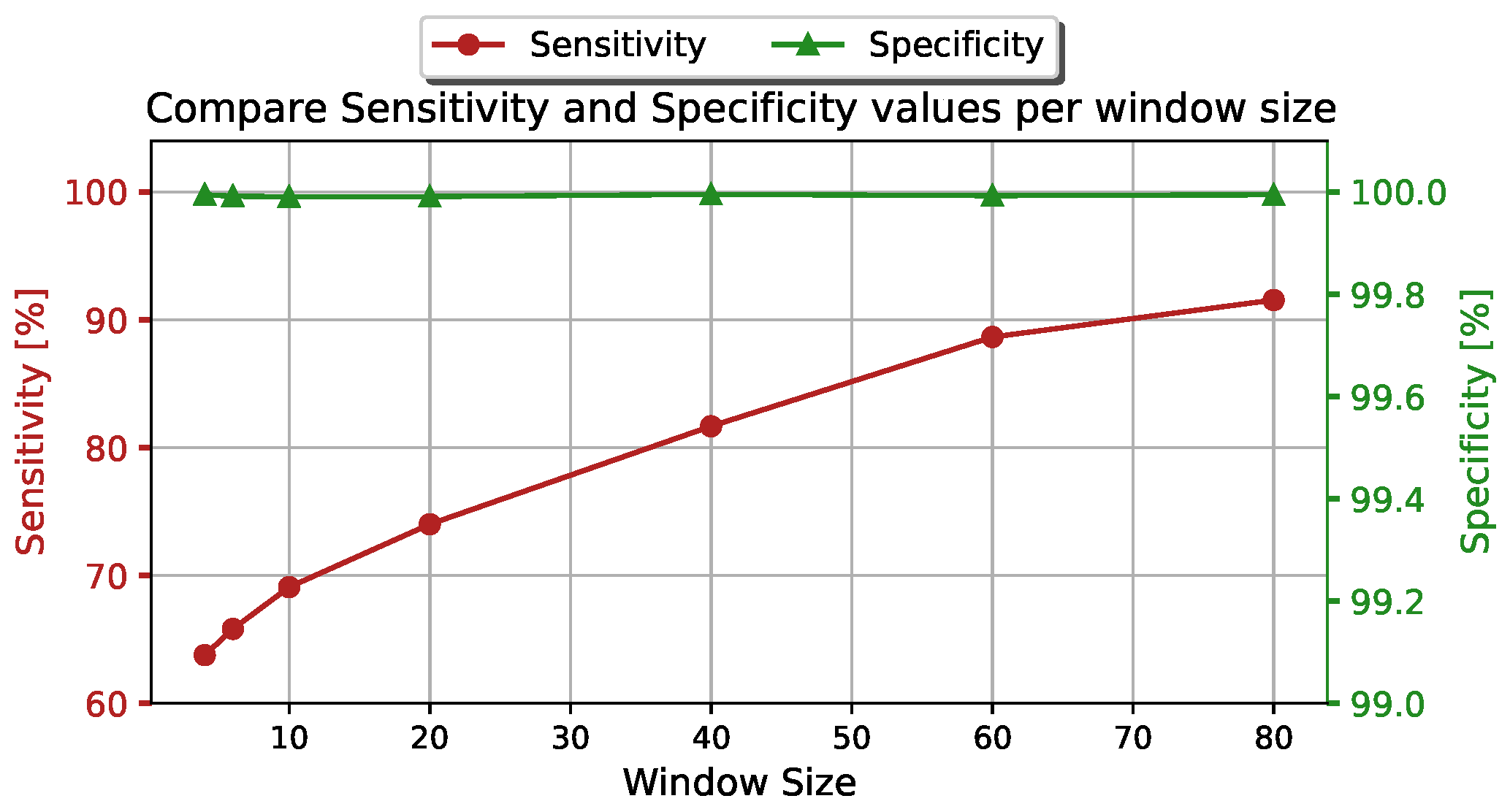
Figure 5 visualizes the sensitivity and specificity over the different inspected window sizes. The sensitivity addresses the fall and the specificity the climbing class. With an increasing window size, the sensitivity was the only one out of the two metrics that increased as well. We reached values of around when relying on a window size of 80 time steps (WS-80). This increased by almost compared to a window size of 4 (WS-4). In the best case, a total amount of 1941 samples out of all fall samples were falsely classified. The specificity, on the other hand, remained on a comparable level with an average value of around . Best results were achieved by relying on a window size of 40 (WS-40) with a metric value of around . This led to 66 false positives in total. However, this was the expected behavior, as we focused on reducing the false positives in the first place.
The HC-4 model detects falls with an accuracy of and climbing sequences with an accuracy of . Hence, we were reaching velocities above whilst handing out rope, and the threshold for the rope velocity whilst falling was reached in roughly a quarter of all time steps.
4.2. Analysis of False Positive Sequences
The duration of the fall of a climber depends on the height of the fall, the amount of slack in the system, the last clipped quickdraw and the reaction time of the belayer to stop the rope movement. It is usually a process which lasts for a couple of seconds. Our recordings show an average time of s ±s until a fall was identified. This leads to fall distances of around m ±m, which makes it necessary to catch a fall as fast as possible. However, it is also important to reduce the amount of false positive samples. In order to account for a realistic identification of false positive samples, we excluded consecutive false positive samples until the sequence is finished. Such a sequence would be:
- Handing out rope;
- Pulling rope back in;
- Moving without handing out rope.
If one sample within such a sequence included a false positive sample, the complete sequence was categorized as a false positive sequence. Overall, we registered 1924 such sequences, leading to an average of around 42 sequences per climbing ascent on average. By adjusting the class weights, the deep learning models were specifically designed to keep the amount of false positives at a relatively low level. Throughout all models, they range from 4 to 12, see Figure 6. The HC-4 model performed worst with a false positive rate of . Compared to that, the WS-40 model performed best by classifying four sequences falsely.
4.3. Fall Identification Time
This section further analyzes the fall sequences and their required time until it is identified as such. We will first analyze representative samples to address the problem and subsequently adapt the assumptions regarding a general statement.
4.3.1. Analysis of Pre-Selected Fall Sequences
The subgraphs in Figure 7 visualize specifically chosen fall sequences depicting best-case scenarios regarding the model prediction time. Especially two models were of interest and compared against the baseline model, the WS-6 and WS-20 models. Sub-graphs (a) and (b) visualize the comparison against the WS-6 and (c) and (d) against the WS-20 model. Our models were at least once outperformed by the baseline model. The largest temporal difference is shown in the sub-graphs (a) and (c) for the respective models. In both cases, the baseline model was faster in identifying the fall by less than ms reaching a comparable fall distance with a discrepancy of around cm.
On the other side, our models were able to outperform the baseline model by around ms, which leads to a reduced fall distance of around m. Those are visualized in the sub-graphs (b) and (d). In each case, our models performed best on the same fall, where the device was held in hand and neither slack nor fall potential were applied. Its velocity profile allows for an inference about friction in the system leading to a consistent velocity of the climber for a certain time period. Such a behavior can also be seen within sub-graph (a). However, the plateau is on a higher velocity level. The investigation of such a plateau is an important aspect as its duration and level can cause a climber to fall onto the ground when relying solely on the threshold approach.
4.3.2. Configuration-Wise Analysis of the Prediction Time
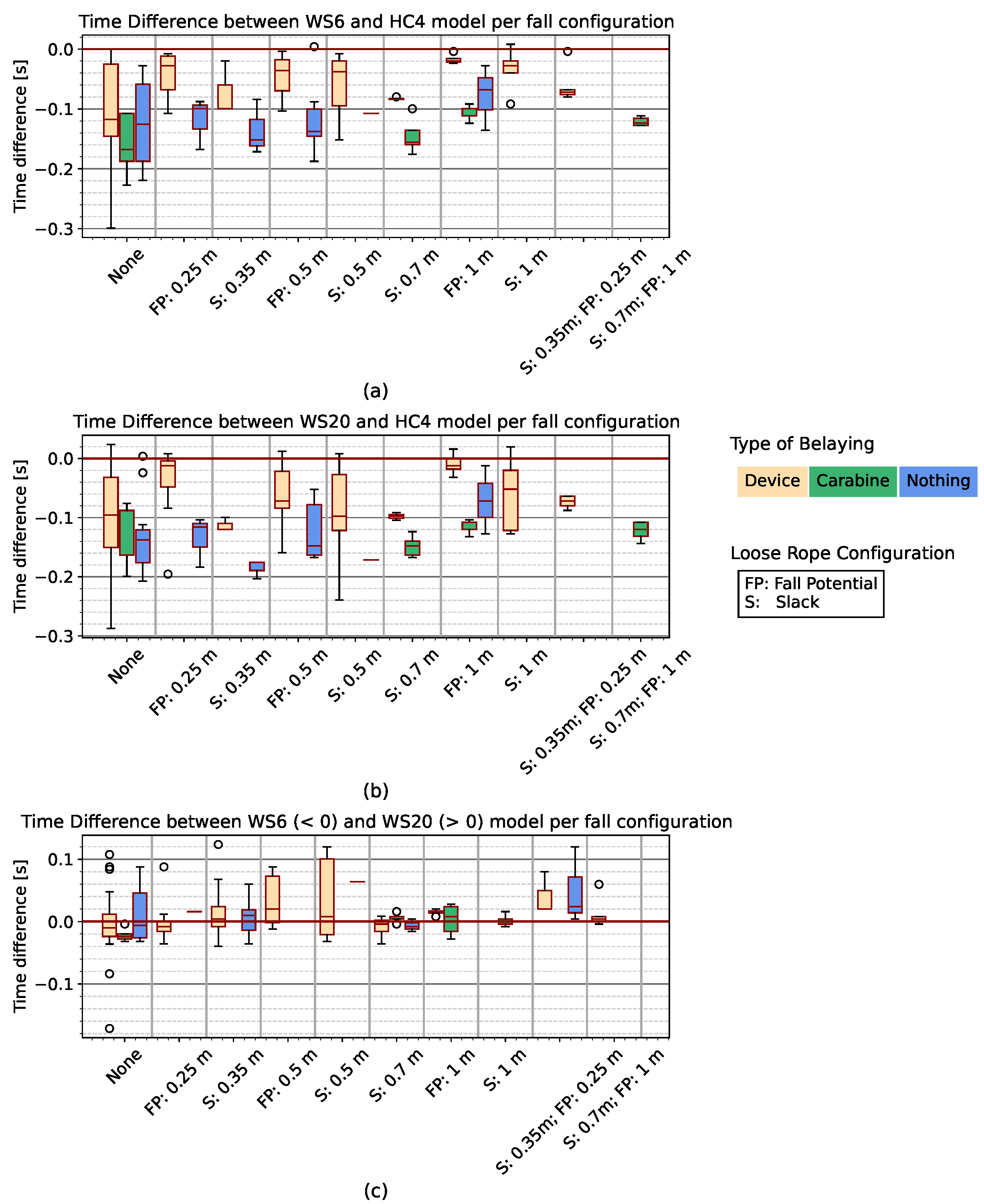
Each of the configurations described in Section 3.2 influence the movement behaviour of the belay device. So, it is a valid assumption that they also have an impact on the required time to identify a fall. The results in this regard are shown in Figure 8. Its sub-graphs (a) and (b) visualize the time difference between the predictive models and the baseline model. Compared to those graphs is sub-graph (c), which visualizes the time difference between the two predictive models, WS-6 and WS-20. Both predictive models outperformed the baseline model by at least of the recorded falls per configuration.
- Comparison between the WS-6 and baseline model
In only two cases was the WS-6 model slower in predicting a fall than the threshold approach, see Figure 8a. One of these was while having a fall potential of m and not holding the device in hand, and once while holding the device with an additional amount of slack of m in the system. Interestingly, the impact of doubling the fall potential from m to m only slightly decreased the time difference between the two models, hence benefiting the WS-6 model. By increasing the fall potential further to m, the time difference came closer to s. This moves closer along with the observation of a steeper velocity curve, which leads to the threshold value being reached earlier.
Another analysis regarding the slack parameter resulted in negligible time differences regarding the median level, even though it was doubled from m to m.
- Comparison between the WS-20 and baseline model
The WS-20 model includes 20 time steps per sample. This leads to the certitude that a fall had to be at least s progressed until the model was able to identify it as such. This is around the same amount of time as the median time difference between the WS-20 and the baseline model for the configuration of no slack or fall potential whilst holding the device in hand, compared in Figure 8b. The same configuration also includes the highest and lowest time differences with s and s. In general, a positive time benefits the baseline model, whereas a negative time represents a faster fall prediction using the WS-20 model. Overall, 13 fall sequences were identified faster by relying on the threshold approach. Most of them can be assigned to the configuration whilst holding the device in hand. In only one case was the carabiner held. Loose rope is an additional factor, where 9 out of those 13 sequences had slack or fall potential. In those cases, the climbers initial velocity when he is starting to fall into the rope increases with the amount of loose rope. This is supposed to benefit the threshold approach. Though, the additional registered falling height compared to the WS-20 model was less than cm.
- Comparison between the WS-6 and WS-20 model
The window size is an important factor when it comes to time series analysis. A single sample can be decisive about the outcome, especially in such a fast environment like sports climbing. Therefore, this subsection provides an analysis between a 6 sample size window and a window containing 20 samples. The summary of the time differences is visualized in Figure 8c.
In of the fall sequences, the WS-6 model was faster than the WS-20 model. Holding the belay device in hands and either having no slack or fall potential at all or the fall was conducted with fall potential solely favored the WS-6 model. This way, more than half of those sequences were predicted faster with the WS-6 model. It was able to detect a fall up to ms faster. Compared to that, having slack in the system favored the prediction time of the WS-20 model. In of those fall sequences, the WS-20 model was faster in detecting the respective falls. However, none of the sequences with slack were as fast as one sequence from the configuration of having half a meter of fall potential. It predicted the fall ms faster using the WS-20 over the WS-6 model. However, interestingly, the WS-6 model required at least 21 samples to predict a fall, leading to the assumption that the progression of the fall itself is decisive for the prediction.
4.3.3. Window Size Dependant Prediction Time and Comparison with the Baseline Model
The window size has a direct influence regarding the possible prediction time. On the one side, a larger window size is able to store more information about the fall itself, thought, it also increases the shortest possible prediction time. So far, two specific window sizes containing either 6 or 20 samples were analyzed. This section provides a broader overview over the investigated window sizes with an increased spectrum regarding their size. We analyzed windows with 4, 6, 10, 20, 40, 60 and 80 samples.
- Prediction time per window size
The size of the time window is decisive about the required time for predicting a fall. The blue dotted line in Figure 9a represents the minimal possible time to identify a fall for the respective time window. The largest three window sizes were able to recognize a fall within their first window of the sequence. Reducing the size only increased the discrepancy between what is possible and the true identification time, except for the WS-4 model. In the best case, it was able to be slightly faster than the WS-10 model. The fastest possible identification times were achieved using the models WS-4 and WS-20 with ms and ms, respectively.
- Time difference between prediction time and HC-4 model
Figure 9a visualizes the absolute times when the prediction of a fall occurred. It is not possible to draw a conclusion about the effectiveness of the predictive models compared to the threshold approach. Hence, we analyzed the time difference between them, which is visualized in Figure 9b. Positive values benefit the HC-4 model whereas negative values are in favor of the predictive models. The fastest time difference was achieved with the WS-6 model with a difference of around ms. In contrast, the WS-80 model contains the largest positive outlier with a value above ms. It is also the only model where more than of the sequences were detected faster by the comparison model.
Based on the median metric, the performance improved by increasing the window size until reaching a size of 20. From there on, it started to decrease again. This correlates with the findings from Figure 9a, where the minimum possible time overlaps with the fastest prediction time.
4.4. Summary of the Results
This section provides a summary of the results by comparing the models regarding the most important metrics. The false positive rate describes the rate with which the model predicts a sequence of handing out rope as a fall. The lowest rate provided the WS-40 model with a rate of about . The fall identification time represents the moment until the respective model predicts a fall correctly. Whereas the WS-20 model was fastest in predicting a fall correctly on average, the WS-80 model performed worst with comparable times as the reference model. This summary is highlighted in Table 2.
5. Discussion
In this paper, we address the issue of time windows in a time critical environment. The approach is applied onto the domain of sport climbing, more specifically, the identification of the fall of a climber. A normed fall is defined by a fall height of m, which leads to a fall time of less than a second. The decision for the time windows’ length is therefore a critical parameter as the amount of included time steps has a direct influence on the time to identify the task. We show that a larger time window is able to classify more samples correctly. The largest window size is able to outscore the comparison model’s sensitivity value by over . However, metrics like sensitivity and specificity are only part of the evaluation for the underlying task. In a time-critical environment, the time of identification is more important than the overall accuracy of the model. Our analysis of the different time window lengths shows that larger time windows have the disadvantage of late identification. A window with 80 samples requires at least s to identify a fall which results in an additional fall height of m. It highlights the necessity for a critical analysis of the problem itself.
High accuracy or sensitivity and specificity are mainly a good indicator towards a well-trained and generalized neural network model. However, in reality, this is not necessarily true. Our investigations show the dependency of the window size compared to the performance scores. With an increasing window size, the sensitivity increased as well, but the performance of the model with respect to the identification time of the fall decreased. So, depending on the initial research question, the performance indicator might change. In our case, the combination of correctness and timing was the decisive factor.
The most difficult sequences from the class Fall belong to the configuration of holding the device in hand without any initial slack and fall potential. They resemble sequences of handing out rope the most. However, our configurations resemble only a fraction from all possibilities. We neglected top rope situations as well as overhang sections, as setting up the measurement system in a sport climbing environment where a sandbag serves as a human substitute is time- and money-consuming. Especially, falling whilst top rope climbing has the potential to lead to comparable sequences as handing out rope. Further studies have to be conducted in order to address this topic and re-evaluate the models.
The same is applicable to the climb scenarios. Overhang sections are missing as well as routes with varying difficulty and climber with different experience. The climbing routes are oriented in the fifth grade of the UIAA scale.
The amount of samples to train, validate and test the neural network models was over one million. Even the minority class contains almost 50,000 samples. However, we only recorded 161 fall and 48 climb sequences in total. As only the time of identification is relevant for the fall sequences, it decreases the information gain and variance within the sample space. So, recording more falls and ascents would have a positive effect on the model’s performance.
Before using such a system as a backup safety device in the area of sport climbing, the amount of false positives has to further decrease. In this study, we separated the climbing sequences in two classes. The class Waiting contains highly resembling sequences with almost no information about a climbing activity. The initial idea behind keeping those sequences was to analyze any potential information gain shortly before the fall occurred, especially for window sizes with less than ms. Though, we found out, that a certain amount of activity is required to identify a fall. By reducing the data set this way, we finally have 1924 sequences of handing out rope and 161 falls. In addition to the imbalance between those two classes, fall sequences without any fall potential and slack remain most difficult to be distinguished from the other class. Synthesizing those sequences could enhance the variability within the specific configuration and improve the results.
6. Conclusions and Outlook
In this paper we applied deep learning models to identify a climber’s fall based on the information from a multi-sensor system attached to a belay device. A previous study by Oppel et al. [15] could demonstrate that the system is able to register rope movement as well as the movement of the belay device itself and shows the possibility of classifying a fall with it. However, the time of identification was neglected in the previous work. As such a system can serve as a back-up safety system, this is a critical factor.
Our time window analysis shows the necessity for a critical evaluation of the model parameter—in our case, the time window. Depending on the amount of included time steps, the model performed better or worse than the comparison model, which relies on the rope velocity to identify a fall. The best results in the sense of the accuracy of the model were achieved with the highest window size possible. The sensitivity increased from around to . However, the time of identification dropped in the best case from ms with the WS-80 model to ms with the WS-4 model.
Our analysis shows that our deep learning models outperform the threshold approach in the detection of false positive samples, independent of the window size. In the best case, the deep learning model with a window size of 40 time steps lead to a false positive rate of . This would statistically lead to a falsely classified sequence of handing out rope once in every 416 registrations, or once every 9th route.
Our study shows the possibility of using such a system as a back-up safety system. Though, the climbing data was recorded on a single wall with a height of m and 4 different belayer around the same skill level. It would be beneficial to further investigate the system in a broader study with belayers of varying skill levels in order validate the results for a broader spectrum of climbers/belayers. Additionally, different types of wall structures like an overhang section or the fall of a real climber might influence the predictive behavior of the algorithm.
Our time window analysis showed promising results in using an instrumented belay device for monitoring the fall of a climber in real time. As it is not only capable of extracting information about the climber, but also about the belayer, it would be interesting to utilize the device for teaching purposes; especially, the type of belaying in a fall situation and the way of handing out rope could be analyzed. As a previous study by Oppel et al. [17] showed that the type of belaying has a direct influence on the severity of a fall. Handing out rope can be a time-critical activity as well. By not handing out rope fast enough, the climber starts to wear out faster. So, it would be interesting to see if the device is capable of monitoring those activities to improve the safety and skill level of climber and belayer.
Author Contributions
Conceptualization, M.M.; Data curation, H.O.; Formal analysis, H.O. and M.M.; Funding acquisition, M.M.; Investigation, H.O. and M.M.; Methodology, H.O. and M.M.; Project administration, M.M.; Resources, M.M.; Software, H.O. and M.M.; Supervision, M.M.; Validation, H.O. and M.M.; Visualization, H.O.; Writing—original draft, H.O.; Writing—review and editing, M.M. All authors have read and agreed to the published version of the manuscript.
Funding
This project was funded by the Federal Ministry for Economic Affairs and Climate Action (BMWK) and their Central Innovation Programme (ZIM) for small and medium-sized enterprises (SMEs).
Institutional Review Board Statement
Not applicable.
Informed Consent Statement
Not applicable.
Data Availability Statement
The data presented in this study are available on request from the corresponding author. The data are not publicly available due to the project partner from the ZIM project is the co-owner of the data.
Acknowledgments
We acknowledge the Edelrid GmbH & Co. KG for their support and contribution throughout this research project.
Conflicts of Interest
The authors declare that the monitoring system in this study is directly integrated into a belay device from the Edelrid GmbH & Co. KG (Achener Weg 66, 88316 Isny im Allgäu) company. The company was only involved in the data collection, but was not involved in the study design, analysis, interpretation of data, the writing of this article, or the decision to submit it for publication.
References
- Castro, R.; Mujica, G.; Portilla, J. Internet of Things in Sport Training: Application of a Rowing Propulsion Monitoring System. IEEE Internet Things J. 2022, 19, 18880–18897. [Google Scholar] [CrossRef]
- Ren, J.; Guan, F.; Pang, M.; Li, S. Monitoring of human body running training with wireless sensor based wearable devices. Comput. Commun. 2020, 157, 343–350. [Google Scholar] [CrossRef]
- Munz, M.; Engleder, T. Intelligent Assistant System for the Automatic Assessment of Fall Processes in Sports Climbing for Injury Prevention based on Inertial Sensor Data. Curr. Dir. Biomed. Eng. 2019, 5, 183–186. [Google Scholar] [CrossRef]
- Kim, J.; Chung, D.; Ko, I. A climbing motion recognition method using anatomical information for screen climbing games. Hum. Centric Comput. Inf. Sci. 2017, 7, 25. [Google Scholar] [CrossRef]
- Bonfitto, A.; Tonoli, A.; Feraco, S.; Zenerino, E.C.; Galluzzi, R. Pattern recognition neural classifier for fall detection in rock climbing. Proc. Inst. Mech. Eng. Part P J. Sport. Eng. Technol. 2019, 233, 478–488. [Google Scholar] [CrossRef]
- Baláš, J.; Panáčková, M.; Strejcová, B.; Martin, A.J.; Cochrane, D.J.; Kaláb, M.; Kodejška, J.; Draper, N. The relationship between climbing ability and physiological responses to rock climbing. Sci. World J. 2014, 2014, 678387. [Google Scholar] [CrossRef] [PubMed]
- Breen, M.; Reed, T.; Breen, H.M.; Osborne, C.T.; Breen, M.S. Integrating Wearable Sensors and Video to Determine Microlocation-Specific Physiologic and Motion Biometrics-Method Development for Competitive Climbing. Sensors 2022, 22, 6271. [Google Scholar] [CrossRef] [PubMed]
- Hacques, G.; Dicks, M.; Komar, J.; Seifert, L. Visual control during climbing: Variability in practice fosters a proactive gaze pattern. PLoS ONE 2022, 17, e0269794. [Google Scholar] [CrossRef] [PubMed]
- Watts, P.; Jensen, R.; Gannon, E.; Kobeinia, R.; Maynard, J.; Sansom, J. Forearm EMG During Rock Climbing Differs from EMG During Handgrip Dynamometry. Int. J. Exerc. Sci. 2008, 1, 2. [Google Scholar]
- Baláš, J.; Gajdošík, J.; Giles, D.; Fryer, S.; Krupková, D.; Brtník, T.; Feldmann, A. Isolated finger flexor vs. exhaustive whole-body climbing tests? How to assess endurance in sport climbers? Eur. J. Appl. Physiol. 2021, 121, 1337–1348. [Google Scholar] [CrossRef] [PubMed]
- Boulanger, J.; Seifert, L.; Hérault, R.; Coeurjolly, J.-F. Automatic Sensor-Based Detection and Classification of Climbing Activities. IEEE Sensors J. 2016, 16, 742–749. [Google Scholar] [CrossRef]
- Seifert, L.; Cordier, R.; Orth, D.; Courtine, Y.; Croft, J.L. Role of route previewing strategies on climbing fluency and exploratory movements. PLoS ONE 2017, 12, e0176306. [Google Scholar] [CrossRef] [PubMed]
- Ladha, C.; Hammerla, N.Y.; Olivier, P.; Plötz, T. ClimbAX: Skill Assessment for Climbing Enthusiasts. In UbiComp 2013: Proceedings of the 2013 ACM International Joint Conference on Pervasive and Ubiquitous Computing, Zurich, Switzerland, 8–12 September 2013; ACM: New York, NY, USA, 2013. [Google Scholar] [CrossRef]
- Seifert, L.; Dovgalecs, V.; Boulanger, J.; Orth, D.; Hérault, R.; Davids, K. Full-body movement pattern recognition in climbing. Sport. Technol. 2014, 7, 166–173. [Google Scholar] [CrossRef]
- Oppel, H.; Munz, M. Intelligent Instrumented Belaying System in Sports Climbing. In Sensors and Measuring Systems, Proceedings of the 21th ITG/GMA-Symposium, Nuremberg, Germany, 10–11 May 2022; VDE: Frankfurt am Main, Germany, 2022; pp. 1–7. [Google Scholar]
- Madgwick, S.O.H.; Harrison, A.J.L.; Vaidyanathan, R. Estimation of IMU and MARG orientation using a gradient descent algorithm. In Proceedings of the 2011 IEEE International Conference on Rehabilitation Robotics, Zurich, Switzerland, 21 June–1 July 2011; pp. 1–7. [Google Scholar] [CrossRef]
- Oppel, H.; Munz, M. Analysis of Feature Dimension Reduction Techniques Applied on the Prediction of Impact Force in Sports Climbing Based on IMU Data. AI 2021, 2, 662–683. [Google Scholar] [CrossRef]
Figure 1.
Example of a climbing fall with a fall potential of m. Start (violet) and end point (turquoise) of the fall sequence are equivalent to the time stamp of the impact force. The initial time stamp of the cut sequence for the neural network models (pink), the endpoint of the free fall prior to falling into the rope (black), the beginning of the fall into the rope (orange) as well as the progression of the resulting accelerations of the climber (red) and belayer (blue) and the cumulative rope distance (green) over time.

Figure 2.
Sequence from a climb scenario. The graph depicts three different areas. The white area represents the sequence, where no rope movement was registered and the resulting acceleration of the belay device is below , the orange area displays a sequence where the belay device registered resulting accelerations above and the red area highlights rope movement sequences.

Figure 3.
Influence of the window size on the total amount of samples per class (left graph) and the class fractions (right graph).
Figure 3.
Influence of the window size on the total amount of samples per class (left graph) and the class fractions (right graph).

Figure 4.
The CNN architecture for handling the automatic feature engineering and classification task.
Figure 4.
The CNN architecture for handling the automatic feature engineering and classification task.

Figure 5.
Sensitivity (red) and specificity (green) are plotted over the different window sizes. With increasing window size the sensitivity increase as well. The specificity is remaining on an equivalent level over all window sizes.
Figure 5.
Sensitivity (red) and specificity (green) are plotted over the different window sizes. With increasing window size the sensitivity increase as well. The specificity is remaining on an equivalent level over all window sizes.

Figure 6.
Probability of an occurring false positive sequence whilst handing out rope, which is defined as a consecutive sequence of registered rope velocity over at least s. Overall, 1924 sequences of handing out rope were registered throughout all recorded climb scenarios. Most false positive sequences occurred with the HC-4 model, whereas the best results were achieved with the deep learning model having a window size of 40 time steps. It registered three times fewer false positives, i.e., the amount of falsely identified rope pulls classed as a climbing fall.
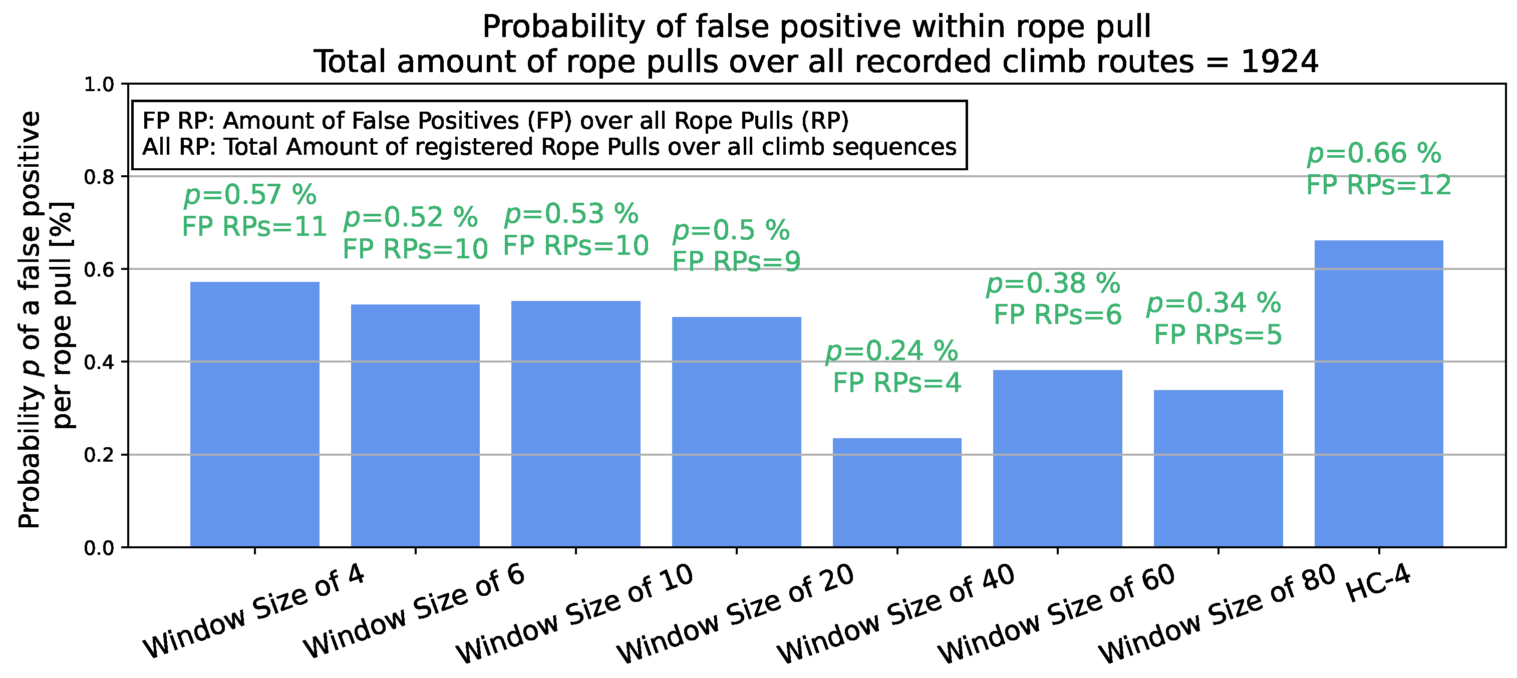
Figure 7.
Visualization of fall scenarios to analyze the identification times with the respective models. Worst- (a) and best- (b) case scenarios between the WS-6 and HC-4 model are compared. The same visual comparison is conducted for the WS-20 with the HC-4 model in the worst (c) and best (d) case. Both predictive models outscore the HC-4 model regarding the most beneficial prediction time. They were at least 15 times faster than their counterpart sequence from the HC-4 model.

Figure 8.
Time differences between the predictive model using a window size of 6 (a) and 20 samples (b) and the HC-4 model. The distributions are visualized separately for each configuration. A time value below zero indicates that the predictive model is faster in the identification of a fall, whereas a time value above zero indicates that the HC-4 model is faster. The blue boxes reference the configuration without any fall potential or slack in the system. The yellow boxplots identify fall situations where the belayer was holding the belay device in hand, whereas the green boxplots visualize the configuration of the belayer holding the carabine throughout a fall. Additionally, the two predictive models were compared in the subgraph (c) in the same way the two models were compared to the reference model.

Figure 9.
Distribution of times until a fall is identified as such (a) and sequence comparison of moments until fall identification between the deep learning models and the HC-4 model (b). The orange lines represent the median.
Figure 9.
Distribution of times until a fall is identified as such (a) and sequence comparison of moments until fall identification between the deep learning models and the HC-4 model (b). The orange lines represent the median.


Table 1.
Setup of the recorded fall configurations. Variations in fall potential and slack were chosen to depict the reality as close as possible [15].
Table 1.
Setup of the recorded fall configurations. Variations in fall potential and slack were chosen to depict the reality as close as possible [15].
| Setup Number | Belay Device Handling | Number of Recordings | Slack [m] | Fall Potential [m] |
|---|---|---|---|---|
| 1 | Device | 42 | 0.00 | 0.00 |
| 2 | Device | 3 | 0.35 | 0.00 |
| 3 | Device | 10 | 0.50 | 0.00 |
| 4 | Device | 4 | 0.70 | 0.00 |
| 5 | Device | 10 | 1.00 | 0.00 |
| 6 | Device | 13 | 0.00 | 0.25 |
| 7 | Device | 19 | 0.00 | 0.50 |
| 8 | Device | 7 | 0.00 | 1.00 |
| 9 | Device | 5 | 0.35 | 0.25 |
| 10 | Carabiner | 5 | 0.00 | 0.00 |
| 11 | Carabiner | 5 | 0.70 | 0.00 |
| 12 | Carabiner | 5 | 0.00 | 1.00 |
| 13 | Carabiner | 5 | 0.70 | 1.00 |
| 14 | Nothing | 12 | 0.00 | 0.00 |
| 15 | Nothing | 3 | 0.35 | 0.00 |
| 16 | Nothing | 1 | 0.50 | 0.00 |
| 17 | Nothing | 3 | 0.00 | 0.25 |
| 18 | Nothing | 6 | 0.00 | 0.50 |
| 19 | Nothing | 3 | 0.00 | 1.00 |
Table 2.
Summary of the results comparing the model against each other.
| WS 4 | WS 6 | WS 10 | WS 20 | WS 40 | WS 60 | WS 80 | HC-4 | |
|---|---|---|---|---|---|---|---|---|
| FP-rate [%] | 0.57 | 0.52 | 0.53 | 0.50 | 0.24 | 0.38 | 0.34 | 0.66 |
| Fall identification time [ms] |
Disclaimer/Publisher’s Note: The statements, opinions and data contained in all publications are solely those of the individual author(s) and contributor(s) and not of MDPI and/or the editor(s). MDPI and/or the editor(s) disclaim responsibility for any injury to people or property resulting from any ideas, methods, instructions or products referred to in the content. |
© 2023 by the authors. Licensee MDPI, Basel, Switzerland. This article is an open access article distributed under the terms and conditions of the Creative Commons Attribution (CC BY) license (https://creativecommons.org/licenses/by/4.0/).
Share and Cite
MDPI and ACS Style
Oppel, H.; Munz, M. A Time Window Analysis for Time-Critical Decision Systems with Applications on Sports Climbing. AI 2024, 5, 1-16. https://doi.org/10.3390/ai5010001
AMA Style
Oppel H, Munz M. A Time Window Analysis for Time-Critical Decision Systems with Applications on Sports Climbing. AI. 2024; 5(1):1-16. https://doi.org/10.3390/ai5010001
Chicago/Turabian StyleOppel, Heiko, and Michael Munz. 2024. "A Time Window Analysis for Time-Critical Decision Systems with Applications on Sports Climbing" AI 5, no. 1: 1-16. https://doi.org/10.3390/ai5010001