

Single Image Super Resolution Using Deep Residual Learning


Abstract
1. Introduction
2. Related Work
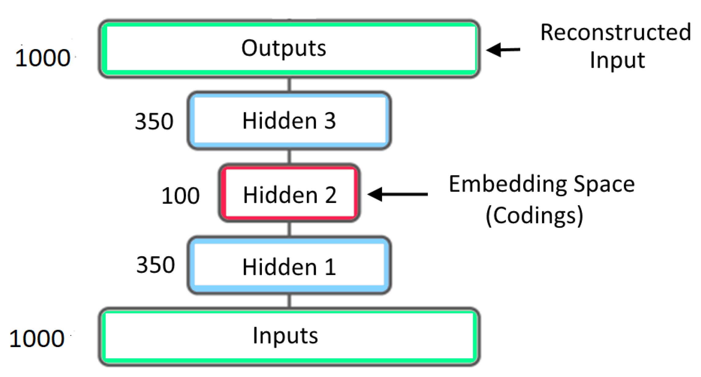
3. Autoencorders
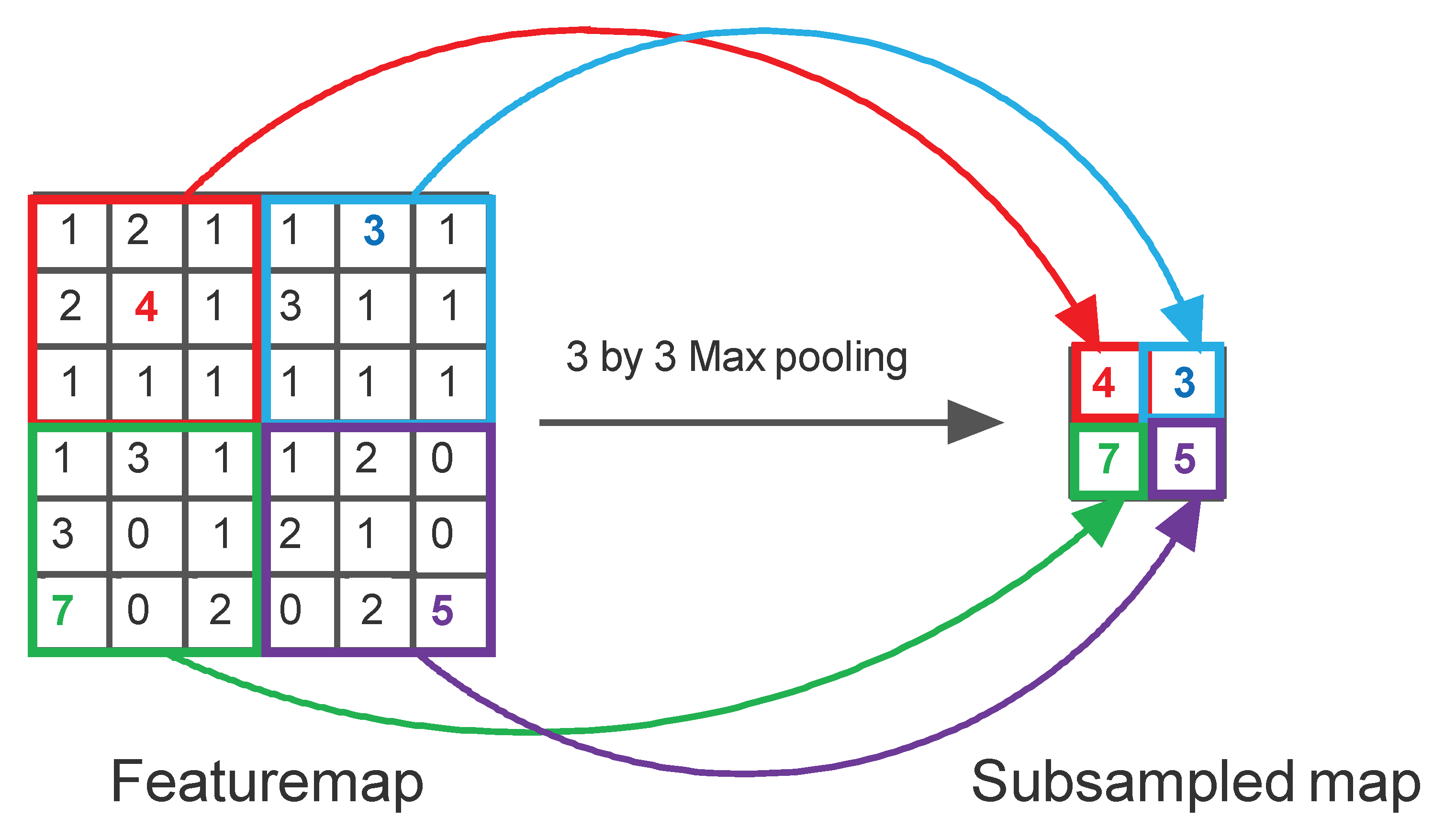
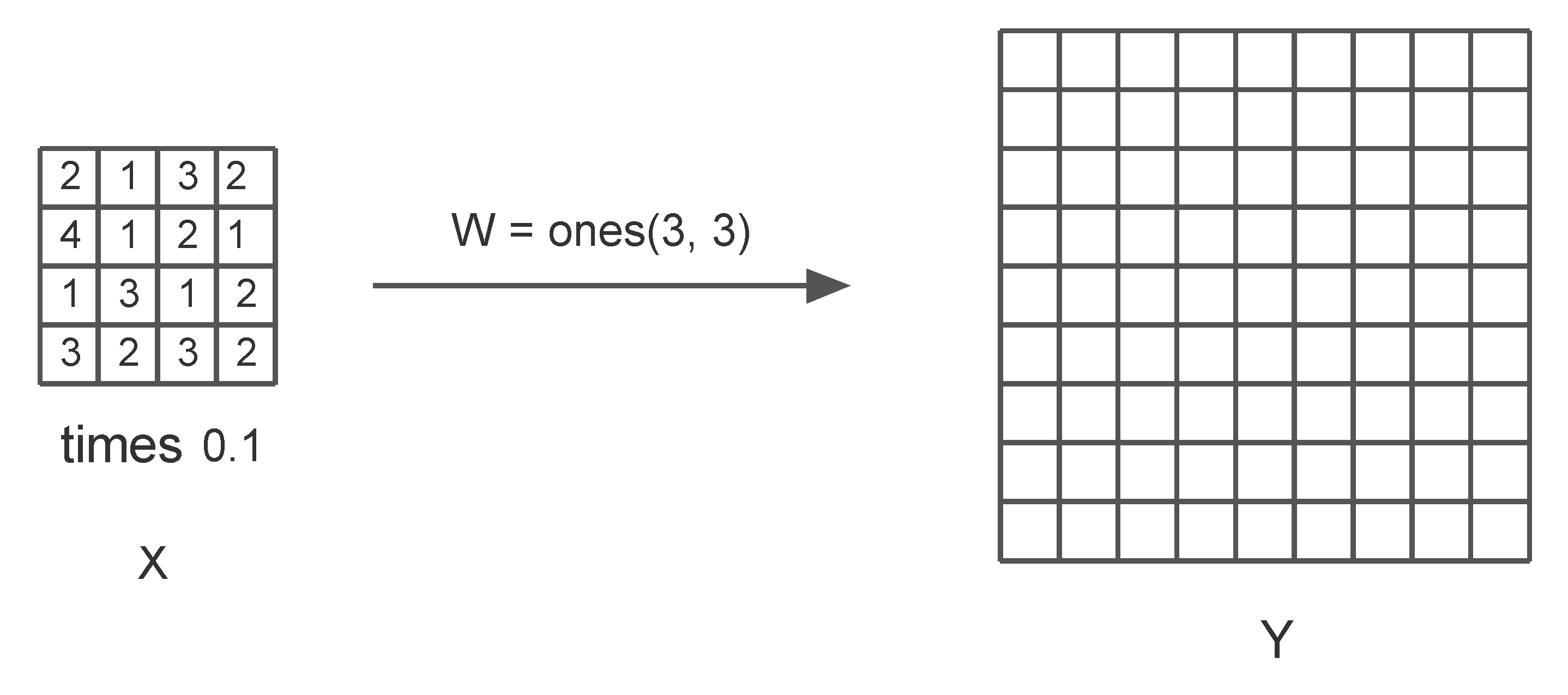
4. Problem Statement and the Model
5. Proposed Method
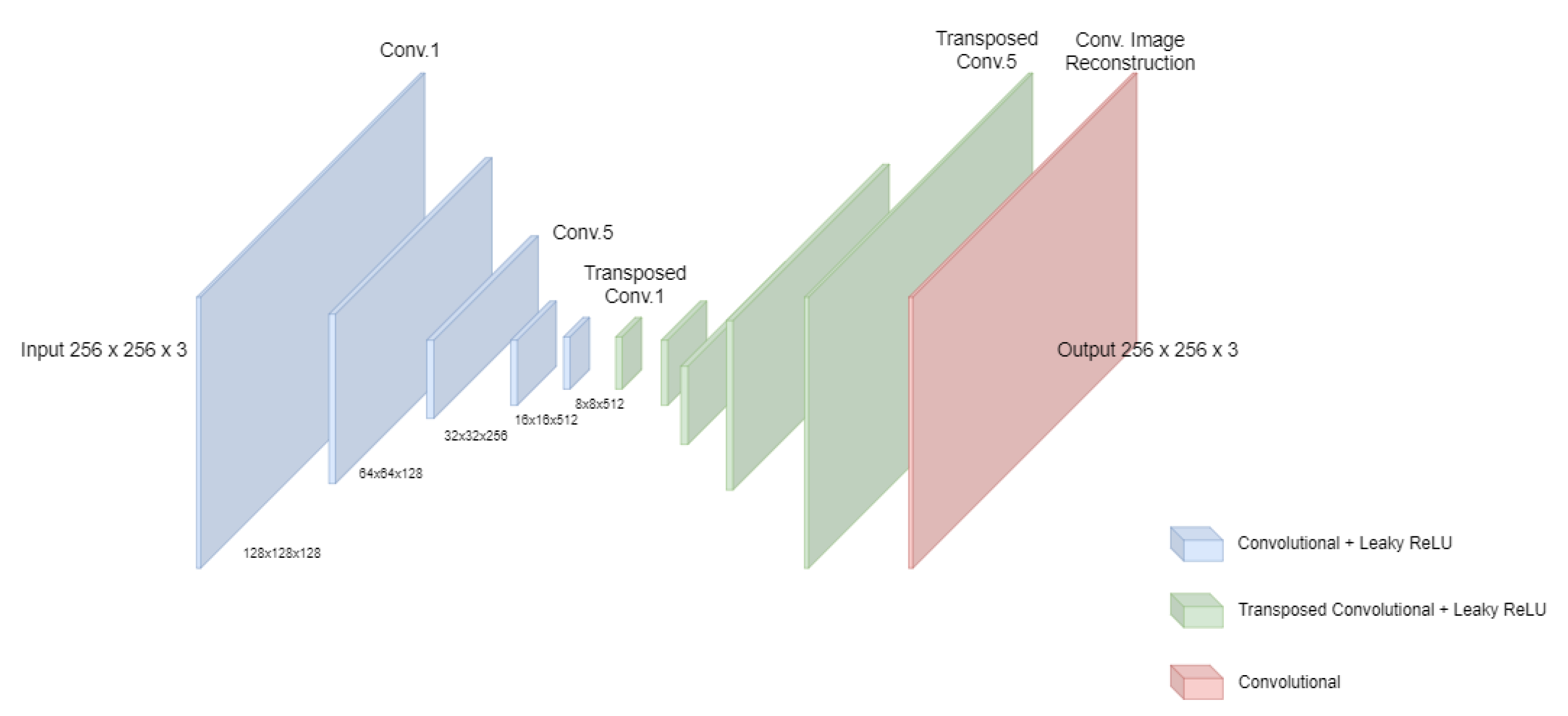
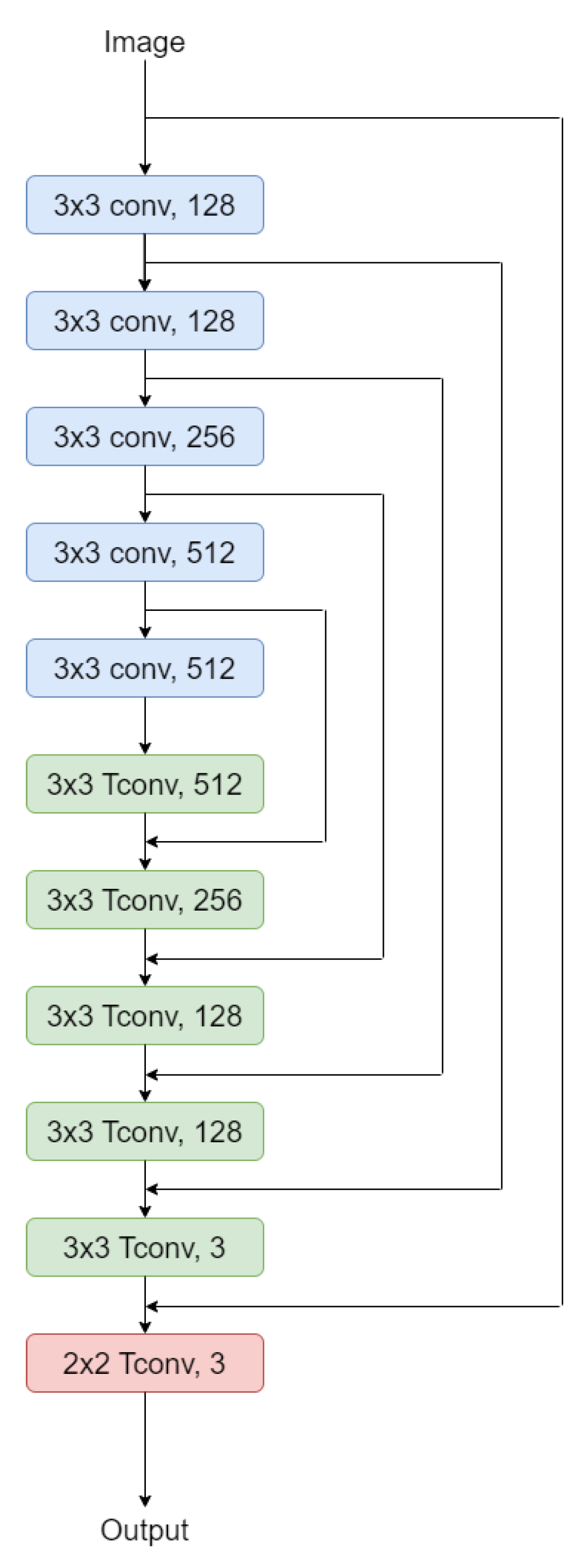
5.1. Proposed Network
5.2. Training
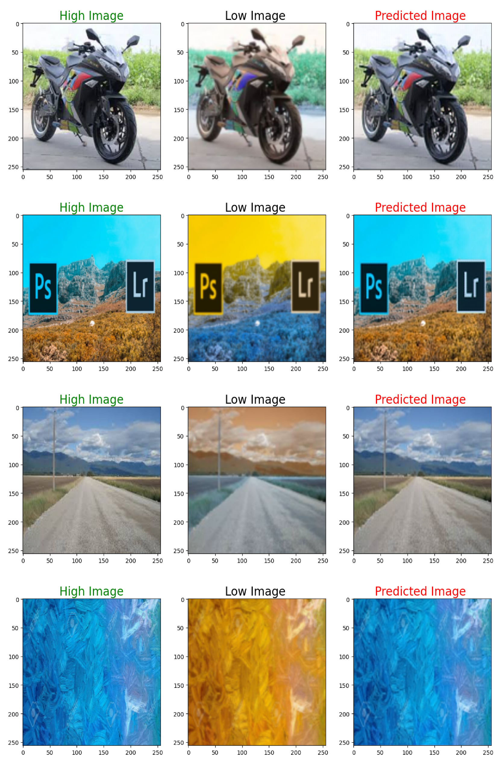
6. Experiments and Results
6.1. Training Data
6.2. Training Parameters
6.3. Model and Performance Trade-Off
7. Conclusions
Author Contributions
Funding
Institutional Review Board Statement
Informed Consent Statement
Data Availability Statement
Conflicts of Interest
Appendix A
References
- Keys, R. Cubic convolution interpolation for digital image processing. IEEE Trans. Acoust. Speech Signal Process. 1981, 29, 1153–1160. [Google Scholar] [CrossRef]
- Duchon, C.E. Lanczos filtering in one and two dimensions. J. Appl. Meteorol. 1979, 18, 1016–1022. [Google Scholar] [CrossRef]
- Dai, S.; Han, M.; Xu, W.; Wu, Y.; Gong, Y.; Katsaggelos, A.K. Softcuts: A soft edge smoothness prior for color image super-resolution. IEEE Trans. Image Process. 2009, 18, 969–981. [Google Scholar] [PubMed]
- Sun, J.; Xu, Z.; Shum, H.Y. Image super-resolution using gradient profile prior. In Proceedings of the IEEE Conference on Computer Vision and Pattern Recognition, Anchorage, AK, USA, 23–28 June 2008; pp. 1–8. [Google Scholar]
- Yan, Q.; Xu, Y.; Yang, X.; Nguyen, T.Q. Single image super-resolution based on gradient profile sharpness. IEEE Trans. Image Process. 2015, 24, 3187–3202. [Google Scholar] [PubMed]
- Marquina, A.; Osher, S.J. Image super-resolution by TV-regularization and Bregman iteration. J. Sci. Comput. 2008, 37, 367–382. [Google Scholar] [CrossRef]
- Krizhevsky, A.; Sutskever, I.; Hinton, G.E. ImageNet Classification with Deep Convolutional Neural Networks. Commun. ACM 2017, 60, 84–90. [Google Scholar] [CrossRef]
- Hinton, G.E.; Zimel, R.S. Autoencoders, Minimum Description Length and Helmholtz Free Energy. In Proceedings of the Advances in Neural Information Processing Systems 6 (NIPS 1993), Denver, CO, USA, 29 November–2 December 1993; pp. 600–605. [Google Scholar]
- Dong, C.; Loy, C.C.; He, K.; Tang, X. Image super-resolution using deep convolutional networks. IEEE Trans. Pattern Anal. Mach. Intell. 2015, 38, 295–307. [Google Scholar] [CrossRef]
- Johnson, J.; Alahi, A.; Fei-Fei, L. Perceptual losses for real-time style transfer and super-resolution. In Proceedings of the European Conference on Computer Vision, Amsterdam, The Netherlands, 11–14 October 2016; pp. 694–711. [Google Scholar]
- Wang, Z.; Bovik, A.C. Mean squared error: Love it or leave it? a new look at signal fidelity measures. IEEE Signal Process. Mag. 2009, 26, 98–117. [Google Scholar] [CrossRef]
- Kundu, D.; Evans, B.L. Full-reference visual quality assessment for synthetic images: A subjective study. In Proceedings of the 2015 IEEE International Conference on Image Processing (ICIP), Quebec City, QC, Canada, 27–30 September 2015; pp. 3046–3050. [Google Scholar]
- Kim, J.; Lee, J.K.; Lee, K.M. Accurate Image Super-Resolution Using Very Deep Convolutional Networks. In Proceedings of the IEEE Conference on Computer Vision and Pattern Recognition, Las Vegas, NV, USA, 7–30 June 2016; pp. 1646–1654. [Google Scholar]
- He, K.; Zhang, X.; Ren, S.; Sun, J. Deep Residual Learning for Image Recognition. In Proceedings of the IEEE Conference on Computer Vision and Pattern Recognition, Las Vegas, NV, USA, 27–30 June 2016; pp. 770–778. [Google Scholar]
- Ledig, C.; Theis, L.; Huszár, F.; Caballero, J.; Cunningham, A.; Acosta, A.; Aitken, A.; Tejani, A.; Totz, J.; Wang, Z.; et al. Photo-realistic single image super-resolution using a generative adversarial network. In Proceedings of the IEEE Conference on Computer Vision and Pattern Recognition, Honolulu, HI, USA, 21–26 July 2017; pp. 105–114. [Google Scholar]
- Lim, B.; Son, S.; Kim, H.; Nah, S.; Lee, K.M. Enhanced deep residual networks for single image super-resolution. In Proceedings of the IEEE Conference on Computer Vision and Pattern Recognition Workshops, Honolulu, HI, USA, 21–26 July 2017; pp. 136–144. [Google Scholar]
- Zhang, Y.; Li, K.; Li, K.; Wang, L.; Zhong, B.; Fu, Y. Residual dense network for image super-resolution. In Proceedings of the IEEE Conference on Computer Vision and Pattern Recognition Workshops, Salt Lake City, UT, USA, 18–23 June 2018; pp. 39–48. [Google Scholar]
- Zhang, Y.; Tian, Y.; Kong, Y.; Zhong, B.; Fu, Y. Image super-resolution using very deep residual channel attention networks. In Proceedings of the European Conference on Computer Vision, Munich, Germany, 8 September 2018; pp. 286–301. [Google Scholar]
- Yang, W.; Zhang, X.; Tian, Y.; Wang, W.; Xue, J.H.; Liao, Q. Deep Learning for Single Image Super-Resolution: A Brief Review. IEEE Signal Process. Mag. 2019, 36, 110–117. [Google Scholar] [CrossRef]
- Gao, X. Pixel Attention Activation Function for Single Image Super-Resolution. In Proceedings of the IEEE International Conference on Consumer Electronics and Computer Engineering, Guangzhou, China, 6–8 January 2023. [Google Scholar]
- Li, Y.; Long, S. Deep Feature Aggregation for Lightweight Single Image Super-Resolution. In Proceedings of the IEEE International Conference on Acoustics, Speech, and Signal Processing, Rhodes Island, Greece, 4–10 June 2023. [Google Scholar]
- Yamawaki, K.; Han, X. Deep Unsupervised Blind Learning for Single Image Super Resolution. In Proceedings of the IEEE 5th International Conference on Multimedia Information Processing and Retrieval, Los Alamitos, CA, USA, 2–4 August 2022. [Google Scholar]
- Ju, Y.; Jian, M.; Wang, C.; Zhang, C.; Dong, J.; Lam, K.-M. Estimating High-resolution Surface Normals via Low-resolution Photometric Stereo Images. IEEE Trans. Circuits Syst. Video Technol. 2023, 1–14. [Google Scholar] [CrossRef]
- Chen, T.; Xiao, G.; Tang, X.; Han, X.; Ma, W.; Gou, X. Cascade Attention Blend Residual Network For Single Image Super-Resolution. In Proceedings of the IEEE International Conference on Image Processing, Anchorage, AK, USA, 19–22 September 2021. [Google Scholar]
- Chen, Z.; Zhang, Y.; Gu, J.; Kong, L.; Yang, X.; Yu, F. Dual Aggregation Transformer for Image Super-Resolution. arXiv 2023, arXiv:2308.03364. [Google Scholar]
- Saofi, O.; Aarab, Z.; Belouadha, F. Benchmark of Deep Learning Models for Single Image Super-Resolution. In Proceedings of the IEEE International Conference on Innovative Research in Applied Science, Engineering and Technology, Meknes, Morocco, 3–4 March 2022. [Google Scholar]
- Cai, J.; Zeng, H.; Yong, H.; Cao, Z.; Zhang, L. Toward real-world single image super-resolution: A new benchmark and a new model. In Proceedings of the IEEE International Conference on Computer Vision, Seoul, Republic of Korea, 27 October–2 November 2019. [Google Scholar]
- Cai, J.; Gu, S.; Timofte, R.; Zhang, L. Ntire 2019 challenge on real image super-resolution: Methods and results. In Proceedings of the IEEE Conference on Computer Vision and Pattern Recognition Workshops, Long Beach, CA, USA, 16–17 June 2019. [Google Scholar]


| PSNR | MSE | SSIM |
|---|---|---|
| 73.02 | 0.01 | 0.9 |
| 75.69 | 0.01 | 0.88 |
| 75.63 | 0.01 | 0.90 |
| 75.85 | 0.01 | 0.92 |
| 73.51 | 0.01 | 0.83 |
| 82.34 | 0.001 | 0.96 |
| 79.64 | 0.002 | 0.93 |
| 77.38 | 0.003 | 0.86 |
| 74.59 | 0.01 | 0.90 |
| PSNR | MSE | SSIM |
|---|---|---|
| 70.51 | 0.02 | 0.81 |
| 72.50 | 0.01 | 0.78 |
| 72.50 | 0.01 | 0.81 |
| 71.95 | 0.01 | 0.84 |
| 69.78 | 0.02 | 0.68 |
| 77.90 | 0.003 | 0.93 |
| 75.25 | 0.01 | 0.88 |
| 72.75 | 0.01 | 0.76 |
| 71.75 | 0.01 | 0.81 |
| PSNR | MSE | SSIM |
|---|---|---|
| 73.98 | 0.01 | 0.92 |
| 75.34 | 0.01 | 0.89 |
| 76.07 | 0.004 | 0.92 |
| 75.41 | 0.01 | 0.94 |
| 73.16 | 0.01 | 0.86 |
| 79.86 | 0.002 | 0.97 |
| 77.54 | 0.003 | 0.94 |
| 75.36 | 0.01 | 0.83 |
| 75.09 | 0.01 | 0.92 |
| PSNR | MSE | SSIM |
|---|---|---|
| 74.47 | 0.007 | 0.93 |
| 77.24 | 0.004 | 0.92 |
| 77.35 | 0.004 | 0.94 |
| 78.09 | 0.003 | 0.95 |
| 75.02 | 0.006 | 0.89 |
| 85.10 | 0.001 | 0.98 |
| 81.87 | 0.001 | 0.95 |
| 79.05 | 0.002 | 0.90 |
| 76.05 | 0.005 | 0.93 |
| PSNR | MSE | SSIM |
|---|---|---|
| 73.24 | 0.0093 | 0.85 |
| 74.70 | 0.0066 | 0.90 |
| 76.55 | 0.0043 | 0.90 |
| 71.38 | 0.0142 | 0.83 |
| 74.03 | 0.0077 | 0.86 |
| 74.21 | 0.0074 | 0.87 |
| 70.75 | 0.0160 | 0.70 |
| 75.01 | 0.0062 | 0.90 |
| 75.64 | 0.0053 | 0.91 |
Disclaimer/Publisher’s Note: The statements, opinions and data contained in all publications are solely those of the individual author(s) and contributor(s) and not of MDPI and/or the editor(s). MDPI and/or the editor(s) disclaim responsibility for any injury to people or property resulting from any ideas, methods, instructions or products referred to in the content. |
© 2024 by the authors. Licensee MDPI, Basel, Switzerland. This article is an open access article distributed under the terms and conditions of the Creative Commons Attribution (CC BY) license (https://creativecommons.org/licenses/by/4.0/).
Share and Cite
Hassan, M.; Illanko, K.; Fernando, X.N. Single Image Super Resolution Using Deep Residual Learning. AI 2024, 5, 426-445. https://doi.org/10.3390/ai5010021
Hassan M, Illanko K, Fernando XN. Single Image Super Resolution Using Deep Residual Learning. AI. 2024; 5(1):426-445. https://doi.org/10.3390/ai5010021
Chicago/Turabian StyleHassan, Moiz, Kandasamy Illanko, and Xavier N. Fernando. 2024. "Single Image Super Resolution Using Deep Residual Learning" AI 5, no. 1: 426-445. https://doi.org/10.3390/ai5010021
APA StyleHassan, M., Illanko, K., & Fernando, X. N. (2024). Single Image Super Resolution Using Deep Residual Learning. AI, 5(1), 426-445. https://doi.org/10.3390/ai5010021