Article

ANNs Predicting Noisy Signals in Electronic Circuits: A Model Predicting the Signal Trend in Amplification Systems

by
Alessandro Massaro
Department of Engineering, LUM-Libera Università Mediterranea “Giuseppe Degennaro”, S.S. 100-Km.18, Parco il Baricentro, 70010 Bari, Italy
AI 2024, 5(2), 533-549; https://doi.org/10.3390/ai5020027
Submission received: 26 March 2024 / Revised: 11 April 2024 / Accepted: 15 April 2024 / Published: 17 April 2024

Abstract

:
In the proposed paper, an artificial neural network (ANN) algorithm is applied to predict the electronic circuit outputs of voltage signals in Industry 4.0/5.0 scenarios. This approach is suitable to predict possible uncorrected behavior of control circuits affected by unknown noises, and to reproduce a testbed method simulating the noise effect influencing the amplification of an input sinusoidal voltage signal, which is a basic and fundamental signal for controlled manufacturing systems. The performed simulations take into account different noise signals changing their time-domain trend and frequency behavior to prove the possibility of predicting voltage outputs when complex signals are considered at the control circuit input, including additive disturbs and noises. The results highlight that it is possible to construct a good ANN training model by processing only the registered voltage output signals without considering the noise profile (which is typically unknown). The proposed model behaves as an electronic black box for Industry 5.0 manufacturing processes automating circuit and machine tuning procedures. By analyzing state-of-the-art ANNs, the study offers an innovative ANN-based versatile solution that is able to process various noise profiles without requiring prior knowledge of the noise characteristics.

1. Introduction

In contemporary industrial systems and manufacturing processes, the ability to accurately predict and mitigate the effects of noise on electronic signals is of paramount importance. Noise signals can adversely impact the performance of amplification circuits, leading to distorted outputs and compromised control over critical operations. Artificial neural networks (ANNs) have emerged as powerful tools for signal processing and prediction, making them a viable approach to address this challenge. The proposed study investigates the application of ANNs in predicting noisy voltage signals in electronic circuits, with a focus on simulating the behavior of operational amplifiers subjected to additive noise signals.
Previous research has explored the use of ANNs for various applications in electronics and mechatronics, including voltage distribution prediction [1,2], sound noise classification [3,4], and parameter estimation in Industry 4.0 scenarios [5]. ANNs have also been employed for power prediction in renewable energy sources [6], power diagnostics [7], and fault detection systems [8]. However, the specific application of ANNs to predict noisy signals in amplification circuits remains an area that warrants further investigation.
Furthermore, ANNs are useful to automate circuit design [9] and electronic controlled systems [10,11]. A particular application of ANNs is in detecting and classifying parametric/soft faults affecting analog integrated circuits [12,13]. Some authors proposed studying analog circuits behaving as ‘black boxes’ by ANNs, analyzing signals only from inputs and outputs of the circuits [14]. ANNs are also adopted to predict current signals [15], and to classify noise signals [16] by filtering them from undesired disturbances or interferences [17]. ANNs are also applied to predict the behavior of electronic circuits improving circuit design [18,19] and for high electron mobility transistors (HEMTs) amplifier design [20]. Further applications of ANNs include the prediction of the Quality of Transmission (QoT) parameter in multi-channel systems [21], and the modelling of electronic small signals [22,23] and noises [24,25]. In this direction, SPICE models combined with ANN algorithms are adopted to set amplifiers modelling analogue circuits [26]. Operational Amplifiers (Op. Amp.) are commonly adopted in industrial-production-controlled systems, where low-noise amplifiers play an important role [27]. Op. Amp. have many functions such as Alternating Current/Direct Current (AD/DC) signal gain, driving signals, filtering, etc. Specifically, Op. Amp. are suitable to model amplification circuits influenced by additive noises by summing as additive signals different input signals, including noise ones. A way to model additive noises in circuital amplification systems is to consider the ‘Adder’ element as the amplifier [28].
The objective of this study is to develop a standalone model capable of predicting noisy voltage signals in electronic circuits without prior knowledge of the noise profile. By treating the circuit as a “black box” and analyzing only the input and output voltage signals, the proposed approach aims to simulate the effects of additive noise on amplified signals, emulating real-world scenarios where noise sources are often unknown or unpredictable.
The paper is structured in the following sections:
  • ‘Material and Methods’ section explaining the adder Op. Amp. circuital model, the simulation planning including different noises as examples, and the data processing workflow implanting ANN data processing;
  • ‘Results’ section including time domain and frequency domain results of the circuital Adder-model, and ANN predictions of output signals;
  • ‘Discussion’ section discussing advantages, perspectives disadvantages, limitations, and use criteria of the proposed approach in embedded and automated systems enabling corrective actions;
  • ‘Conclusions’ section summarizing results and enhancing perspectives.
All of the sections explain how it is possible to integrate an ANN in a time domain SPICE approach by providing application criteria and reading the keys of the whole presented model.

2. Materials and Methods

Signal amplification is a typical operation implemented by circuits, sensors, and controllers, highly important in industrial automated systems. On the other hand, the signal gaining also enhances the noises disturbing the output of circuits. In this direction, it is useful to model systems affected by additive noises characteristic of manufacturing industrial scenarios, which are typically based on controlled systems amplifying input voltage signals that able to move robots or to enable machine processing. The studied model to simulate the additive noise effects on amplifier circuits is sketched in Figure 1a. The model is ideated to operate as a black box circuit; the goal is to consider only input (V1) and output (Vout) voltage signals without knowing the signal influencing the amplified output to predict the disturbed voltage signal. The ANN is able to compute all data input predicting the signal output trend, thus supporting a possible setting or tuning of the input signal (see Figure 1a) to decrease the noise effects such as a signal amplitude tuning or filtering as corrective actions. The theoretical scheme of Figure 1a represents the simulation model of the proposed work. The simulations to be performed take into account the signal disturbance during the gaining action performed by an operational amplifier. The functional model of Figure 1a is ‘translated’ by the electronic circuital model of Figure 1b (LTspice circuit model) able to gain the sum of three signals, V1 (input signal), V2 (noise1), and V3 (noise2), through an operational amplifier behaving as an ‘Adder’ generating the following output voltage:
V O U T = R f i V i R i
where Vi is the input signals (clock signal controlling a circuit) of the black box system, Ri is the electrical resistances of the inputs, and Rf is the electrical resistance of the negative feedback. By assuming the resistances (as for the analyzed model) Rf = R1 = R2 = R3 = 10 kΩ, the output voltage becomes VOUT = −(V1 + V2 + V3).
For both input and noise signals, sinusoidal signals are considered to be defined by the following equation:
V t =                                                                                                                                         V o f f s e t + V a m p · s e n π 180 · φ ,     t T d V o f f s e t + V a m p · e x p ϑ · t T d · φ · s e n 2 π · f · t T d + π 180 · φ ,     t > T d
where Td is the time delay, Voffset is the offset voltage, Vamp is the voltage amplitude, φ is the signal phase expressed in degree, f is the signal frequency, and ϑ is the damping coefficient expressed in s−1.
The simulations have been performed by considering, as examples, the following noise signals:
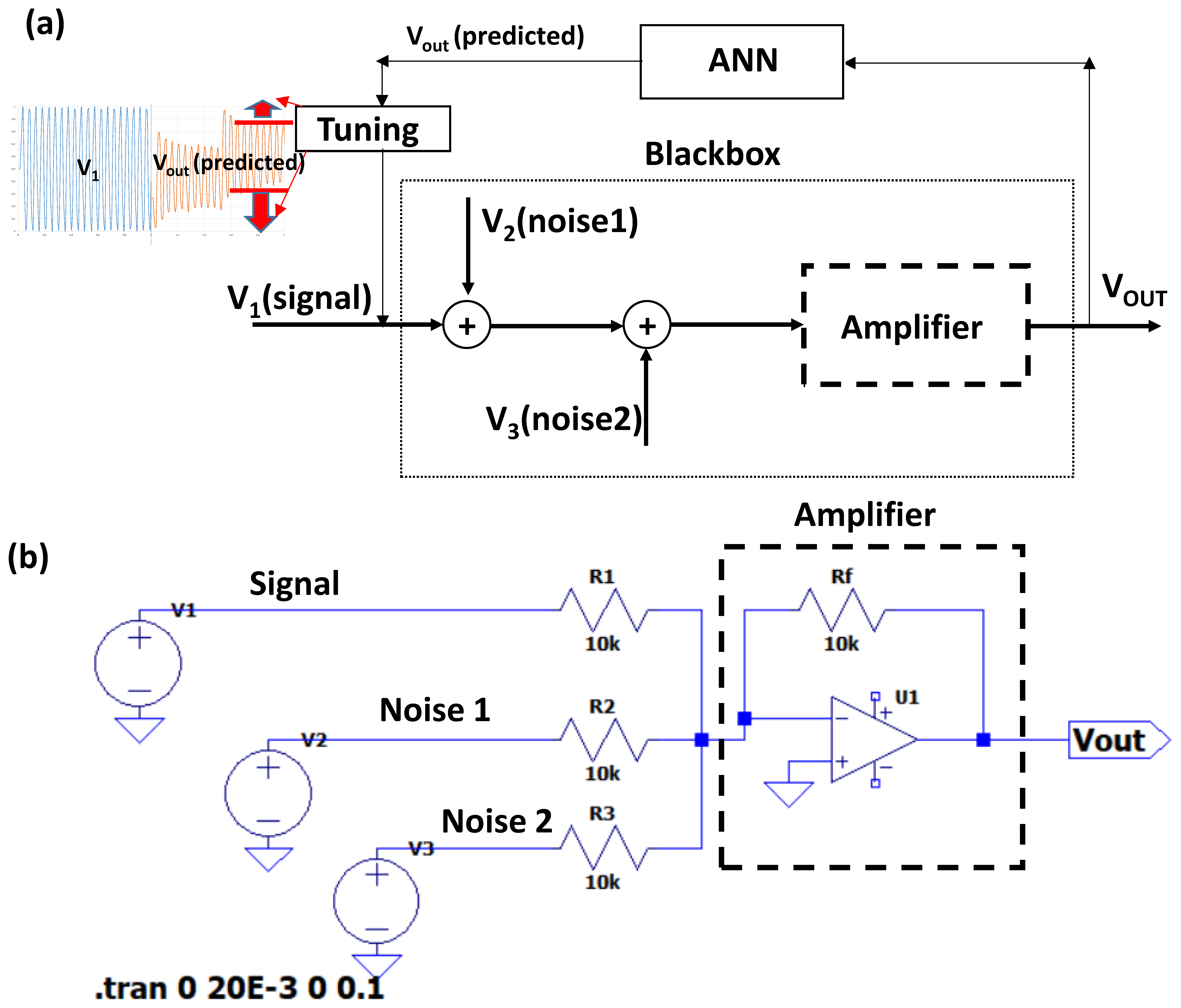
  • Input signal (V1): pure sinusoidal signal with f of 1 kHz, Voffset = 1 Volts, and Vamp = 2 Volts;
  • Noise (a): sinusoidal pulse signal with f of 1 kHz, Td = 10−2 s, ϑ = 500 s−1, φ = 45 deg., and Vamp = 2 Volts;
  • Noise (b): sinusoidal pulse signal with f of 1 kHz, Td = 0 s, ϑ = 500 s−1, φ = 45 deg., and Vamp = 2 Volts;
  • Noise (c): sinusoidal pulse signal with f of 4 kHz, Td = 0.002 s, ϑ = 0 s−1, φ = 0 deg., and Vamp = 2.4 Volts;
  • Noise (d): sinusoidal pulse signal with f of 4 kHz, Td = 0.008 s, ϑ = 500 s−1, φ = 45 deg., and Vamp = 2 Volts;
  • Noise (e): sinusoidal pulse signal with f of 3.3 kHz, Td = 0.003 s, ϑ = 0 s−1, φ = 0 deg., and Vamp = 2.4 Volts;
  • Noise (f): sinusoidal pulse signal with f of 1 kHz, Td = 0.008 s, ϑ = 500 s−1, φ = 45 deg., and Vamp = 2 Volts;
  • Noise (g): sinusoidal pulse signal with f of 8 kHz, Td = 0.002 s, ϑ = 0 s−1, φ = 0 deg., and Vamp = 2.4 Volts;
  • Noise (h): sinusoidal pulse signal with f of 8 kHz, Td = 0.008 s, ϑ = 500 s−1, φ = 45 deg., and Vamp = 2 Volts.
The performed simulation of the circuit of Figure 1b follows the configuration of Table 1.
The simulations are performed using the LTspice tool, a SPICE-based analog electronic circuit simulator open-source software [29] (Version x64: 24.0.11) providing time domain (transient analysis) and frequency domain results. The frequency domain results are executed using the LTspice Fast Fourier Transform (FFT) plugin. The FFT is an optimized algorithm for the implementation of the Discrete Fourier Transformation (DFT), allowing for faster data computation. DFT transforms a sequence of N numbers (time domain samples):
x N = x 0 , x 1   , ,   x N 1
to a sequence of another set of complex numbers:
X K = X 0 , X 1   , ,   X N 1
DFT using FFT can be written using the following formula:
X k = 1 n n = 0 N 1 x n · e j 2 π n k n
where N is the size of the domain for the results of the sum of a value n.
The output data (Vout) obtained by adding noises (see simulation configuration of Table 1) are locally imported by the Konstanz Miner (KNIME) [30] workflow of Figure 2 executing the ANN Vout prediction. Specifically, the workflow of Figure 2 is structured through the macro-functions of:
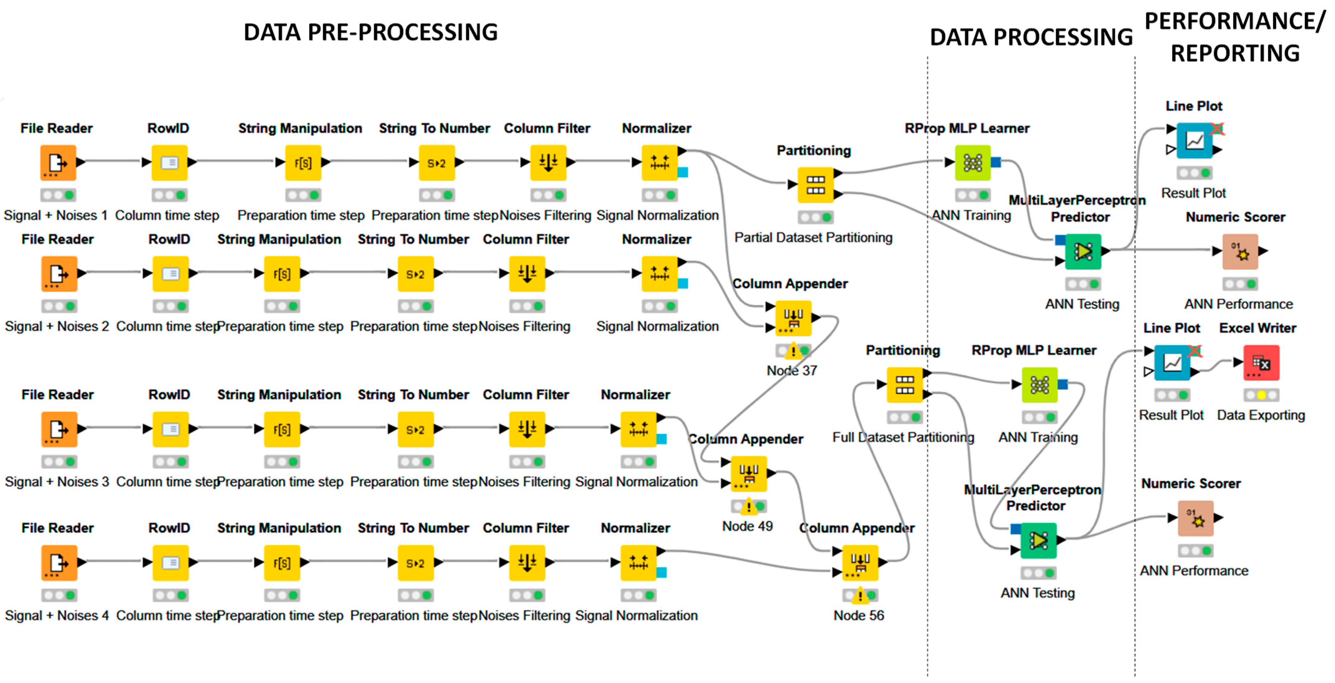
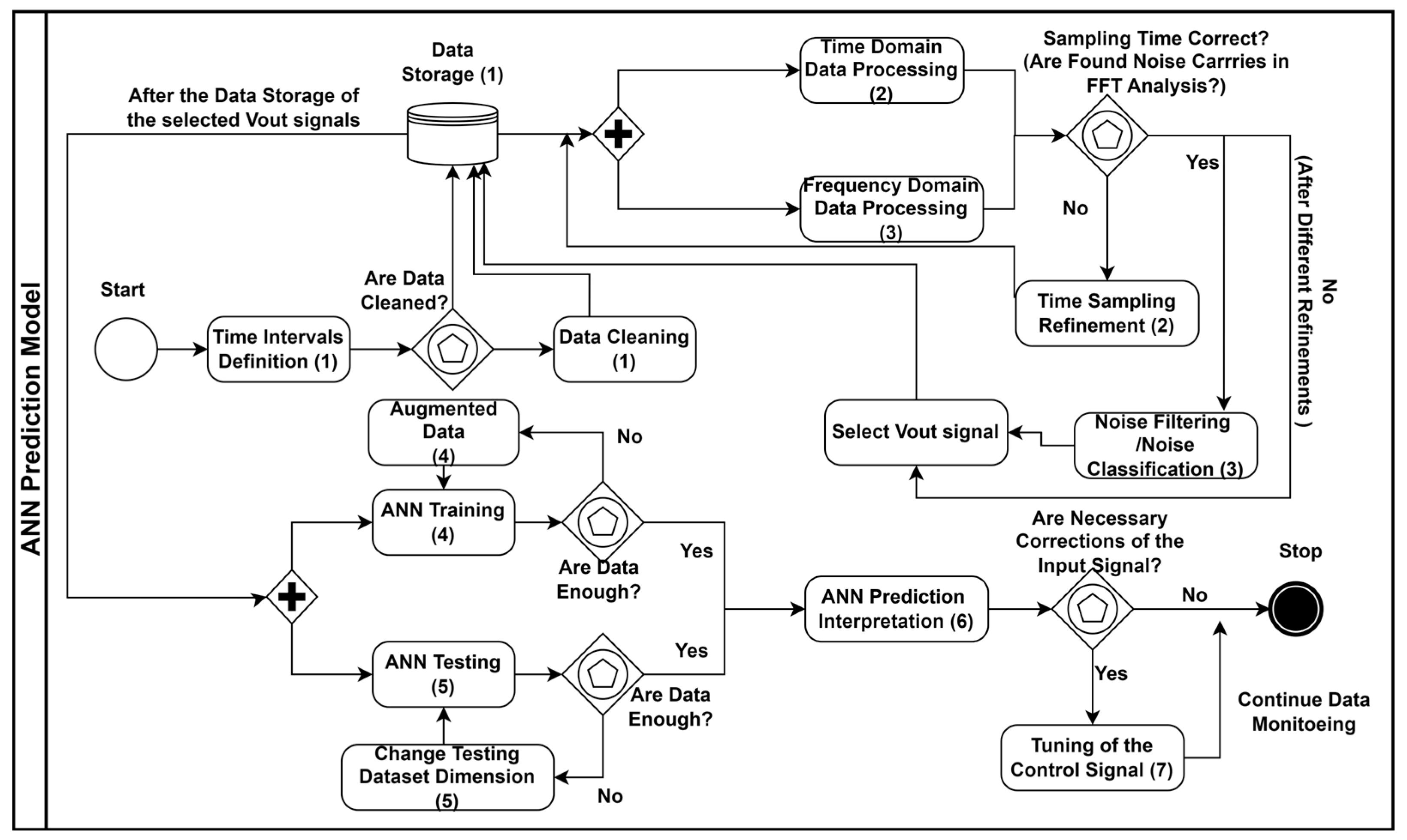
  • Data pre-processing: data importing in local repository, data manipulation, and data filtering;
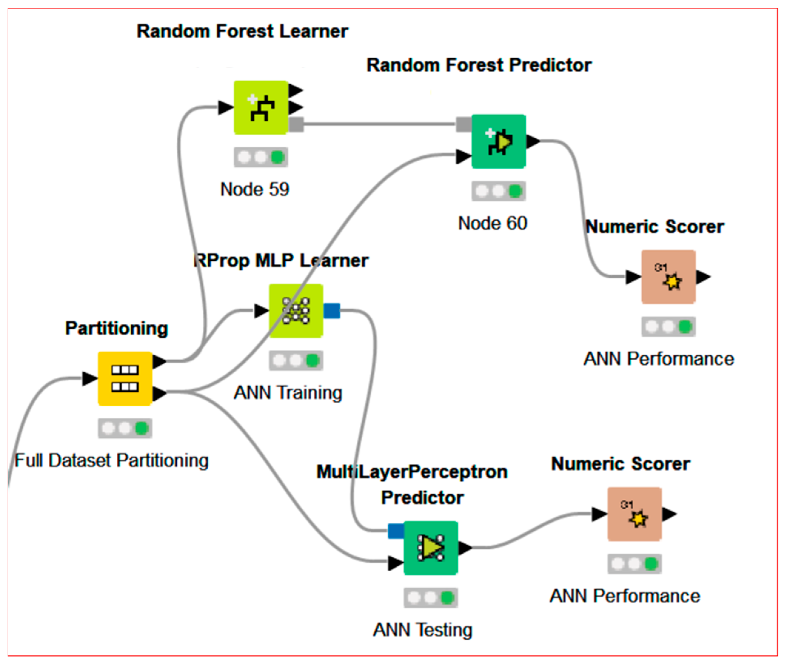
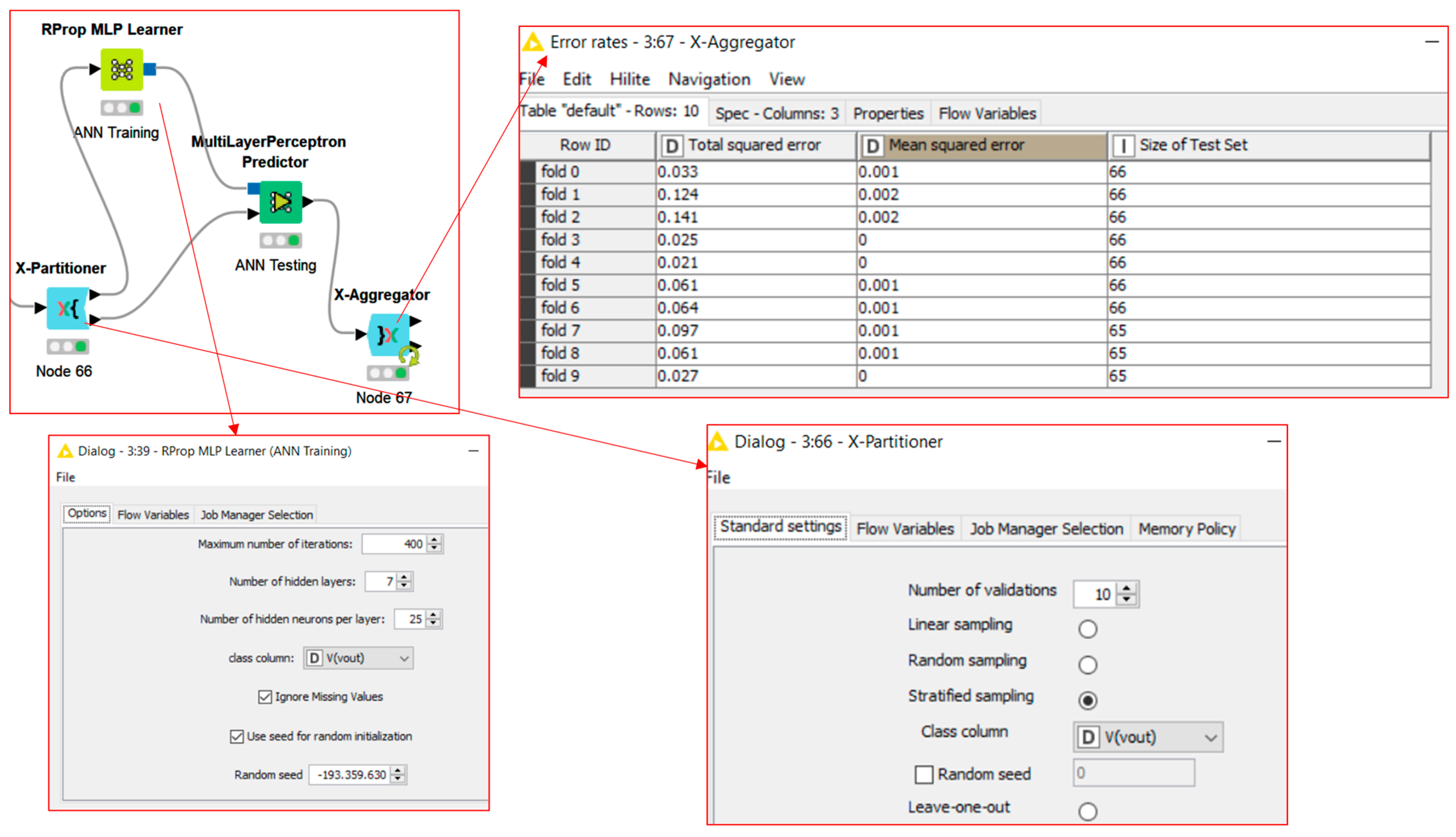
  • Data processing: ANN training and ANN testing models;
  • Data output: data visualization, algorithm performance scoring, and data exporting.
Figure 2. KNIME workflow predicting Vout signals of the circuit of Figure 1b.
Ai 05 00027 g002
The blocks (named nodes) structuring the workflow are as follows:
-
‘File Reader’: importing the .txt values of the simulations (outputs of the LTspice tool);
-
‘RowID’: generating time attributes (time steps as new column);
-
‘String Manipulation’ and ‘String to Number’: setting of the time column to integer attribute type;
-
‘Column Filter’: selecting of only the time steps and Vout columns;
-
‘Normalize’: normalizing the Vout signal;
-
‘Partitioning’: partitioning of the dataset into training and testing dataset;
-
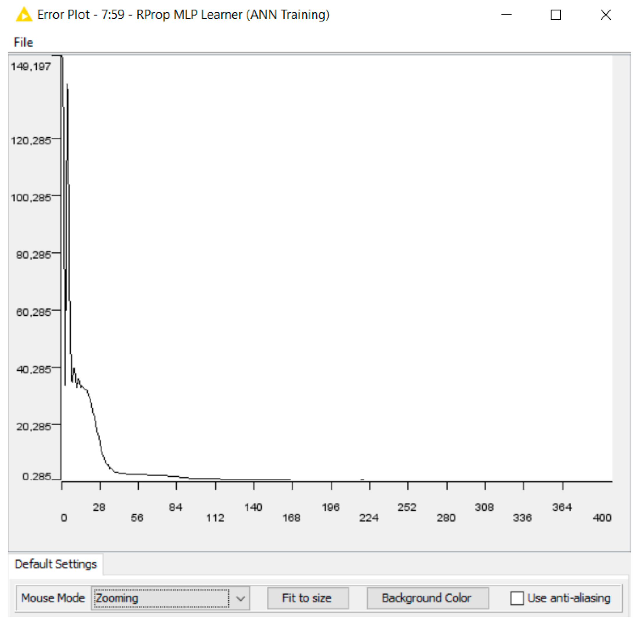
‘Rprop MLP Learner’: ANN training model based on Multilayer Perceptron (MLP) with adaptive RPROP algorithm [31];
-
‘Multilayer Perceptron Predictor’: testing the ANN-MLP model;
-
‘Column Appender’: appending different Vout signals of the simulations listed in Table 1;
-
‘Numeric Scorer’: evaluating ANN performance (R2, mean absolute error, mean squared error, root mean squared error, mean signed difference, mean absolute percentage error, adjusted R2);
-
‘Line Plot’: plotting of the prediction results;
-
‘Excel Writer’: exporting prediction results in excel file format to be plotted by other dashboards or data visualization plugins.
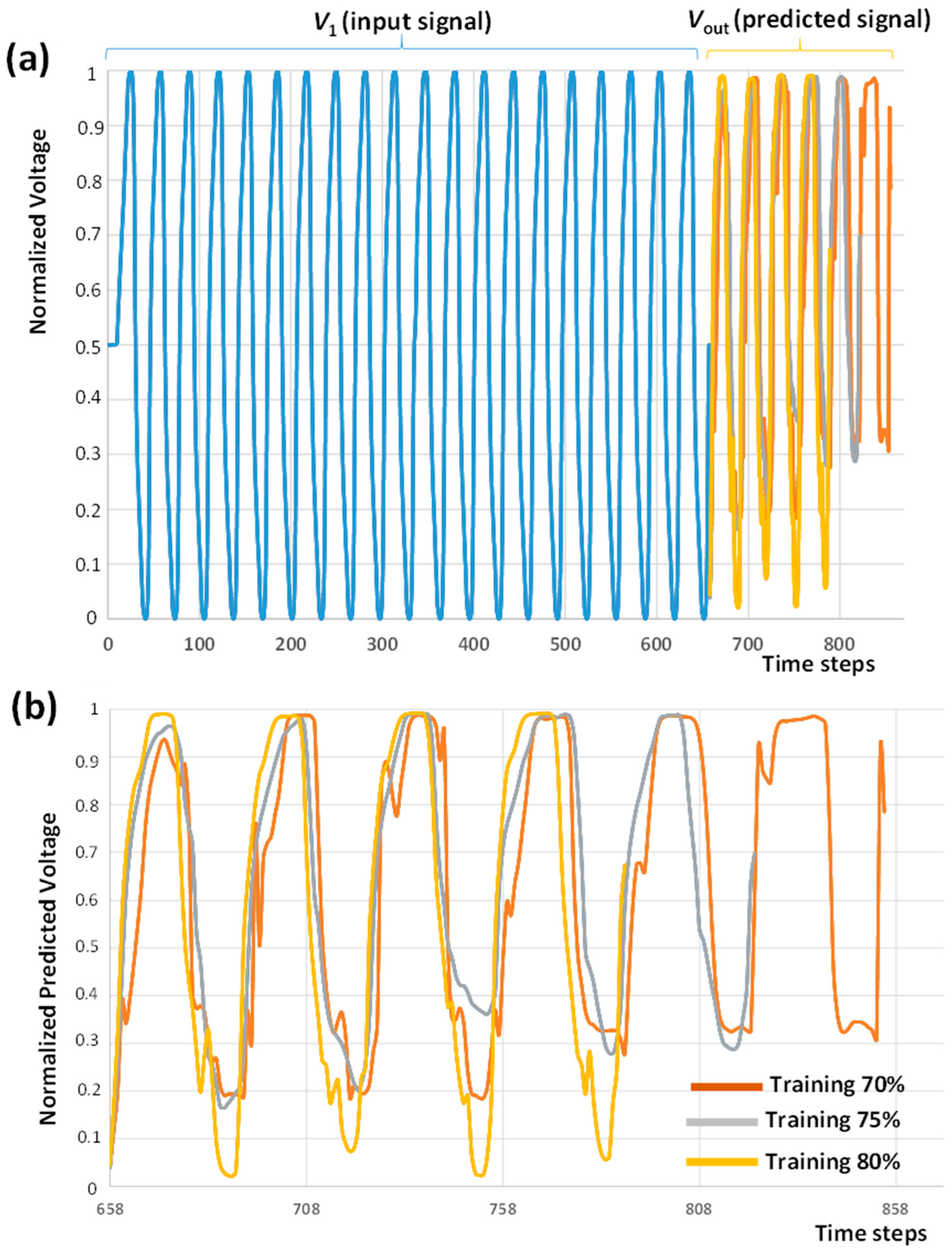
The modelling of the use criteria of the whole approach is sketched by the standard (ISO/IEC 19510:2013) Business Process Modeling and Notation (BPMN) graphical symbols using the open source Draw.io tool.

3. Results

The results proposed in this section are related to the following:
  • Ltspice simulation results (simulations of the circuit of Figure 1a configured as indicated in Table 1);
  • KNIME simulation predicting the noisy predicted Vout signals.

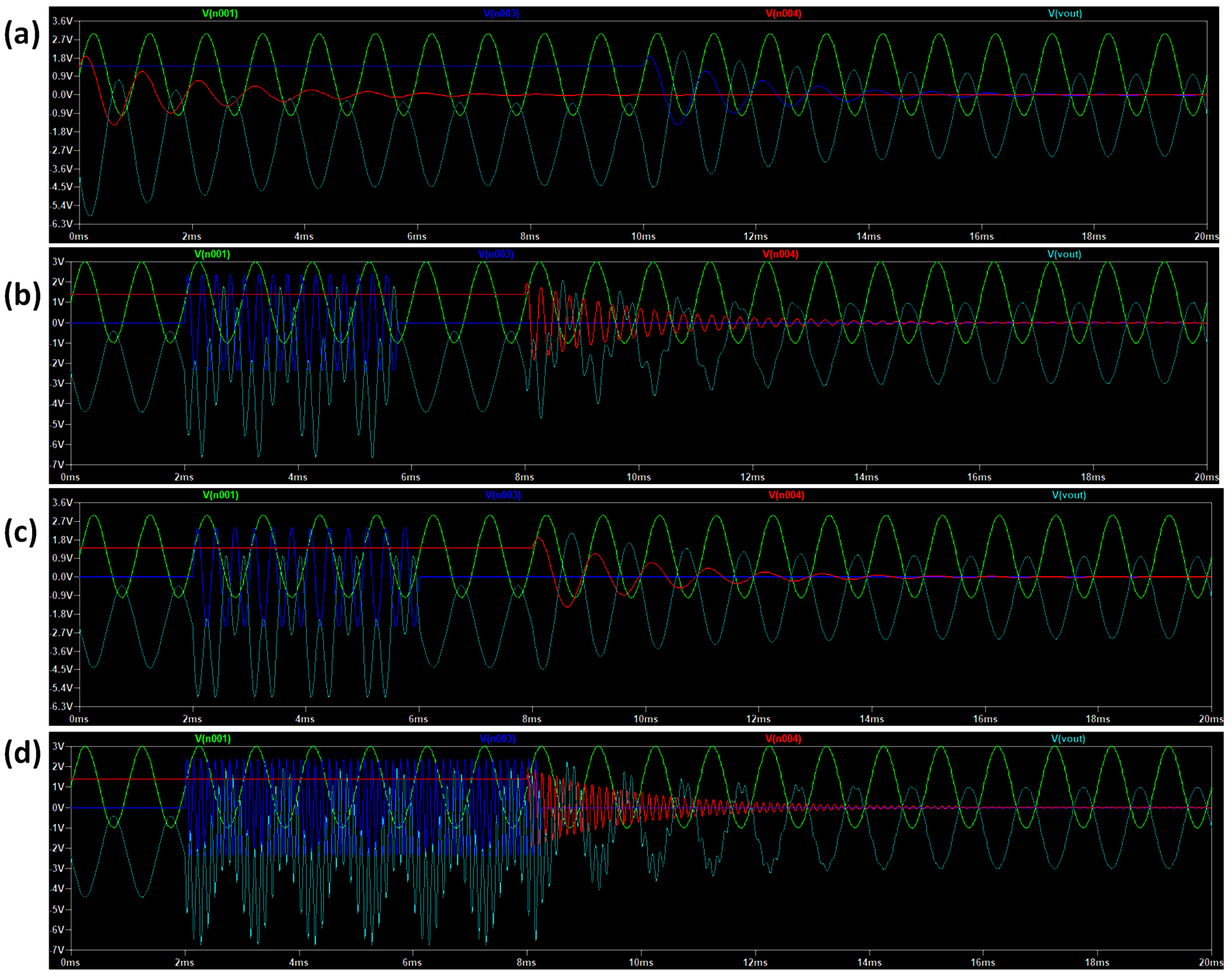
3.1. LTspice Results

The LTspice tool is applied to simulate the black box model of Figure 1b. A transient analysis is performed by using a stop time of 0.02 s, 0 s as the time to start saving data, and a maximum time step of 0.1 s. Figure 3 illustrates the time-domain of the four planned simulations combining the noises as planned in Table 1; each simulation takes into account three inputs of the operational amplifier of Figure 1b estimating the Vout signal. The additive inputs are the pure sinusoidal V1 signal and two noises signals distorting the input V1. The V1 is the desired output to be amplified behaving as a carrier controlling a machine or a processing tool (pure sinusoidal signal typically adopted for circuits controlled by a specific carrier).
An example of LTspice frequency analysis is illustrated in Appendix A: the Fast Fourier Transform (FFT) analysis compares the spectrum of the input signal V1 with the spectrum of a Vout signal disturbed by noises characterized by peaks in the frequency response. The results of Appendix A are a logarithmic graph with signal level (dB) on the vertical axis and frequency (Hz) on the horizontal axis representing the spectra values of Equation (5). By executing the four simulations of Table 1 independently, the output voltages signals (Vout) obtained are estimated as:
V o u t p u t t = ( V 1 t + N o i s e 1 t + N o i s e 2 t ) = ( V 1 t + V 2 t + V 3 t )
All the voltage calculated outputs constitute (with the input V1 signal and the time variable) the whole dataset to be processed by KNIME workflow of Figure 2 implementing the ANN algorithm.

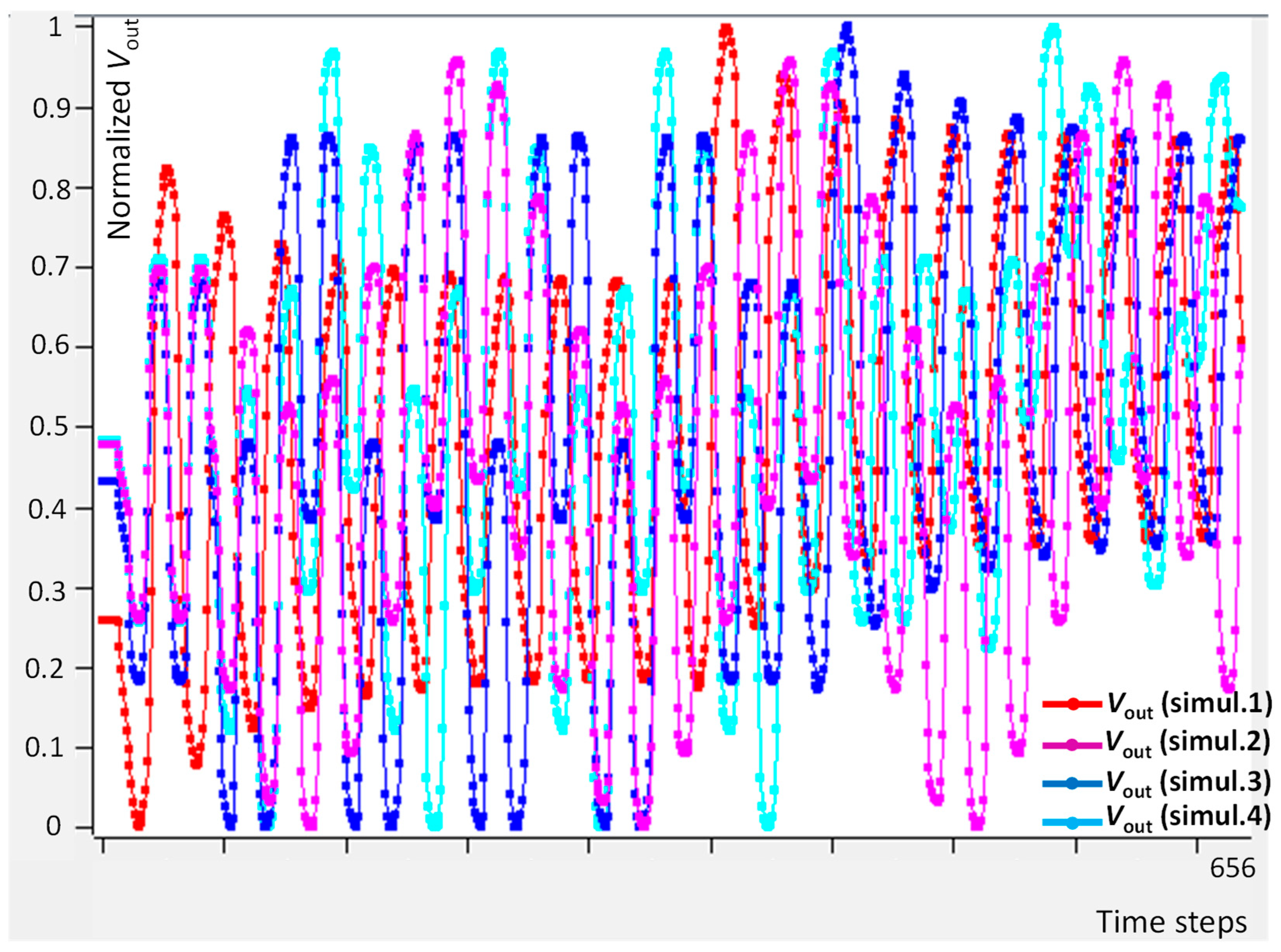
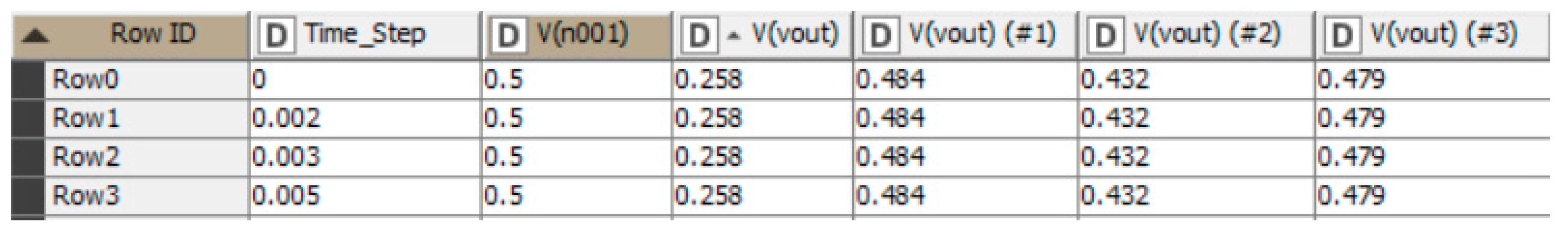
3.2. ANN Predicted Results

The dataset processed for the prediction of the noisy signal is formed by the four Vout signals of the simulations (see Figure 4), including the pure sinusoidal voltage V1 and the time step providing the temporal variation (times series forecasting application). Figure 5 illustrates a screenshot of the analyzed dataset having 657 records and 6 attributes (neural network input nodes) of the ANN.
The ANN-MLP network is configured to obtain the minimum calculus error fixing the following hyper-parameters: maximum number of iterations equals to 400, 7 hidden layers, and 25 as the number of hidden neurons per layer. The architecture of the optimized ANN-MLP model is sketched in Appendix B. As ANN results, Figure 6a illustrates the trend of the V1 input signal and predicted output signal Vout versus the time-step. The zoomed predicted Vout using different sizes of the training dataset (70%, 75% and 80%) is shown in Figure 6b. It is observed from Figure 6b that the predicted signal changes its trend with the size of the training dataset. Being the testing dataset extracted from the last values, and since the last values of Vout are not influenced by noises, the choice of the relative size of the training dataset of 70% provides the best prediction because the testing values are strongly influenced by noises. This aspect is clearly enhanced by observing the zooming of the predicted values in Figure 6b, highlighting the increasing trend of the minimum values of Vout.
The good performance of the ANN-MLP algorithm is proven by the error parameters estimated in Table 2, where the Random Forest (RF) performance (see the KNMIE workflow in Appendix B) is also indicated.
The procedure adopted for the choice of the ANN parameters is summarized in the following sequential steps: (1) the number of the hidden layers checking the minimum MAE error are varied; (2) then the epochs number at the minimum condition of step is varied before (1) verifying again the further minimum MAE for both step (1) and (2); (3) finally, it is set to the number of hidden neurons per layer, finding again the minimum MAE. For the analysis of step (2), the error plot trend (see Appendix B an example) is analyzed. Furthermore, it is observed that by choosing a training dataset partition of 80% (best partitioning providing the minimum error), the MAE error remains the same (MAE = 0.2) for testing dataset take from the last dataset values, selected linearly over the whole dataset, and using a random sampling. Further information about the cross-validation approach are in Appendix B.

4. Discussion

The prediction of the Vout signal of a controlling device provides useful information about possible complications in machine control. The proposed model highlights a methodology to estimate a predicted control signal at the output of an operational amplifier, modelling the amplification of all the signals (input signal and noises) behaving as a black box. The advantages and disadvantages of the proposed approach are mainly focused on the training of the ANN model, the predictive maintenance in case of strong input disturbances, machine tuning for possible intervention to enable, and on the cases of further complex noises influencing the final signal trend as multiplicative noises. The advantages and disadvantages of the ANN model are listed in Table 3.
By applying the ANN prediction, different limitations concern the computational time to perform real time data processing, the dataset availability, the efficiency of the training and testing datasets, and the possibility to classify correctly the noises affecting the control circuits. Important perspectives are found in augmented data and data cleaning techniques improving the training models, and in the use of advanced technologies such as quantum and edge computing. The perspectives are defined in advanced Industry 4.0/Industry 5.0 scenarios. The limitations and the perspectives of the ANN prediction are summarized in Table 4.
Despite these limitations, the study presents a novel approach to address a significant challenge in electronic circuit design and control systems. By treating the circuit as a “black box” and relying solely on input and output voltage signals, the proposed model offers a versatile solution that can adapt to various noise profiles and circuit configurations without requiring prior knowledge of the noise characteristics.
The drawback of the proposed black box model concerns the difficulty in understanding how the model generated the outputs; this generates further difficulties in identifying and correcting biases and other hyper-parameters for the training model. On the other hand, the main limitation is that the model is not transparent; this aspect causes possible errors of interpretations and, consecutively, uncertainties about the ANN accuracy.
The discussed method can be executed by distinguishing different sequential steps. Table 5 summarizes all six steps followed in the work and defines the use criteria, suggesting possible corrective actions optimizing a correct execution of the ANN model.
The disturbance signal profiles are considered sinusoidal components typically observed in power systems but also in low voltage ones [44,45,46,47]; harmonics sometimes referred to electromagnetic interferences and ‘electrical pollution’ characterizing complex electrical and electronic systems.
The use criteria, including possible corrective actions, listed in Table 5 are sketched by the BPMN model in Figure 7, indicating all the sequential steps followed in the modelling.
A practical application for the proposed approach is in the formulation of a digital twin specific for machine regulation and tuning for manufacturing processes, where the prediction of the output signal is fundamental to improve product quality decreasing defects. Future potential applications are in the integration of the ANN predictive model in advanced electronic systems of Industry 5.0, where AI algorithms are able to automate the machine setting according to the predicted output signal. Future research topics could be focused on the simultaneous analysis of time-domain and frequency-domain analyses.
In industrial scenarios, some examples of behaviors similar to the performed analysis are as follows: due switching (recurrent damped oscillating waves), lighting, operations in low voltage switchgears, energy transformation (presence of slot noises in generators), interferences (electromagnetic radiation), and injections of additional signals by different utilities.

5. Conclusions

This paper proposes an innovative ANN-based approach to predict the output voltage signal of amplifying circuits disturbed by noises. Specifically, by applying the black box concept, the model takes into account the typical effects of noises gained by an amplifier circuit predicting the noisy signal trend without knowing the noise typology. In order to test the ANN model, an ‘Adder’ circuit based on operational operator that is able to gain both input signal and noises is designed and simulated. The presented model could be extended to also predict irregular and chaotic noises, and it is suitable to structure a digital twin framework for Industry 5.0 scenarios, including intelligent automatisms and optimizing machine regulation procedures. Future research efforts could focus on validating the model’s performance across a broader range of circuit designs and noise conditions, as well as exploring its integration with existing control systems and automated tuning procedures. Additionally, investigating the model’s scalability and computational efficiency would be beneficial for its practical implementation in real-time monitoring and control applications.

Funding

This research received no external funding.

Institutional Review Board Statement

Not applicable.

Informed Consent Statement

Not applicable.

Data Availability Statement

Data are included in the paper.

Conflicts of Interest

The authors declare no conflicts of interest.

Appendix A

The FFT results of the input Voltage signal V1 are illustrated in Figure 1a, proving the presence of a frequency peak ad f = 1 kHz (carrier of the input signal). The influence of an additive noise is proven by the FFT analysis of the voltage output Vout of Figure A2, indicating the presence of a peak in f = 4 kHz (as noise © and noise (d)).
Figure A1. Example of a FFT input V1 signal. Inset: time domain trend of the input V1 signal (pure sinusoidal signal).
Ai 05 00027 g0a1
Figure A2. Example of a FFT output Vout signal effected by oscillating noises. Inset: time domain trend of the output Vout signal.
Ai 05 00027 g0a2

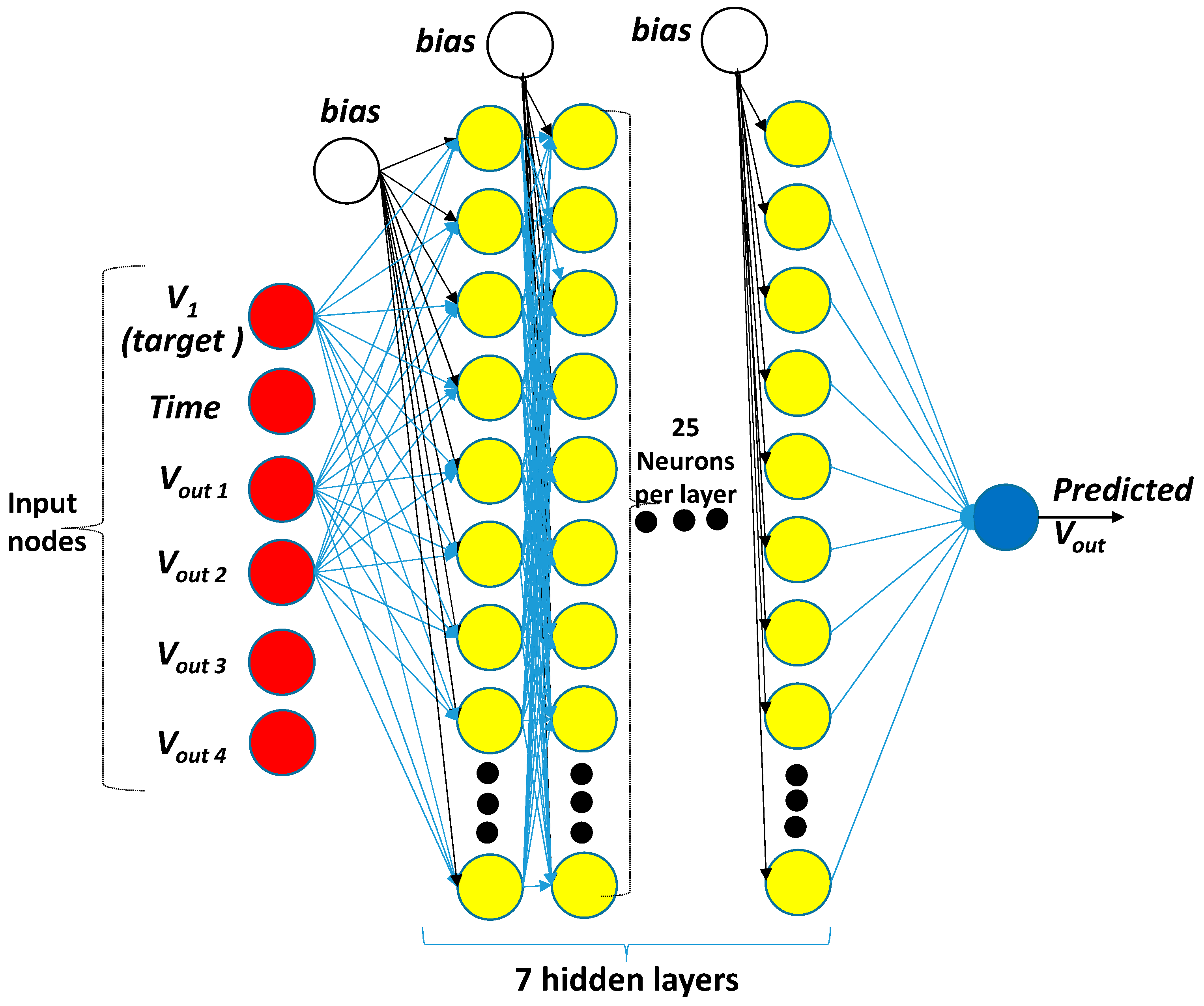
Appendix B. ANN Algorithm Architecture and Performance Aspects

The optimized ANN-MLP is selected by minimizing the error values indicated in Table 2. Illustrated in Figure A3 is the architecture of the optimized ANN-MLP network characterized by 4 input nodes with V1 labelled as a class (target). The optimized ANN-MLP network is characterized by 7 hidden layers and 25 neurons per layer.
Figure A3. Optimized neural ANN-MLP network predicting Vout signal.
Ai 05 00027 g0a3
Illustrated in Figure A4 is the error plot trend of the RProp MLP learner.
Figure A4. RProp MLP error trend versus the epochs number.
Ai 05 00027 g0a4
The cross-validation test is executed for the optimized ANN-MLP algorithm by using the ‘X-Partitioner’ and the ‘X-Aggregator’ blocks of KNIME blocks. The performed test cross-validation takes into account ten number of validations using a stratified sampling approach defining the ten test subsets to process named folds. For the specific case, an average MSE value of 0.001 is observed.
Figure A5. Screenshot of the cross-validation test applied to the optimized MLP algorithm.
Ai 05 00027 g0a5
Figure A6 illustrates the KNIME workflow adopted for the comparative analysis of Table 4.
Figure A6. Part of the KNIME workflow comparing performances between RF and ANN-MLP algorithms.
Ai 05 00027 g0a6

References

  1. Zhao, H.; Chen, Z.; Shu, X.; Shen, J.; Liu, Y.; Zhang, Y. Multi-Step Ahead Voltage Prediction and Voltage Fault Diagnosis Based on Gated Recurrent Unit Neural Network and Incremental Training. Energy 2023, 266, 126496. [Google Scholar] [CrossRef]
  2. Mokhtar, M.; Robu, V.; Flynn, D.; Higgins, C.; Whyte, J.; Loughran, C.; Fulton, F. Prediction of Voltage Distribution Using Deep Learning and Identified Key Smart Meter Locations. Energy AI 2021, 6, 100103. [Google Scholar] [CrossRef]
  3. Alsouda, Y.; Pllana, S.; Kurti, A. A Machine Learning Driven IoT Solution for Noise Classification in Smart Cities. arXiv 2018, arXiv:1809.00238. [Google Scholar]
  4. Alsouda, Y.; Pllana, S.; Kurti, A. IoT-Based Urban Noise Identification Using Machine Learning: Performance of SVM, KNN, Bagging, and Random Forest. In Proceedings of the International Conference on Omni-Layer Intelligent Systems, Crete, Greece, 5–7 May 2019; ACM: New York, NY, USA, 2019. [Google Scholar]
  5. Rahman, M.S.; Ghosh, T.; Aurna, N.F.; Kaiser, M.S.; Anannya, M.; Hosen, A.S.M.S. Machine Learning and Internet of Things in Industry 4.0: A Review. Measur. Sens. 2023, 28, 100822. [Google Scholar] [CrossRef]
  6. Lo Brano, V.; Ciulla, G.; Di Falco, M. Artificial Neural Networks to Predict the Power Output of a PV Panel. Int. J. Photoenergy 2014, 2014, 193083. [Google Scholar] [CrossRef]
  7. Shingare, S.S.; Khampariya, P.; Bakre, S.M. Efficient Fault Detection and Location in Extra High Voltage Networks: An Artificial Neural Network (ANN)-Based Approach. Int. J. Intell. Syst. Appl. Eng. 2023, 11, 1051–1060. [Google Scholar]
  8. Ogar, V.N.; Hussain, S.; Gamage, K.A.A. The Use of Artificial Neural Network for Low Latency of Fault Detection and Localisation in Transmission Line. Heliyon 2023, 9, e13376. [Google Scholar] [CrossRef]
  9. Rosa, J.P.S.; Guerra, D.J.D.; Horta, N.C.G.; Martins, R.M.F.; Lourenço, N.C.C. Using Artificial Neural Networks for Analog Integrated Circuit Design Automation; Springer International Publishing: Cham, Switzerland, 2020. [Google Scholar]
  10. Massaro, A. Electronics in Advanced Research Industries: Industry 4.0 to Industry 5.0 Advances; Wiley: Hoboken, NJ, USA, 2021. [Google Scholar]
  11. Massaro, A. Intelligent Materials and Nanomaterials Improving Physical Properties and Control Oriented on Electronic Implementations. Electronics 2023, 12, 3772. [Google Scholar] [CrossRef]
  12. Arabi, A.; Ayad, M.; Bourouba, N.; Benziane, M.; Griche, I.; Ghoneim, S.S.M.; Ali, E.; Elsisi, M.; Ghaly, R.N.R. An Efficient Method for Faults Diagnosis in Analog Circuits Based on Machine Learning Classifiers. Alex. Eng. J. 2023, 77, 109–125. [Google Scholar] [CrossRef]
  13. Sobanski, P.; Kaminski, M. Application of Artificial Neural Networks for Transistor Open-circuit Fault Diagnosis in Three-phase Rectifiers. IET Power Electron. 2019, 12, 2189–2200. [Google Scholar] [CrossRef]
  14. Zhao, T.; Wei, J.; Lan, B.; Peng, Q.; Wan, J. A Unified Black-box Macro Model for Analog Circuit Based on Artificial Neural Network. Int. J. Circuit Theory Appl. 2023, 51, 4455–4464. [Google Scholar] [CrossRef]
  15. Yarikkaya, S.; Vardar, K. Neural Network Based Predictive Current Controllers for Three Phase Inverter. IEEE Access 2023, 11, 27155–27167. [Google Scholar] [CrossRef]
  16. Vargas, F.; Borba, D.; Benfica, J.D.; Syed, R.T. Artificial Neural Network Accelerator for Classification of In-Field Conducted Noise in Integrated Circuits’ DC Power Lines. In Proceedings of the 2023 IEEE 29th International Symposium on On-Line Testing and Robust System Design (IOLTS), Crete, Greece, 3–5 July 2023; pp. 1–6. [Google Scholar]
  17. Ferdous, H.; Jahan, S.; Tabassum, F.; Islam, M.I. The performance analysis of digital filters and ANN in DE-noising of speech and biomedical signal. Int. J. Image Graph. Signal Process. 2023, 1, 63–78. [Google Scholar] [CrossRef]
  18. Dieste-Velasco, M.I.; Diez-Mediavilla, M.; Alonso-Tristán, C. Regression and ANN Models for Electronic Circuit Design. Complexity 2018, 2018, 7379512. [Google Scholar] [CrossRef]
  19. Mina, R.; Jabbour, C.; Sakr, G.E. A Review of Machine Learning Techniques in Analog Integrated Circuit Design Automation. Electronics 2022, 11, 435. [Google Scholar] [CrossRef]
  20. Kouhalvandi, L.; Guerrieri, S.D. Modeling of HEMT Devices through Neural Networks: Headway for Future Remedies. In Proceedings of the 2023 10th International Conference on Electrical and Electronics Engineering (ICEEE), Istanbul, Turkiye, 8–10 May 2023; pp. 261–267. [Google Scholar]
  21. Gao, Z.; Yan, S.; Zhang, J.; Mascarenhas, M.; Nejabati, R.; Ji, Y.; Simeonidou, D. ANN-Based Multi-Channel QoT-Prediction over a 563.4-Km Field-Trial Testbed. J. Lightwave Technol. 2020, 38, 2646–2655. [Google Scholar] [CrossRef]
  22. Marinković, Z.; Crupi, G.; Caddemi, A.; Marković, V.; Schreurs, D.M.M.-P. A Review on the Artificial Neural Network Applications for Small-signal Modeling of Microwave FETs. Int. J. Numer. Model. 2020, 33, e2668. [Google Scholar] [CrossRef]
  23. Marinković, Z.; Pronić-Rančić, O.; Marković, V. Small-Signal and Noise Modeling of Class of HEMTs Using Knowledge-Based Artificial Neural Networks. Int. J. RF Microw. Comput-Aid. Eng. 2013, 23, 34–39. [Google Scholar] [CrossRef]
  24. Zur, R.M.; Jiang, Y.; Pesce, L.L.; Drukker, K. Noise Injection for Training Artificial Neural Networks: A Comparison with Weight Decay and Early Stopping. Med. Phys. 2009, 36, 4810–4818. [Google Scholar] [CrossRef]
  25. Lee, C.-I.; Lin, Y.-T.; Lin, W.-C. Improved Artificial Neural Network RF Noise Model for MOSFETs Operating in Avalanche Region. Electron. Lett. 2016, 52, 232–234. [Google Scholar] [CrossRef]
  26. Amaral, A.; Gusmão, A.; Vieira, R.; Martins, R.; Horta, N.; Lourenço, N. An ANN-Based Approach to the Modelling and Simulation of Analogue Circuits. In Proceedings of the 2023 19th International Conference on Synthesis, Modeling, Analysis and Simulation Methods and Applications to Circuit Design (SMACD), Funchal, Portugal, 3–5 July 2023; pp. 1–4. [Google Scholar]
  27. Litovski, V. 5.4 Low-Noise Amplifiers. In Lecture Notes in Electrical Engineering; Springer Nature: Singapore, 2024; pp. 91–141. [Google Scholar]
  28. Cornell University. An Active Noise Canceler to Eliminate the 60 Hz Noise Found in Electrical Signals Due to AC Power-Line Contamination. Available online: https://people.ece.cornell.edu/land/courses/ece4760/FinalProjects/s2008/rmo25_kdw24/rmo25_kdw24/index.html#references (accessed on 13 April 2024).
  29. LTspice. Available online: https://www.analog.com/en/resources/design-tools-and-calculators/ltspice-simulator.html (accessed on 13 April 2024).
  30. KNIME. Available online: https://www.knime.com/ (accessed on 13 April 2024).
  31. Riedmiller, M.; Braun, H. A Direct Adaptive Method for Faster Backpropagation Learning: The RPROP Algorithm. In Proceedings of the IEEE International Conference on Neural Networks, Honolulu, HI, USA, 12–17 May 2002; Volume 1, pp. 586–591. [Google Scholar]
  32. Ding, J.; Peres, Y.; Ranade, G.; Zhai, A. When Multiplicative Noise Stymies Control. Ann. Appl. Probab. 2019, 29, 1963–1992. [Google Scholar] [CrossRef]
  33. Monjur, M.M.R.; Heacock, J.; Calzadillas, J.; Mahmud, M.D.S.; Roth, J.; Mankodiya, K.; Sazonov, E.; Yu, Q. Hardware Security in Sensor and Its Networks. Front. Sens. 2022, 3, 850056. [Google Scholar] [CrossRef]
  34. Monjur, M.R.; Sunkavilli, S.; Yu, Q. ADobf: Obfuscated Detection Method against Analog Trojans on I2C Master-Slave Interface. In Proceedings of the 2020 IEEE 63rd International Midwest Symposium on Circuits and Systems (MWSCAS), Springfield, MA, USA, 9–12 August 2020; pp. 1064–1067. [Google Scholar]
  35. Monjur, M.; Calzadillas, J.; Yu, Q. Hardware Security Risks and Threat Analyses in Advanced Manufacturing Industry. ACM Trans. Des. Automat. Electron. Syst. 2023, 28, 1–22. [Google Scholar] [CrossRef]
  36. Zhou, G.; Zhang, C.; Li, Z.; Ding, K.; Wang, C. Knowledge-Driven Digital Twin Manufacturing Cell towards Intelligent Manufacturing. Int. J. Prod. Res. 2020, 58, 1034–1051. [Google Scholar] [CrossRef]
  37. Abdoune, F.; Cardin, O.; Nouiri, M.; Castagna, P. Real-Time Field Synchronization Mechanism for Digital Twin Manufacturing Systems. IFAC 2023, 56, 5649–5654. [Google Scholar] [CrossRef]
  38. Soori, M.; Arezoo, B.; Dastres, R. Digital Twin for Smart Manufacturing, A Review. Sustain. Manuf. Serv. Econ. 2023, 2, 100017. [Google Scholar] [CrossRef]
  39. Massaro, A. Advanced Electronic and Optoelectronic Sensors, Applications, Modelling and Industry 5.0 Perspectives. Appl. Sci. 2023, 13, 4582. [Google Scholar] [CrossRef]
  40. Subramaniam, S.R.; Georgakis, A. A Simple Filter Circuit for Denoising Biomechanical Impact Signals. In Proceedings of the 2009 Annual International Conference of the IEEE Engineering in Medicine and Biology Society, Minneapolis, MN, USA, 3–6 September 2009; pp. 6938–6941. [Google Scholar]
  41. Yu, F.-M.; Lee, K.-C.; Jwo, K.-W.; Chang, R.-S.; Lin, J.-Y. Low Distortion of Noise Filter Realization with 6.34 V/Μs Fast Slew Rate and 120 mVp-p Output Noise Signal. Sensors 2021, 21, 1008. [Google Scholar] [CrossRef]
  42. Lyu, P.; Zhang, H.; Yu, W.; Liu, C. A Novel Model-Independent Data Augmentation Method for Fault Diagnosis in Smart Manufacturing. Procedia CIRP 2022, 107, 949–954. [Google Scholar] [CrossRef]
  43. Massaro, A. Multi-Level Decision Support System in Production and Safety Management. Knowledge 2022, 2, 682–701. [Google Scholar] [CrossRef]
  44. Lovisolo, L.; Tcheou, M.P.; da Silva, E.A.B.; Rodrigues, M.A.M.; Diniz, P.S.R. Modeling of Electric Disturbance Signals Using Damped Sinusoids via Atomic Decompositions and Its Applications. EURASIP J. Adv. Signal Process. 2007, 029507. [Google Scholar] [CrossRef]
  45. Cordero, R.; Estrabis, T.; Gentil, G.; Caramalac, M.; Suemitsu, W.; Onofre, J.; Brito, M.; dos Santos, J. Tracking and Rejection of Biased Sinusoidal Signals Using Generalized Predictive Controller. Energies 2022, 15, 5664. [Google Scholar] [CrossRef]
  46. Liu, Y.-J.; Chen, C.-I.; Fu, W.-C.; Lee, Y.-D.; Cheng, C.-C.; Chen, Y.-F. A Hybrid Approach for Low-Voltage AC Series Arc Fault Detection. Energies 2023, 16, 1256. [Google Scholar] [CrossRef]
  47. Monedero, I.; Leon, C.; Ropero, J.; Garcia, A.; Elena, J.M.; Montano, J.C. Classification of Electrical Disturbances in Real Time Using Neural Networks. IEEE Trans. Power Deliv. 2007, 22, 1288–1296. [Google Scholar] [CrossRef]
Figure 1. (a) Theoretical black box model of a signal amplification influenced by added noises and ANN data processing to adjust the input signal (for example, by tuning in advance the signal amplitude). (b) LTspice circuit modelling the black box scheme of Figure 1a.
Ai 05 00027 g001
Figure 3. LTspice simulations of the configurations of Table 1: (a) simulation 1; (b) simulation 2; (c) simulation 3; (d) simulation 4. The pure sinusoidal input V1 is the green plot.
Ai 05 00027 g003
Figure 4. ANN input dataset constructed by storing all the Vout signals obtained from the four simulations. The plots are extracted from the results of Figure 3.
Ai 05 00027 g004
Figure 5. KNIME normalized dataset processed by the ANN workflow.
Ai 05 00027 g005
Figure 6. (a) V1 input signal and predicted output signal Vout versus the time-step. (b) Zoomed predicted Vout using different sizes of the training dataset (70%, 75%, and 80%).
Ai 05 00027 g006
Figure 7. Use criteria of the proposed model modelled by the BPMN notation.
Ai 05 00027 g007
Table 1. Simulation configurations of the black box model of Figure 1b.
SimulationV2 (Noise 1 of Figure 1b)V3 (Noise 2 of Figure 1b)
Simulation 1Noise (a)Noise (b)
Simulation 2Noise (c)Noise (d)
Simulation 3Noise (e)Noise (f)
Simulation 4Noise (g)Noise (h)
Table 2. ANN-MLP performance parameters of the optimized algorithm versus RF algorithm.
ParameterANN-MLPRF
R20.960.96
Mean Absolute Error (MAE)0.020.031
Mean Squared Error (MSE)0.0010.002
Root Mean Squared Error (RMSE)0.0340.039
Mean Signed Difference (MSD)0.0210.014
Mean Absolute Percentage Error0.0540.062
Table 3. Main advantages and disadvantages of the ANN prediction of the noisy signal in manufacturing industries.
ANN Prediction AspectsAdvantagesDisadvantages
ANN training modelPossibility to construct the training model by considering the historical output data of the circuits without knowing the noisy profile (black box behavior).A good training requires a dataset including all the potential noises which could influence the output signal (a long time is required to store information about the impact of probable noises).
Predictive MaintenanceThe prediction of a strong noisy signal trend could enable predictive maintenance processes avoiding machine breakage.Difficulty to distinguish dangerous noisy signals to enable the predictive maintenance procedures.
Machine tuningThe signal trend prediction allows for the automation of the input signal setting, thus anticipating corrective actions. A feedback system controlled by an AI engine could optimize the parameter setting generating a new input signal correcting control errors [10].A correct machine tuning is performed when probable noises are considered. New typologies of disturbs or noises not included as historical Vout could provide wrong predictions and, consequently, wrong tuning or parameter setting.
Multiplicative noisesThe ANN prediction is adaptable also when unwanted random signals are multiplied into machine control inputs [32].The error prediction increases with the complexity of noises as for multiplicative noises.
Intentional manumissionThe prediction of possible noisy trend is important also to find possible hardware analog Trojans [33,34,35].Difficulty to distinguish the hardware attacks to noises and disturbs intrinsic of machinery.
Digital Twin (DT)The proposed approach is suitable to developing DT models [36,37,38] simulating the behavior of whole production lines in manufacturing industries.DT models could be approximate and not match with the real behavior of the production processes.
Table 4. Limitations and perspectives of ANN predictions in Industry 4.0/Industry 5.0 scenarios.
Technological LimitsTechnology DescriptionTechnological Perspectives
Real time predictionThe time delay of the data processing defines a quasi-real data processing. Strong delays are possible for big data processing.Some advanced technologies such as edge computing or quantum computing [39] could be adopted for a real time data processing computing massive datasets.
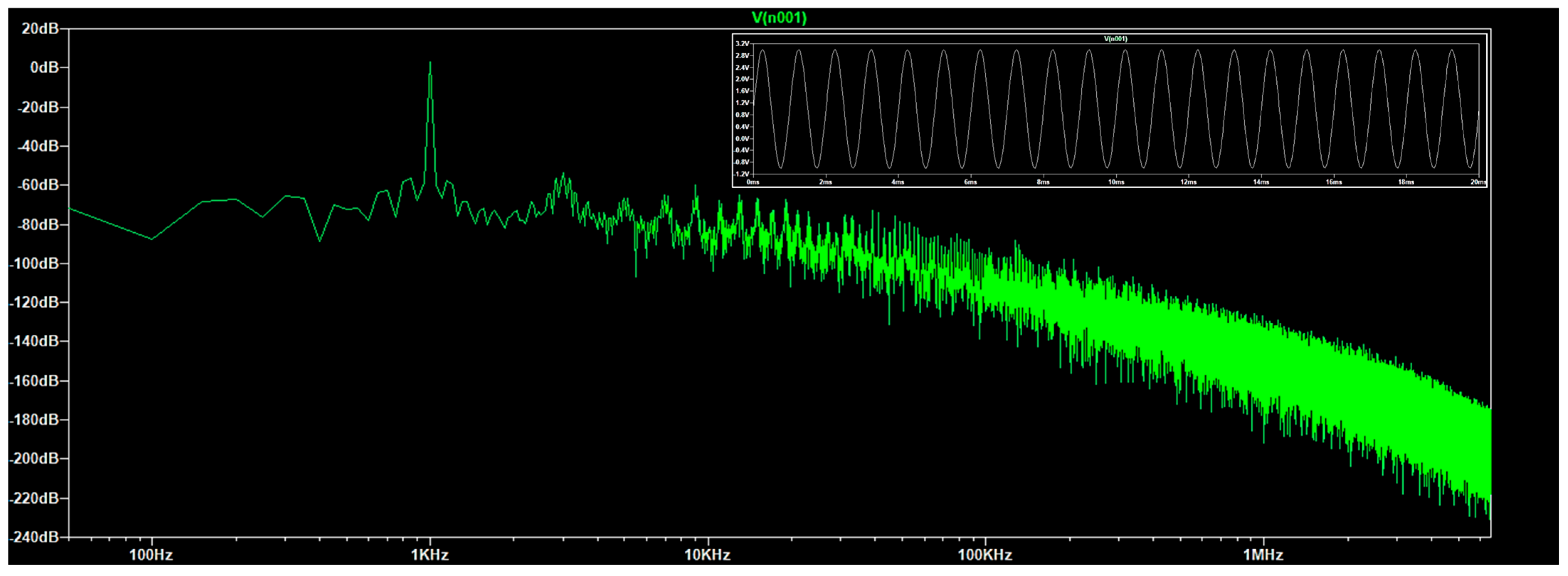
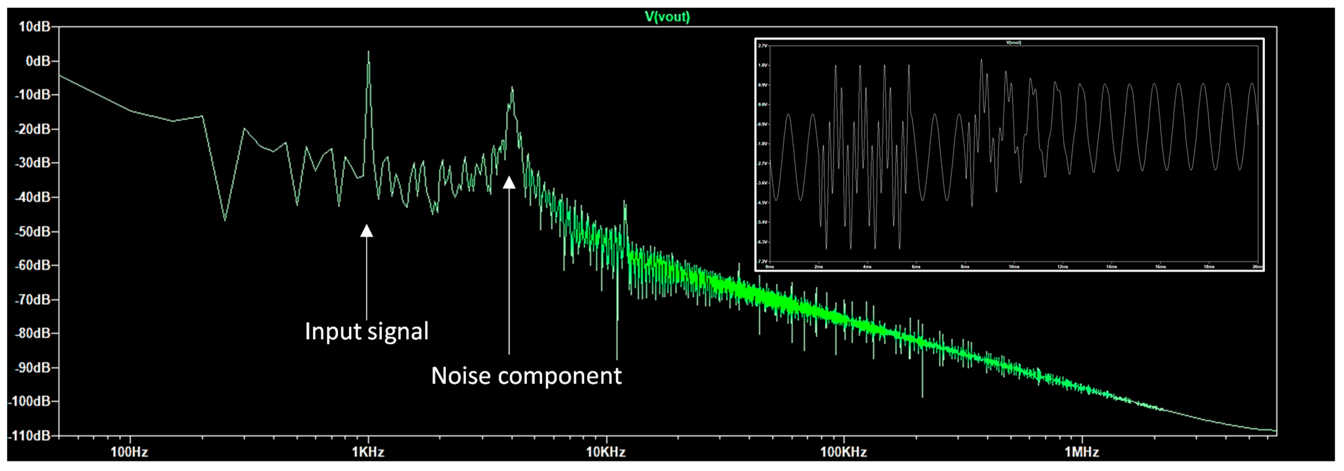
Knowledge of the noise spectraGenerally, the noises knowledge is missing: both time domain profile and frequency spectrum are unknown. Some useful information is possible to obtain for noises characterized by a carrier which is visible in the whole spectrum of the output signal (see Appendix A).Machine learning supervised algorithms could be applied to also predict the behavior of the output signal in the frequency domain by applying denoising filtering approaches [40,41].
Dataset availabilityThe data availability are fundamental for data processing of machine learning supervised algorithms requiring a large number of cleaned data to optimize the training model.Some methodologies such as augmented data [42] could be adopted to increase the dataset.
Automated Controlling Systems (ACS)The big data processing requires a high computational cost generating delays or interrupts before to execute the decision-making automatic systems less effective.A specific calculus engine could be used to increase the efficiency of the automated controlling systems.
Testing datasetThe testing dataset (last values of Vout signals) could be not influenced by noises and, consecutively, the prediction could be partially wrong.Other techniques for the extraction of the testing model (such as linear sampling or random sampling) could include with a greater probability the noisy behavior.
Training datasetThe training dataset should include a variety of probable noises.The historical dataset could be selected by eliminating redundancies and longtime of regular signal (pre-filtering approach of the training dataset).
Classification of the single noiseWhen many noises influence the output signal, it is very difficult to classify each noise signal.Due to the difficulty to classify and filter the single noise, it is possible in advance to tune or adjust the profile of the whole signal output.
Table 5. Use criteria of the proposed model and possible corrective actions deduced from the analysis.
Function of the Model (Sequential Steps)Use CriteriaPossible Corrective Actions
1-
Data storage
Definition of the time intervals to detect and store data outputs.Cleaning of the dataset (filtering of wrong data or missing values).
2-
Time domain data processing
Definition of the accuracy of the sampling (sampling time step definition).Decrease in the sampling time to store also highly variable noises.
3-
Frequency domain data processing
Frequency analysis matching with the time domain one to find possible noises characterized by carriers: the trend of the output predicted signals are compared with the FFT spectra to extract information about possible carries thus supporting noise classification.Application of narrow filters to suppress undesired carriers.
4-
Data training pre-processing
Creation of the ANN training model by considering different voltage output.Use of augmented data to increase the efficiency of the training model.
5-
Choice of the data testing model
Selection of the testing dataset possibly including the noise effects.Change in the testing dataset dimension to include possible noises.
6-
ANN data prediction interpretation
Analysis and interpretation of the predicted output signals.Possible corrective actions are defined by considering priorities and multi-level Decision Support Systems (DSSs) [43].
7-
Tuning approach
Tuning of the input signals matching with ANN data prediction interpretation by acting on the input signal (regulation of the input signal or adding of further control signal).Use of denoising filters according with the predicted output trend and with the FFT responses (suppression of undesired carriers). Modification of the input signal combining other input signals able to correct the minimum and the maximum amplitude of the output signal.
Disclaimer/Publisher’s Note: The statements, opinions and data contained in all publications are solely those of the individual author(s) and contributor(s) and not of MDPI and/or the editor(s). MDPI and/or the editor(s) disclaim responsibility for any injury to people or property resulting from any ideas, methods, instructions or products referred to in the content.

