
Software Defect Prediction Based on Machine Learning and Deep Learning Techniques: An Empirical Approach


Abstract
1. Introduction
2. Related Work
3. Methodology
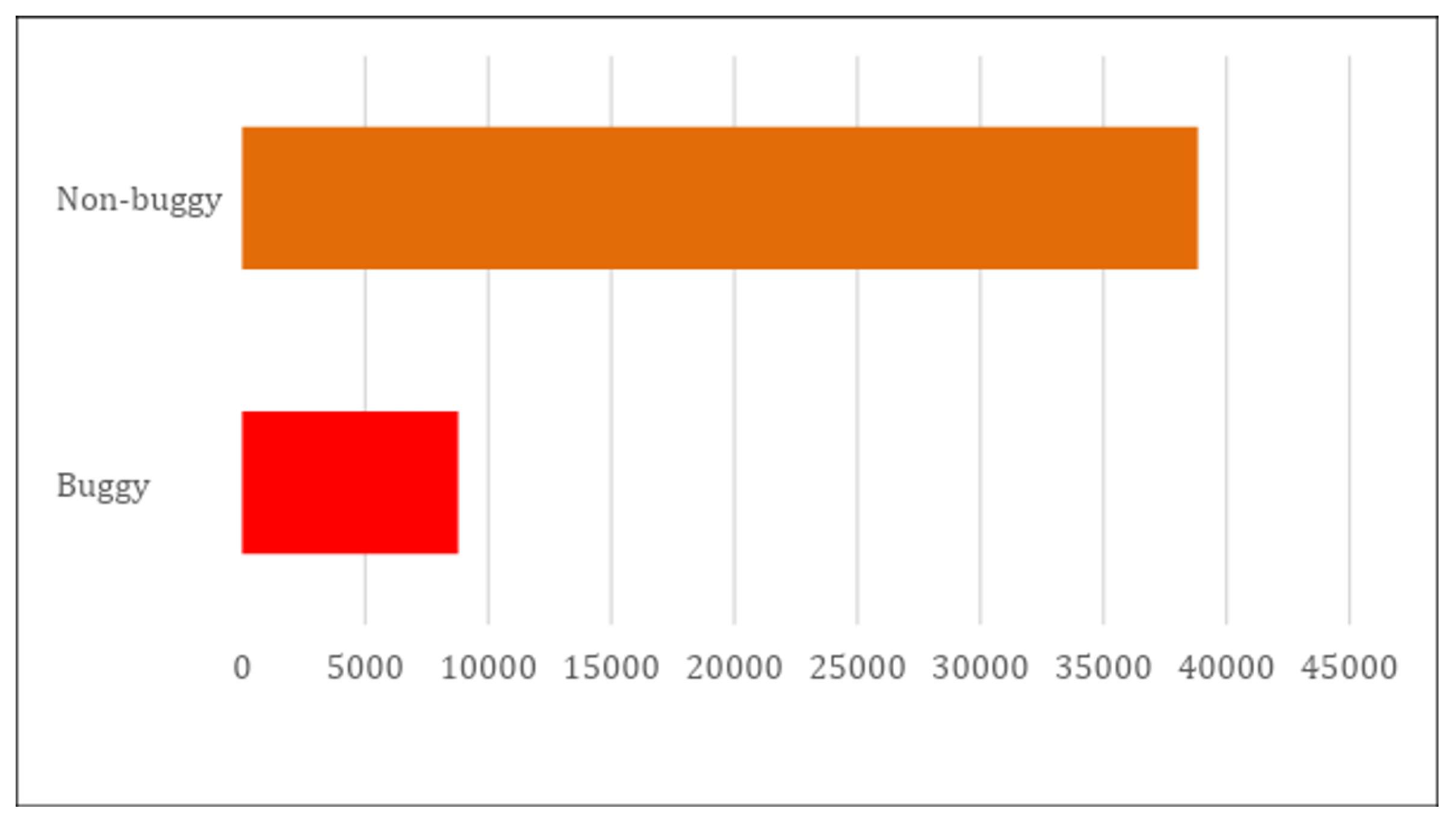
3.1. Dataset
3.2. Dataset Preprocessing
3.3. Machine Learning and Deep Learning Approaches
3.4. Evaluation
- (1)
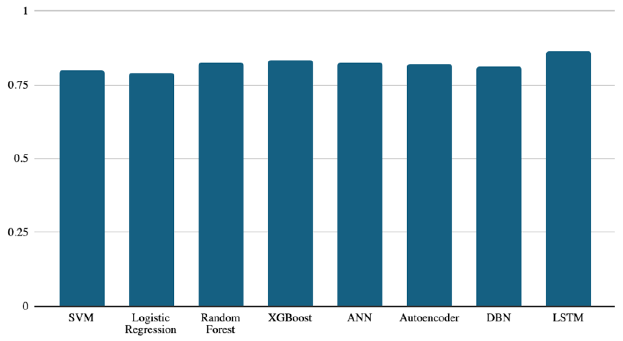
- Accuracy: Accuracy measures the proportion of predictions that are correctly classified (i.e., true positives and true negatives) by a model, ranging from 0 to 1, where a higher value means better model performance. Accuracy is computed based on the following formula:where = true positives, = true negatives, = false positives, and = false negatives.
- (2)
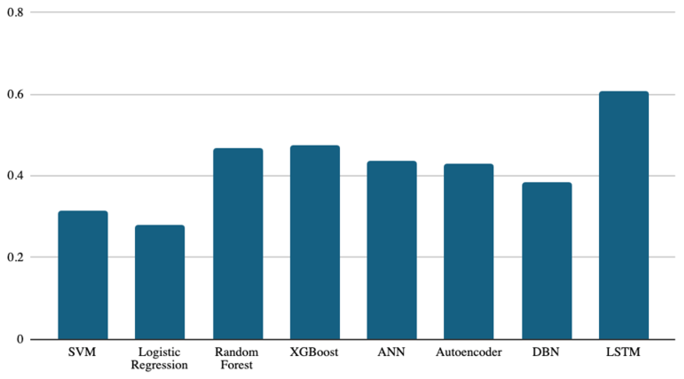
- Binary F1 Score: The binary F1 score is the harmonic mean of the precision and recall metrics, emphasizing the accuracy of positive predictions. It ranges from 0 to 1, where a large value indicates better performance. The following formula is used to calculate the binary F1 score:where the formulas for precision and recall are calculated as follows:
- (3)
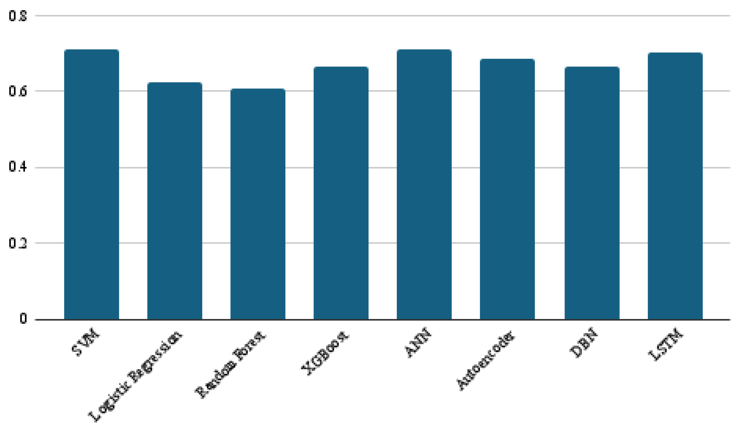
- Macro F1 Score: The macro F1 score is the average of the F1 scores for each class. It handles classes equally, regardless of each class’s support (i.e., the number of true instances). It is calculated using the following formula:where N is the number of classes (two classes in our case) and is the F1 score of class i.
- (4)
- Weighted F1 Score: The weighted F1 score is the weighted average of the F1 scores for each class. The average is weighted by the number of true instances in each class. The formula for the weighted F1 score is expressed as follows:where N is the number of classes, is the number of true instances for class i, and is the F1 score of class i.
4. Results and Discussions
5. Conclusions and Future Work
Author Contributions
Funding
Institutional Review Board Statement
Informed Consent Statement
Data Availability Statement
Acknowledgments
Conflicts of Interest
References
- Malhotra, R.; Chug, A. Software maintainability: Systematic literature review and current trends. Int. J. Softw. Eng. Knowl. Eng. 2016, 26, 1221–1253. [Google Scholar] [CrossRef]
- Huang, Q.; Shihab, E.; Xia, X.; Lo, D.; Li, S. Identifying self-admitted technical debt in open source projects using text mining. Empir. Softw. Eng. 2018, 23, 418–451. [Google Scholar] [CrossRef]
- Guo, J.; Yang, D.; Siegmund, N.; Apel, S.; Sarkar, A.; Valov, P.; Czarnecki, K.; Wasowski, A.; Yu, H. Data-efficient performance learning for configurable systems. Empir. Softw. Eng. 2018, 23, 1826–1867. [Google Scholar] [CrossRef]
- Boussaïd, I.; Siarry, P.; Ahmed-Nacer, M. A survey on search-based model-driven engineering. Autom. Softw. Eng. 2017, 24, 233–294. [Google Scholar] [CrossRef]
- Gondra, I. Applying machine learning to software fault-proneness prediction. J. Syst. Softw. 2008, 81, 186–195. [Google Scholar] [CrossRef]
- Iyer, S.; Konstas, I.; Cheung, A.; Zettlemoyer, L. Summarizing source code using a neural attention model. In Proceedings of the 54th Annual Meeting of the Association for Computational Linguistics 2016, Berlin, Germany, 7–12 August 2016; Association for Computational Linguistics: Kerrville, TX, USA, 2016; pp. 2073–2083. [Google Scholar]
- Mishra, S.; Sharma, A. Maintainability prediction of object oriented software by using adaptive network based fuzzy system technique. Int. J. Comput. Appl. 2015, 119, 24–27. [Google Scholar] [CrossRef]
- Ahmed, M.A.; Al-Jamimi, H.A. Machine learning approaches for predicting software maintainability: A fuzzy-based transparent model. IET Softw. 2013, 7, 317–326. [Google Scholar] [CrossRef]
- Mohd Adnan, M.; Sarkheyli, A.; Mohd Zain, A.; Haron, H. Fuzzy logic for modeling machining process: A review. Artif. Intell. Rev. 2015, 43, 345–379. [Google Scholar] [CrossRef]
- Chhabra, J.K. Improving package structure of object-oriented software using multi-objective optimization and weighted class connections. J. King Saud-Univ.-Comput. Inf. Sci. 2017, 29, 349–364. [Google Scholar]
- Elish, M.O.; Aljamaan, H.; Ahmad, I. Three empirical studies on predicting software maintainability using ensemble methods. Soft Comput. 2015, 19, 2511–2524. [Google Scholar] [CrossRef]
- Finlay, J.; Pears, R.; Connor, A.M. Data stream mining for predicting software build outcomes using source-code metrics. Inf. Softw. Technol. 2014, 56, 183–198. [Google Scholar] [CrossRef]
- Francese, R.; Risi, M.; Scanniello, G.; Tortora, G. Proposing and assessing a software visualization approach based on polymetric views. J. Vis. Lang. Comput. 2016, 34, 11–24. [Google Scholar] [CrossRef]
- Huo, X.; Li, M.; Zhou, Z.H. Learning unified features from natural and programming languages for locating buggy source code. In Proceedings of the IJCAI, New York, NY, USA, 9–15 July 2016; Volume 16, pp. 1606–1612. [Google Scholar]
- Haije, T.; Intelligentie, B.O.K.; Gavves, E.; Heuer, H. Automatic comment generation using a neural translation model. Inf. Softw. Technol. 2016, 55, 258–268. [Google Scholar]
- Ionescu, V.S.; Demian, H.; Czibula, I.G. Natural language processing and machine learning methods for software development effort estimation. Stud. Inform. Control 2017, 26, 219–228. [Google Scholar] [CrossRef]
- Jamshidi, P.; Siegmund, N.; Velez, M.; Kästner, C.; Patel, A.; Agarwal, Y. Transfer learning for performance modeling of configurable systems: An exploratory analysis. In Proceedings of the 2017 32nd IEEE/ACM International Conference on Automated Software Engineering (ASE), Urbana, IL, USA, 30 October–3 November 2017; pp. 497–508. [Google Scholar]
- Kaur, A.; Kaur, K. Statistical comparison of modelling methods for software maintainability prediction. Int. J. Softw. Eng. Knowl. Eng. 2013, 23, 743–774. [Google Scholar] [CrossRef]
- Li, L.; Feng, H.; Zhuang, W.; Meng, N.; Ryder, B. Cclearner: A deep learning-based clone detection approach. In Proceedings of the 2017 IEEE international conference on software maintenance and evolution (ICSME), Shanghai, China, 17–22 September 2017; pp. 249–260. [Google Scholar]
- Laradji, I.H.; Alshayeb, M.; Ghouti, L. Software defect prediction using ensemble learning on selected features. Inf. Softw. Technol. 2015, 58, 388–402. [Google Scholar] [CrossRef]
- Lin, M.J.; Yang, C.Z.; Lee, C.Y.; Chen, C.C. Enhancements for duplication detection in bug reports with manifold correlation features. J. Syst. Softw. 2016, 121, 223–233. [Google Scholar] [CrossRef]
- Luo, Q.; Nair, A.; Grechanik, M.; Poshyvanyk, D. Forepost: Finding performance problems automatically with feedback-directed learning software testing. Empir. Softw. Eng. 2017, 22, 6–56. [Google Scholar] [CrossRef]
- Menzies, T.; Greenwald, J.; Frank, A. Data mining static code attributes to learn defect predictors. IEEE Trans. Softw. Eng. 2006, 33, 2–13. [Google Scholar] [CrossRef]
- Malhotra, R.; Khanna, M. An exploratory study for software change prediction in object-oriented systems using hybridized techniques. Autom. Softw. Eng. 2017, 24, 673–717. [Google Scholar] [CrossRef]
- Malhotra, R. A systematic review of machine learning techniques for software fault prediction. Appl. Soft Comput. 2015, 27, 504–518. [Google Scholar] [CrossRef]
- Radjenović, D.; Heričko, M.; Torkar, R.; Živkovič, A. Software fault prediction metrics: A systematic literature review. Inf. Softw. Technol. 2013, 55, 1397–1418. [Google Scholar] [CrossRef]
- Rahimi, S.; Zargham, M. Vulnerability scrying method for software vulnerability discovery prediction without a vulnerability database. IEEE Trans. Reliab. 2013, 62, 395–407. [Google Scholar] [CrossRef]
- Tavakoli, H.R.; Borji, A.; Laaksonen, J.; Rahtu, E. Exploiting inter-image similarity and ensemble of extreme learners for fixation prediction using deep features. Neurocomputing 2017, 244, 10–18. [Google Scholar] [CrossRef]
- Yang, X.; Lo, D.; Xia, X.; Sun, J. TLEL: A two-layer ensemble learning approach for just-in-time defect prediction. Inf. Softw. Technol. 2017, 87, 206–220. [Google Scholar] [CrossRef]
- Ferenc, R.; Tóth, Z.; Ladányi, G.; Siket, I.; Gyimóthy, T. A public unified bug dataset for java and its assessment regarding metrics and bug prediction. Softw. Qual. J. 2020, 28, 1447–1506. [Google Scholar] [CrossRef]
- Jureczko, M.; Madeyski, L. Towards identifying software project clusters with regard to defect prediction. In Proceedings of the 6th International Conference on Predictive Models in Software Engineering, Timisoara, Romania, 12–13 September 2010; pp. 1–10. [Google Scholar]
- Zimmermann, T.; Premraj, R.; Zeller, A. Predicting defects for eclipse. In Proceedings of the Third International Workshop on Predictor Models in Software Engineering (PROMISE’07: ICSE Workshops 2007), Minneapolis, MN, USA, 20–26 May 2007; p. 9. [Google Scholar]
- D’Ambros, M.; Lanza, M.; Robbes, R. An extensive comparison of bug prediction approaches. In Proceedings of the 2010 7th IEEE Working Conference on Mining Software Repositories (MSR 2010), Cape Town, South Africa, 2–3 May 2010; pp. 31–41. [Google Scholar]
- Hall, T.; Zhang, M.; Bowes, D.; Sun, Y. Some code smells have a significant but small effect on faults. ACM Trans. Softw. Eng. Methodol. (TOSEM) 2014, 23, 1–39. [Google Scholar] [CrossRef]
- Tóth, Z.; Gyimesi, P.; Ferenc, R. A public bug database of github projects and its application in bug prediction. In Proceedings of the Computational Science and Its Applications—ICCSA 2016: 16th International Conference, Beijing, China, 4–7 July 2016; Proceedings, Part IV 16. Springer: Berlin, Heidelberg, Germany, 2016; pp. 625–638. [Google Scholar]
- Dong, X.; Liang, Y.; Miyamoto, S.; Yamaguchi, S. Ensemble learning based software defect prediction. J. Eng. Res. 2023, 11, 377–391. [Google Scholar] [CrossRef]
- Khleel, N.A.A.; Nehéz, K. Comprehensive study on machine learning techniques for software bug prediction. Int. J. Adv. Comput. Sci. Appl. 2021, 12, 8. [Google Scholar] [CrossRef]
- Ibrahim, A.M.; Abdelsalam, H.; Taj-Eddin, I.A. Software Defects Prediction At Method Level Using Ensemble Learning Techniques. Int. J. Intell. Comput. Inf. Sci. 2023, 23, 28–49. [Google Scholar] [CrossRef]
- Hammouri, A.; Hammad, M.; Alnabhan, M.; Alsarayrah, F. Software bug prediction using machine learning approach. Int. J. Adv. Comput. Sci. Appl. 2018, 9, 2. [Google Scholar] [CrossRef]
- Subbiah, U.; Ramachandran, M.; Mahmood, Z. Software engineering approach to bug prediction models using machine learning as a service (MLaaS). In Proceedings of the Icsoft 2018—Proceedings of the 13th International Conference on Software Technologies, Porto, Portugal, 26–28 July 2018; pp. 879–887. [Google Scholar]
- Khalid, A.; Badshah, G.; Ayub, N.; Shiraz, M.; Ghouse, M. Software defect prediction analysis using machine learning techniques. Sustainability 2023, 15, 5517. [Google Scholar] [CrossRef]
- Alzahrani, M. Using Machine Learning Techniques to Predict Bugs in Classes: An Empirical Study. Int. J. Adv. Comput. Sci. Appl. 2022, 13. [Google Scholar] [CrossRef]
- Marçal, I.; Garcia, R.E. Bug Prediction Models: Seeking the most efficient. 2024. preprint. Available online: https://www.researchsquare.com/article/rs-3900175/v1 (accessed on 20 September 2024).
- Jha, S.; Kumar, R.; Abdel-Basset, M.; Priyadarshini, I.; Sharma, R.; Long, H.V. Deep learning approach for software maintainability metrics prediction. IEEE Access 2019, 7, 61840–61855. [Google Scholar] [CrossRef]
- Yu, T.Y.; Huang, C.Y.; Fang, N.C. Use of deep learning model with attention mechanism for software fault prediction. In Proceedings of the 2021 8th International Conference on Dependable Systems and Their Applications (DSA), Yinchuan, China, 11–12 September 2021; pp. 161–171. [Google Scholar]
- Qiao, L.; Li, X.; Umer, Q.; Guo, P. Deep learning based software defect prediction. Neurocomputing 2020, 385, 100–110. [Google Scholar] [CrossRef]
- Alghanim, F.; Azzeh, M.; El-Hassan, A.; Qattous, H. Software defect density prediction using deep learning. IEEE Access 2022, 10, 114629–114641. [Google Scholar] [CrossRef]
- Al Qasem, O.; Akour, M.; Alenezi, M. The influence of deep learning algorithms factors in software fault prediction. IEEE Access 2020, 8, 63945–63960. [Google Scholar] [CrossRef]
- Tatsunami, Y.; Taki, M. Sequencer: Deep lstm for image classification. Adv. Neural Inf. Process. Syst. 2022, 35, 38204–38217. [Google Scholar]
- Liu, Q.; Zhou, F.; Hang, R.; Yuan, X. Bidirectional-convolutional LSTM based spectral-spatial feature learning for hyperspectral image classification. Remote Sens. 2017, 9, 1330. [Google Scholar] [CrossRef]
- Teshima, Y.; Watanobe, Y. Bug detection based on lstm networks and solution codes. In Proceedings of the 2018 IEEE International Conference on Systems, Man, and Cybernetics (SMC), Miyazaki, Japan, 7–10 October 2018; pp. 3541–3546. [Google Scholar]


| Type | Name | Path | … | WMC | CBO | … | LOC | Bug |
|---|---|---|---|---|---|---|---|---|
| Class | JavaConventions | … | … | 80 | 17 | … | 771 | 1 |
| Class | JavaCore | … | … | 301 | 58 | … | 4734 | 4 |
| Class | JavaModelException | … | … | 16 | 2 | … | 141 | 0 |
| Class | NamingConventions | … | … | 56 | 7 | … | 720 | 2 |
| Class | Signature | … | … | 428 | 4 | … | 2648 | 1 |
| Class | ToolFactory | … | … | 42 | 27 | … | 442 | 0 |
| Class | WorkingCopyOwner | … | … | 5 | 14 | … | 155 | 0 |
| Class | BuildContext | … | … | 20 | 3 | … | 114 | 0 |
| Class | CategorizedProblem | … | … | 4 | 3 | … | 93 | 0 |
| Class | CharOperation | … | … | 409 | 1 | … | 3645 | 0 |
| Class | CompilationParticipant | … | … | 8 | 3 | … | 109 | 1 |
| Approach | Key Hyperparameters |
|---|---|
| SVM | C = 1.0, kernel = rbf, gamma = scale |
| Logistic Regression | penalty = l2, C = 1.0, solver = lbfgs, max_iter = 1000 |
| Random Forest | n_estimators = 100, max_depth = none, min_samples_split = 2, min_samples_leaf = 1, max_features = auto |
| XGBoost | n_estimators = 100, learning_rate = 0.3, max_depth = 6, subsample = 1.0, colsample_bytree = 1.0, gamma = 0 |
| ANN | number of layers = 4 (layer 1: dense layer with 128 neurons; layer 2: dense layer with 64 neurons; layer 3: dense layer with 32 neurons; and layer 4: dense layer with 1 neuron (output layer)), activation functions = ‘relu’ for hidden layers and ‘sigmoid’ for output layer, batch normalization and dropout rate of 0.2 applied after each hidden layer, learning rate = 0.001, optimizer = Adam, loss = binary_crossentropy, epochs = 300, batch_size = 64, early stopping callback with monitor of ‘val_loss’ and patience of 5 |
| Autoencoder | Hyperparameters of the autoencoder: number of layers (excluding the input and output layers) = 5 (layer 1: dense layer with 256 neurons; layer 2: dense layer with 128 neurons; layer 3: dense layer with 60 neurons; layer 4: dense layer with 128 neurons; and layer 5: dense layer with 256 neurons), activation functions = ‘relu’ for hidden layers and ‘linear’ for output layer, learning rate = 0.001, optimizer = Adam, loss = mean_squared_error, epochs = 200, batch_size = 64, early stopping callback with monitor of ‘loss’ and patience of 10 Hyperparameters of the classifier: number of layers = 3 (layer 1: dense layer with 64 neurons; layer 2: dense layer with 32 neurons; layer 3: dense layer with 1 neuron (output layer)), activation functions = ‘relu’ for hidden layers and ‘sigmoid’ for output layer, dropout rate of 0.2 applied after each hidden layer, learning rate = 0.001, optimizer = Adam, loss = binary_crossentropy, epochs = 300, batch_size = 64, early stopping callback with monitor of ‘val_loss’ and patience of 5 |
| DBN | number of layers = 4 (layer 1: rbm layer with 128 neurons; layer 2: rbm layer with 64 neurons; layer 3: rbm layer with 32 neurons; layer 4: dense layer with 1 neuron (output layer)), activation functions = ‘sigmoid’ for output layer, learning rate = 0.001, optimizer = Adam, loss = binary_crossentropy, epochs = 100, batch_size = 64, early stopping callback with monitor of ‘val_loss’ and patience of 5 |
| LSTM | number of layers = 3 (layer 1: LSTM layer with 64 units; layer 2: LSTM layer with 32 units; layer 3: dense layer with 1 neuron (output layer)), activation functions = ‘sigmoid’ for output layer, dropout rate of 0.2 applied after each LSTM layer, learning rate = 0.001, optimizer = Adam, loss = binary_crossentropy, epochs = 100, batch_size = 64, early stopping callback with monitor of ‘val_loss’ and patience of 3, sequence length = 20 |
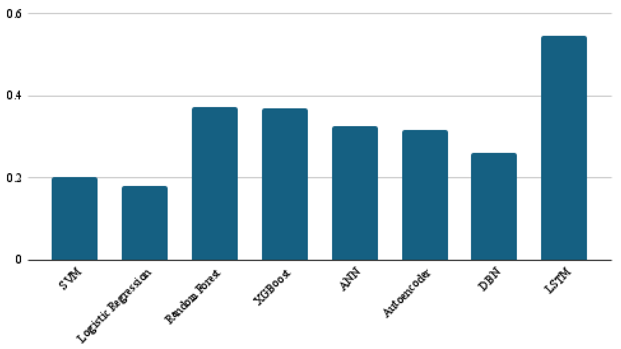
| Model | Accuracy | Macro F1 Score | Weighted F1 Score | Binary F1 Score |
|---|---|---|---|---|
| SVM | 0.84 | 0.61 | 0.80 | 0.31 |
| Logistic Regression | 0.83 | 0.59 | 0.79 | 0.28 |
| Random Forest | 0.84 | 0.69 | 0.83 | 0.47 |
| XGBoost | 0.85 | 0.69 | 0.83 | 0.47 |
| ANN | 0.85 | 0.68 | 0.83 | 0.44 |
| Autoencoder | 0.85 | 0.67 | 0.82 | 0.43 |
| DBN | 0.84 | 0.65 | 0.81 | 0.38 |
| LSTM | 0.87 | 0.77 | 0.87 | 0.61 |
Disclaimer/Publisher’s Note: The statements, opinions and data contained in all publications are solely those of the individual author(s) and contributor(s) and not of MDPI and/or the editor(s). MDPI and/or the editor(s) disclaim responsibility for any injury to people or property resulting from any ideas, methods, instructions or products referred to in the content. |
© 2024 by the authors. Licensee MDPI, Basel, Switzerland. This article is an open access article distributed under the terms and conditions of the Creative Commons Attribution (CC BY) license (https://creativecommons.org/licenses/by/4.0/).
Share and Cite
Albattah, W.; Alzahrani, M. Software Defect Prediction Based on Machine Learning and Deep Learning Techniques: An Empirical Approach. AI 2024, 5, 1743-1758. https://doi.org/10.3390/ai5040086
Albattah W, Alzahrani M. Software Defect Prediction Based on Machine Learning and Deep Learning Techniques: An Empirical Approach. AI. 2024; 5(4):1743-1758. https://doi.org/10.3390/ai5040086
Chicago/Turabian StyleAlbattah, Waleed, and Musaad Alzahrani. 2024. "Software Defect Prediction Based on Machine Learning and Deep Learning Techniques: An Empirical Approach" AI 5, no. 4: 1743-1758. https://doi.org/10.3390/ai5040086
APA StyleAlbattah, W., & Alzahrani, M. (2024). Software Defect Prediction Based on Machine Learning and Deep Learning Techniques: An Empirical Approach. AI, 5(4), 1743-1758. https://doi.org/10.3390/ai5040086