FedBirdAg: A Low-Energy Federated Learning Platform for Bird Detection with Wireless Smart Cameras in Agriculture 4.0

Abstract

Birds can cause substantial damage to crops, directly affecting farmers’ productivity and profitability. As a result, detecting bird presence in crop fields is crucial for effective crop management. Traditional agricultural practices have used various tools and techniques to deter pest birds, while digital agriculture has advanced these efforts through Internet of Things (IoT) and artificial intelligence (AI) technologies. With recent advancements in hardware and processing chips, connected devices can now utilize deep convolutional neural networks (CNNs) for on-field image classification. However, training these models can be energy-intensive, especially when large amounts of data, such as images, need to be transmitted for centralized model training. Federated learning (FL) offers a solution by enabling local training on edge devices, reducing data transmission costs and energy demands while also preserving data privacy and achieving shared model knowledge across connected devices. This paper proposes a low-energy federated learning framework for a compact smart camera network designed to perform simple image classification for bird detection in crop fields. The results demonstrate that this decentralized approach achieves performance comparable to a centrally trained model while consuming at least 8 times less energy. Further efficiency improvements, with a minimal tradeoff in performance reduction, are explored through early stopping.

1. Introduction

Digital agriculture, also known as Agriculture 4.0, represents the latest evolution in agricultural practices, integrating advanced technologies and tools to develop sustainable agricultural systems able to address food security challenges posed by a rapidly growing global population [1]. This new era of agriculture leverages the latest digital technologies, particularly artificial intelligence (AI) [2,3], robotics [2,4], and the Internet of Things (IoT) [5], among others. These technologies rely on advanced, complexity-optimized software and lightweight, cutting-edge hardware to meet the performance demands of agricultural applications. Since digital agriculture devices must operate outdoors for extended periods, energy efficiency is essential for maintaining reliable and effective systems.

Numerous studies have focused on enhancing energy efficiency by reducing power consumption in energy-constrained connected devices such as wireless sensor networks (WSNs) when utilized in agricultural applications [6], with a focus on wireless transmission, which represents the most significant component of energy costs in WSNs [7]. These studies provided energy-aware networking techniques and protocols to reduce this cost [6,8,9].

As edge devices become increasingly capable of handling complex computations, autonomous things (AuTs), and largely the Internet of Autonomous Things (IoAT), are gaining traction in many fields [10], enabling enhanced decision-making by providing “in-situ” localized knowledge. These innovative systems deploy AI models directly in the field, enabling real-time decision-making and bringing the concept of Edge AI to life [11]. However, the deployment of autonomous things tends to increase power consumption due to the computational intensity of these models. Moreover, building effective knowledge models requires a training phase that can be energy-intensive, as large datasets often involve substantial computations and classically need to be transmitted to a remote server for AI model development before the model weights are sent back to edge devices for on-site inference.

Edge training enables the development of localized knowledge without requiring large data transfers to a remote server, thereby conserving energy by reducing transmission costs. However, training on edge devices poses challenges, as it demands substantial computational power and memory [12], which are often difficult to provide on these devices due to their limited processing and storage capacities. Also, training a network of connected things can cause communication traffic congestion due to increased interactions between the nodes [13]. From an energy perspective, training an AI model directly on the edge for subsequent on-device inference offers practical advantages, particularly in reducing energy costs associated with data transmission. However, this approach demands greater computational power in edge devices during the training phase. To optimize energy efficiency, a balance must be achieved between the computational costs of on-edge training and the transmission savings it provides.

Introduced by Google in 2016 [14], federated learning (FL) is a distributed learning paradigm for edge training, where a model is deployed across multiple devices to train locally on their data and share their knowledge with each other [15]. After being initialized in every node, local model weights are iteratively trained on local data, aggregated into a global model, and re-deployed for further local, on-device training until convergence is achieved (Figure 1). As the Figure depicts, Step 0 is performed only once, before the federated learning loop starts, while steps 1–3 are repeated in each federated round, which creates the federated learning loop. Federated rounds continue until the model converges, meaning local training no longer improves the global model. Images of a pigeon and a crow illustrating steps 2 and 3 exemplify non-independently and identically distributed (non-IID) data, as a camera may capture data with only specific features (e.g., only pigeons or only crows) during model training yet encounter previously unseen features during post-deployment inference (e.g., both pigeons and crows).

Training a wireless smart camera network (WSCN) using an FL training scheme enhances decision-making accuracy uniformly across the network’s devices by enabling knowledge sharing among them. In cases where data is heterogeneous (IID) or non-IID, the local models address this issue through the global model aggregation process in FL. In other words, each camera learns from the collective data insights of other cameras without directly sharing their data. However, non-IID data can impede the performance of federated learning, making convergence more challenging [16]. Studies have been conducted to address these challenges through data-driven techniques [17] or optimizations of the federated aggregation (also referred to as averaging) scheme [18].

In this paper, we propose an energy-efficient platform powered by a RaspBerry PI WSCN to detect bird presence in crop fields. The proposed system was designed for on-field training, guided by user supervision prior to deployment, and enabling adaptable and autonomous decision-making for optimizing agricultural profitability as an innovative technology in digital agriculture. Our work sets a primary objective of introducing an initial proof of concept of a low-energy platform for a lightweight smart camera network for bird detection in agricultural settings. The focus is to enhance the trade-off between energy efficiency of the post-deployment training phase and detection accuracy using FL through an on-field training simulation with a training dataset composed of real-world agricultural samples from a crop field vulnerable to pest bird attacks that was monitored from April 2021 to June 2021. We propose an FL framework for the on-site training of smart cameras, focusing on minimizing transmission energy costs while achieving equivalent model performance in inference compared to traditional remote training. Our approach strategically balances the computational energy required for edge-based training with the reduced energy demands for data transmission, creating a more efficient and adaptable system for field deployments. Our main contributions are as follows:

• We introduce an energy-aware metric to assess the operational efficiency of AuTs in agricultural applications.
• We develop a FL-based framework for the on-site training of a WSCN platform tailored for energy-efficient learning in the field. This framework is evaluated, using the introduced metric, against traditional centralized learning approaches in a bird detection use case for crop protection.
• By examining trade-offs between computational energy and transmission energy in complex scenarios with highly non-IID data, we aim to provide insights into optimizing energy use for autonomous agricultural devices.

The paper is organized as follows. In Section 2, we review related work on AI and IoT applications in agriculture, focusing on training efficiency and FL applications with their advantages. We establish the novelty of our research by implementing FL specifically for the bird detection use case, with an emphasis on edge training efficiency. Section 3 outlines the methodology for implementing and analyzing our FL framework for on-site training by proposing a custom metric to assess the framework’s efficiency. In Section 4, we implement this framework, assessing its efficiency through the previously introduced metric. Section 5 presents the results and compares our framework’s efficiency to that of traditional centralized training methods. Section 6 provides conclusions on our findings, with insights into potential future work to enhance energy efficiency in edge AI, with a focus on optimizing inference-phase efficiency.

2. Related Work

Among the technologies driving digital agriculture, AI and IoT stand out as powerful tools for optimizing decision-making processes in farming. In training intelligent devices, FL, as previously introduced, offers several advantages, including enhanced privacy, energy efficiency, and knowledge sharing between trained devices. In this section, we review studies that integrate AI and IoT (or AIoT) applications in agriculture, emphasizing the applications and benefits of FL in the training phase of AIoT devices.

AI has found numerous applications in agriculture, whether integrated with computer vision for tasks like classification [19] or used for time-series forecasting [20]. Several platforms have developed AI-based automated decision-making systems to enhance agricultural efficiency and insight [21]. Additionally, the IoT has enabled the widespread use of connected devices to collect and process data directly at its source, allowing for more efficient and powerful agricultural systems [22]. Many agricultural use cases have harnessed AI and IoT technologies under the AIoT paradigm to boost performance and efficiency [23], utilizing FL, among other approaches, to train AuTs [24].

The application of AI and IoT in agriculture has become widespread and transformative, driving significant gains in efficiency and productivity across a range of agricultural use cases:

• Crop monitoring: IoT devices gather extensive data directly from the field, such as temperature, humidity, and soil moisture levels. AI models process this time-series data to predict crop growth and yield, enabling more informed decision-making for farmers [25,26,27,28].
• Disease detection: IoT-enabled cameras capture images of crops, which are analyzed via AI models using image recognition/classification techniques to identify symptoms of diseases early on. This allows for timely interventions, reducing the spread of diseases and improving crop health [29,30,31,32,33].
• Soil conservation: IoT sensors monitor key soil attributes like pH, nutrient levels, and moisture. AI algorithms analyze these data to provide recommendations for soil amendments and practices that enhance soil health and fertility [34,35].
• Water conservation: By tracking soil moisture and weather conditions, IoT devices feed data into AI systems that optimize irrigation schedules. This minimizes water usage while maintaining adequate hydration for crops, leading to better water conservation and reduced waste [36].
• Smart harvesting: IoT sensors continuously track environmental factors, providing real-time data that, when combined with AI models trained on historical datasets, can accurately identify the optimal time for harvesting. This approach maximizes yield quality while minimizing the risk of premature or delayed harvesting [37,38,39].
• Animal monitoring: IoT sensors, such as wearable devices, can monitor animal behavior, collecting data that track changes in key parameters indicative of health issues or other relevant conditions in livestock. These data, often represented as time series, can be used to train AI models capable of predicting diseases or classifying specific behaviors, enabling early intervention and improved herd management [40,41].
• Supply chain management: IoT devices monitor agricultural products throughout the supply chain, collecting data on conditions during transport and storage. AI analyzes this information to optimize logistics, manage inventory effectively, and reduce spoilage, ensuring that high-quality produce reaches consumers [42,43].

Overall, the integration of AI and IoT into agriculture is enabling smarter, data-driven practices, leading to improved sustainability, resource efficiency, and increased productivity.

In our study, we addressed the use case of detecting pest birds in crop fields using AI and IoT technologies. From an agricultural perspective, AIoT-enabled automated bird detection system can significantly enhance crop protection. Pest birds can cause extensive damage by eating seeds, fruits, or grains and spreading diseases. Detecting bird presence in real time helps prevent crop losses. Technically, detecting birds in a crop field is analogous to pest detection within the broader category of “disease detection” outlined above, as it also relies on image processing and classification techniques from camera-sensed data. The smart cameras capture field images, and AI models analyze these to identify distinct visual features indicative of birds, enabling timely interventions to protect crops.

Previous studies have focused on bird counting [44,45], species identification [46], or general bird recognition [47,48,49,50]. However, aside from [48], none of these works have specifically addressed the unique challenges of agriculture, such as detecting pest birds that pose a threat to crops. Moreover, they have not been trained on agricultural field images containing the specific pest bird species responsible for crop damage. Additionally, they do not consider the energy efficiency of the training process, a critical factor when deploying models on resource-constrained edge devices in agricultural environments, which is also lacking in the work of [48].

Unlike the works cited in this section on agricultural AI applications and bird detection, our goal is not to propose the most effective model in detecting pest birds accurately. Instead, we address the challenge of bird detection in agricultural crop fields through FL, with a strong emphasis on energy efficiency. Our approach prioritizes minimizing energy consumption during training, as our platform is designed to train directly in the field and quickly become functional for inference, reducing the energy demands of the training process. This work presents a simulation-based proof of concept, serving as a foundation for future on-field experiments with a platform of smart cameras capable of training efficiently in the field while maintaining reasonable inference performance. The study explores potential trade-offs between inference accuracy and the energy cost of training, which we aim to minimize using FL for initial convergence, followed by our proposed early stopping mechanism, LEFL.

Since its emergence, FL has been applied across various domains to train edge devices within the AIoT paradigm. Smart healthcare [51], smart industries [52], smart cities [53], and smart agriculture [54] are a few examples of domains that have already implemented FL frameworks to train their devices. The advantages of FL in these areas vary and include scalability, lower latency, data privacy, and energy efficiency, using fog aggregation to reduce frequent communication with a central server [55]. Also, FL offers significant advantages in environments with rapidly changing data, as training occurs directly at the edge, close to the data source [56]. This proximity allows the model to quickly adapt to new patterns and variations in real time, enhancing responsiveness and reducing latency compared to centralized training methods.

In our work, we explore the energy-efficiency advantage of FL in training agricultural connected devices, implementing a low-energy FL framework to train a MobileNet, a light convolutional neural network (CNN), in a WSCN for bird detection. Similar studies addressed the use of FL to train constrained devices in digital agriculture [54]. Recent studies highlighted several key advantages of applying FL in agriculture, such as data privacy and sovereignty [26,30,31,32,41,43,57,58], fault tolerance [32], reducing communication overhead [31], and improving model performance [28,33,59]. However, none of the surveyed works addressed the bird detection use case. Moreover, they did not place a primary emphasis on the energy efficiency of training agricultural AIoT devices.

Table 1. Previous works on FL applications in agricultural AIoT systems.

Paper	Use Case	IoT Device(s)/ Dataset(s)	AI Model(s)	FL Improvement(s)
[31]	Disease detection	UAVs	EfficientNet-B3	Communication overhead, data privacy
[32]	Weed detection	Hyperspectral Camera	Custom CNN	Fault tolerance, data sovereignty
[43]	Supply chain data management	Remote sensors, weather and soil data	Custom CNN, LSTM RNN	Data privacy
[26]	Crop yield prediction	Sensors, Cameras	ResNet-16, ResNet-28	Data privacy, data sovereignty
[30]	Maize leaf disease prediction	Cameras	AlexNet, SqueezeNet, ResNet-18, VGG-11, ShuffleNet	Data privacy
[57]	Intrusion detection	ToN-IoT dataset	GRU RNN	Data privacy
[41]	Automated animal activity recognition	Wearable sensors	CMI-Net	Data privacy
[58]	Securing agricultural IoT infrastructures	CSE-CIC-IDS2018, MQTTset, and InSDN datasets	Custom DNN, CNN, and RNN	Data privacy
[59]	Improving agricultural production	Smart sensors	Custom ML algorithm	Sensor control and adaptability
[28]	Crop classification	Climatic features	Gaussian Naive Bayes	Model accuracy
[33]	Disease and pest detection	Apple orchard images	ResNet-101	Model training speed
Our work	Bird detection	Smart cameras	MobileNetV2	Energy efficiency, knowledge sharing

provides an overview of recent research papers on FL applied to agricultural AIoT systems, specifying the use case, the used IoT device(s), the AI model employed, and the key benefit gained from implementing FL.

3. Methodology

We present LEFL, a novel low-energy FL framework for the efficient training of a WSCN to detect bird presence in crop fields. The efficiency of a connected device can be measured as its performance relative to energy consumption. While device performance can vary, depending on the application, we focus on the quality of information (QoI) provided. By contrast to QoI used for basic IoT devices that cannot learn or adapt, such as wireless sensor networks (WSNs) [60], we define quality of knowledge (QoK) as the enhanced QoI for more advanced IoAT devices, such as WSCNs, capable of learning through local model training and developing knowledge. We use model accuracy—either of the locally trained models or the global shared model—as the primary metric to evaluate the QoK of the WSCN. Achieving higher efficiency with LEFL involves achieving high QoK, reflected in accuracy enhancement by training the model while reducing the energy cost required for training through FL.

3.1. QoSAuT: Quality of Service of an Autonomous Thing

We introduce QoSAuT (quality of service of an autonomous thing) as an efficiency metric tailored for our use case. It is defined as the ratio of the shared model’s accuracy to the energy expenditure incurred during the training process. This metric captures the balance between model performance in terms of QoK and the energy costs required to achieve that level of QoK, providing a holistic measure of the device’s training efficiency. The metric can be expressed simply as follows:

$$QoSAuT(k,n_k,s_k)={\displaystyle \frac{\alpha .\Delta a_k}{n_k.(c{t}_k+{\mu }_k.s_k.x_k)+c{i}_k}}$$

(1)

• k = AuT index.
• $QoSAu{T}_k$ = QoSAuT of the trained AuT k.
• $\Delta a_k$ = accuracy gained via the model in k from the training, evaluated on unseen test data.
• $n_k$ = number of training rounds of k.
• $x_k$ = number of data frames sent via k in one training round.
• $c{t}_k$ = computational cost * of one training round in k.
• $c{i}_k$ = computational cost * of inference by the trained model in k.
• ${\mu }_k$ = transmission cost * of 1 byte by k.
• $s_k$ = size (in bytes) of one data frame sent and/or received via k.
• $\alpha$ = the maximum portion of the battery capacity we are willing to allocate ** for training.

* The energy costs should be represented as a percentage of the total battery capacity of the smart camera during its operation, providing a clear metric for the device’s energy consumption relative to its available power and making the QoSAuT a metric dependent on the capacity of the power storage used.

** The maximum percentage of the battery capacity allocated to the training phase is determined by the requirements of the subsequent inference phase—the more energy we allocate to training, the less we allocate to inference—which varies, depending on the specific application and its inference phase’s requirements in terms of energy. Exceeding this limit during training can significantly impact QoSAuT, which is why this factor is incorporated into the formula.

It is important to note that the use of accuracy in evaluating QoSAuT is primarily intended to assess the overall quality of the training process, providing insight into the decision-making quality of the AuT independent of its specific use case. For a more adapted evaluation of decision-making quality emphasizing the user perspective, particularly in the context of bird detection, recall would be more appropriate, as false negatives are more detrimental than false positives (false negatives lead to crop damage, while false positives result in unnecessary alerts). However, in our work, accuracy serves as a general metric for assessing the training quality and energy-cost tradeoff of the trained AuT, irrespective of the deployment task.

Based on the definition of the QoSAuT metric above, we can interpret the quality of the autonomous thing’s service by analyzing the quantitative metric’s value. These interpretations are summarized in

Table 2. Interpretation of the QoSAuT value.

QoSAuT	Quality of Service	Interpretation
$QoSAuT>1$	Good	The AuT learned at a relatively low energy cost.
$QoSAuT=1$	Average	The AuT learned near the limit of energy optimization.
$0<QoSAuT<1$	Bad	The AuT learned but at a relatively high energy cost.
$QoSAuT=0$	Very bad	The AuT did not learn.
$QoSAuT<0$	Disastrous	Theoretically impossible as the training must improve the model’s accuracy.

.

3.2. LEFL: A Low-Energy Federated Learning Framework

We leverage FL to aggregate locally trained models into a global model without exchanging the vast amounts of raw data typically required during the training phase. This approach is particularly beneficial for smart cameras, for which sharing image data would be bandwidth-intensive and impractical. Instead, FL transmits model weight updates, which are significantly smaller in size, reducing the communication load and enabling more energy-efficient, scalable training across the network’s nodes. While using FL for training helps alleviate network bottlenecks, allowing more data to be utilized effectively and improving the QoSAuT, our primary focus in this work is on the energy efficiency benefits, rather than the broader network-level advantages of FL. Federated learning (FL) can require numerous rounds for model convergence [14], and each round involves local computations on participating nodes. A high number of rounds can lead to increased energy consumption, presenting a challenge. Thus, a trade-off must be established between achieving model accuracy and minimizing energy costs. We propose LEFL, a low-energy federated learning framework that aims to address this by identifying the optimal point that balances consistent model accuracy with reduced energy expenditure. In our work, we leverage LEFL to improve the global QoSAuT of a WSCN.

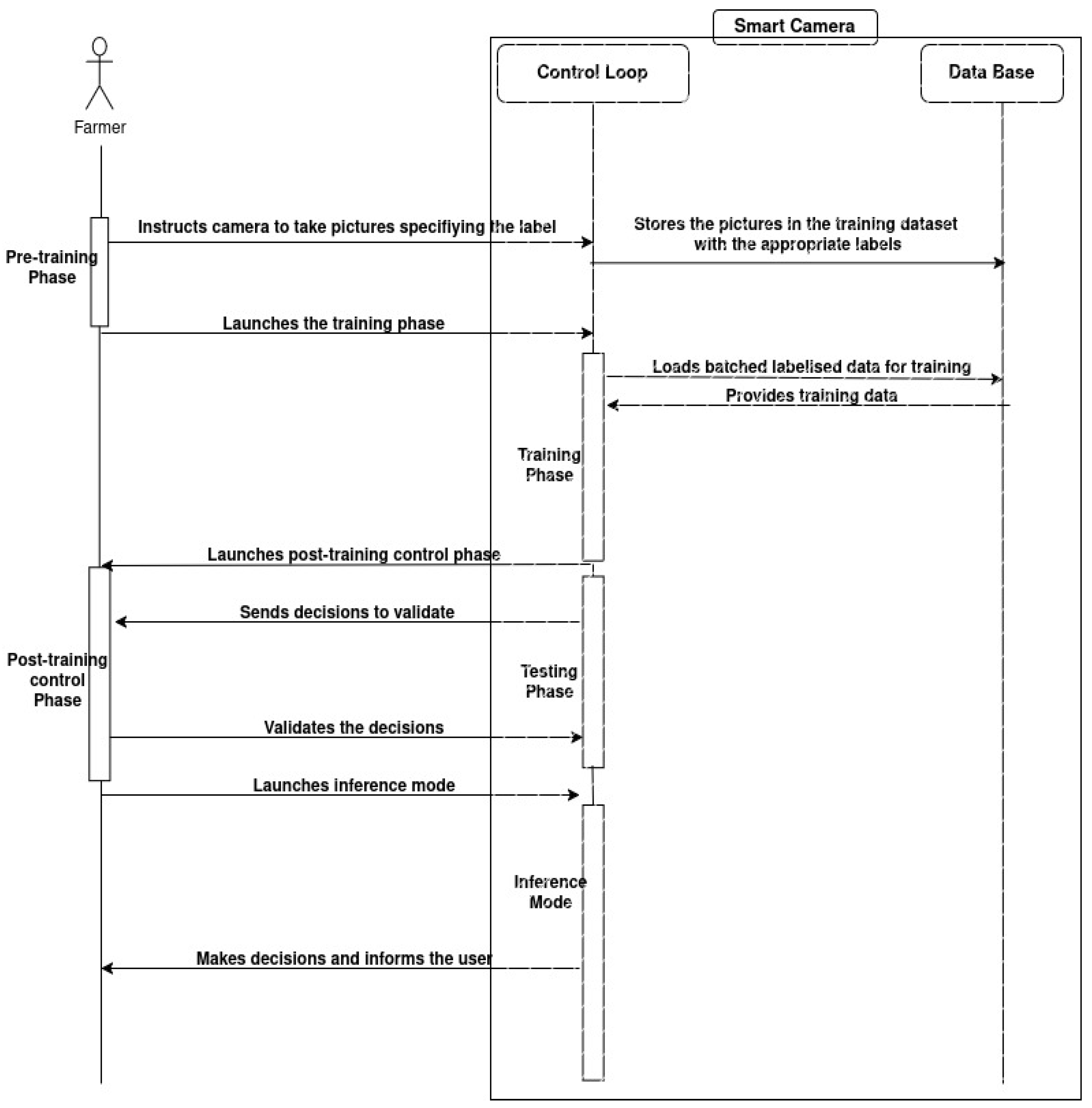
3.3. Bird Detection Scenario

To implement LEFL the framework, we consider a bird detection use case for crop field protection using a WSCN. The user deploys the cameras across separate fields and instructs them to capture an image whenever they see a bird. After gathering a sufficient number of images, the user initiates the learning process. Once the training is complete, the camera network begins autonomous detection. The user can periodically check the system’s performance and retrain the models if needed to improve autonomous decision-making.

Figure 2 presents the sequence diagram of the agricultural system to simulate. As shown in the Figure, the process begins with the farmer initiating a pre-training phase by instructing cameras to capture images of pest birds they detect in each camera’s related field. Once sufficient images are collected, the training phase commences. After training, a post-training control phase tests the model. If the farmer approves the results, inference mode begins; otherwise, the pre-training phase is restarted for further improvement. While in inference mode, the farmer can still intervene at any time by restarting the process if deemed necessary. It is important to note that, at no point during the system’s operation—whether before, during, or after training—does it transmit raw data to the user, only instructions/decisions that are lightweight messages. Keeping data entirely on the edge ensures enhanced privacy and minimizes transmission costs.

4. Implementation

Our work presents a straightforward simulation of the previously described agricultural system. The implementation models a simple scenario where a farmer manages two similar crop fields requiring protection from pest birds. The simulation considers two pest bird species—pigeons and crows—highlighting the system’s ability to detect different bird species to effectively safeguard the crops. To implement this simulation, we selected hardware likely to be optimal for powering a WSCN, prioritizing high computational capacity to handle the demanding processing tasks required for image classification (Section 4.1). Additionally, the training software and frameworks were carefully selected to optimize local training tasks, ensuring efficient and effective learning processes on edge devices (Section 5.3.1). Finally, we gathered a dataset closely resembling real-world conditions to train the system effectively, ensuring its applicability and reliability in practical scenarios (Section 4.3).

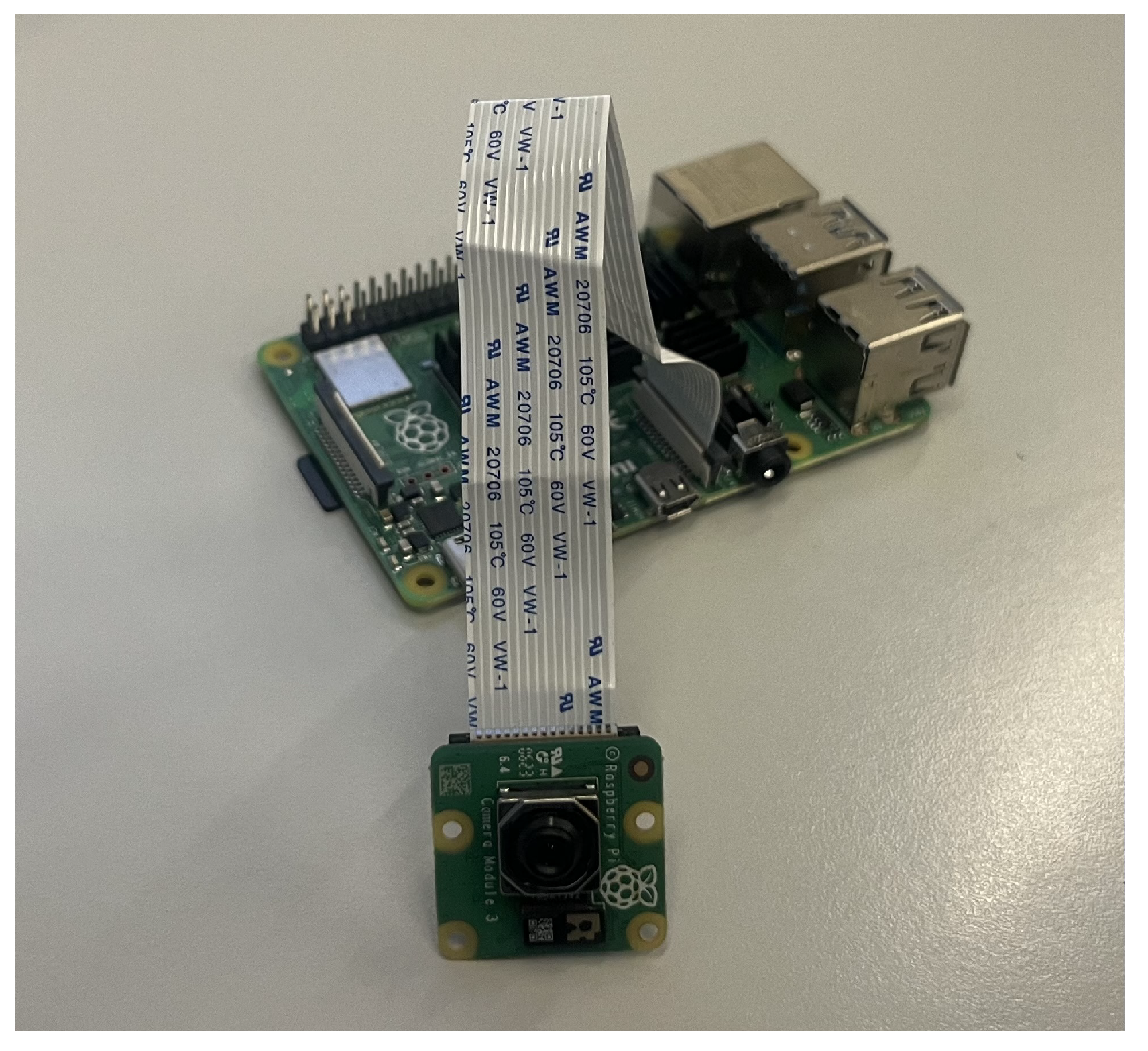
4.1. Hardware

We opted for RaspBerry Pi 4 (Sony UK Technology Centre, Pencoed, UK) as a hardware implementation that delivers high-performance inference, supports efficient network communication, and maintains cost-effectiveness.

Table 3. Comparative table of Raspberry Pi 4 and market competitors for local image classification and training.

Device	CPU	GPU/NPU	Memory	MobileNetV2 Performance (FPS)	Wireless Communication	Training Energy Cost (Power)	Price (USD)
Raspberry Pi 4	Quad-core Cortex-A72 @ 1.5 GHz	VideoCore VI GPU (32 GFLOPS)	1–8 GB LPDDR4	3–4	Wi-Fi 5 (802.11ac), Bluetooth 5.0	3.4 W	50
Jetson Nano	Quad-core Cortex-A57 @ 1.43 GHz	128 CUDA cores (1.8 TOPS)	4 GB LPDDR4	10–12	External USB Wi-Fi adapter required	5–10 W	99
Google Coral Dev Board	ARM Cortex-A53	Edge TPU (4 TOPS)	1 GB LPDDR4	50–60	Wi-Fi 5 (802.11ac), Bluetooth 4.1	2 W	129
Radxa Zero	Quad-core Cortex-A55 @ 1.4 GHz	Mali-G52 (0.6 TOPS NPU)	1–8 GB LPDDR4	2–3	Wi-Fi 5 (802.11ac) (only in advanced model), No wireless in basic model	3 W	40
BeagleBone AI	Dual-core Cortex-A15 @ 1.5 GHz	PowerVR SGX544 + C66x DSP	1 GB DDR3L	5–6	External USB Wi-Fi adapter required	7 W	120

offers a comparative overview of Raspberry Pi 4 against other market competitors designed for local image classification and training tasks. It highlights key specifications, including computational performance (focused on MobileNetV2), average training energy cost, price, and wireless communication capabilities with a focus on Wi-Fi compatibility.

Raspberry Pi 4 and the Radxa Zero stand out as the most accessible hardware options in terms of both affordability and energy efficiency, aligning well with the requirements of our system. Note that the Radxa Zero offers slightly lower performance compared to the Raspberry Pi 4 but demonstrates better energy efficiency. However, we excluded the Radxa Zero from consideration because our implementation requires hardware suitable for wireless communication, an important requirement for building a WSCN. Radxa Zero’s basic model lacks integrated Wi-Fi capabilities. Considering these factors, we selected Raspberry Pi 4 as the most suitable choice for our implementation.

We focused on Wi-Fi, as it is the simplest and most practical communication technology for implementing our WSCN; Wi-Fi networks are already established in many agricultural settings, eliminating the need for additional communication infrastructure.

The computing unit selected for the system is Raspberry Pi 4, while the data acquisition component is the Raspberry Pi Camera Module. The simulated smart camera system (RaspBerry PI 4 + camera) is shown in Figure 3.

4.2. Software

As mentioned earlier, we opted for MobileNetV2 as the base model to equip our wireless smart cameras with AI-based classification capabilities. It is a lightweight, efficient CNN chosen for its suitability in performing image classification [61], which is our primary task.

Table 4. Comparison of lightweight image classification models for edge devices.

Model	Top-1 Accuracy	Model Size	Latency (CPU)	Energy Consumption	Notable Strengths
MobileNetV2	71.8%	14 MB	20 ms	Moderate	Lightweight, efficient for edge devices.
EfficientNet-B0	77.1%	20 MB	24 ms	Moderate-High	Higher accuracy; more resource-demanding.
SqueezeNet	58.1%	4.8 MB	18 ms	Low	Extremely lightweight, lower accuracy.
ShuffleNet V2	69.4%	8 MB	22 ms	Low	Faster on mobile CPUs, good trade-off.

provides a comparative overview of our model alongside the most commonly used lightweight models for local edge image classification tasks. MobileNetV2 offers a strong balance between accuracy and computational efficiency, making it ideal for resource-constrained devices performing image classification.

To train our model, transfer learning was an effective technique, particularly in resource-constrained environments. This approach involves leveraging pre-trained models, which have already learned useful features on large datasets, such as ImageNet [62]. The model can be used in two ways: either without fine-tuning, with the pre-trained layers serving as feature extractors and leaving only the classification layers for adaptation to the new task, or with fine-tuning, with additional layers, beyond the classification ones, being updated to refine the model’s performance for the specific task at hand.

Our model was designed specifically for mobile and embedded vision applications, and it utilizes depthwise separable convolutions, reducing the model size and computational complexity without compromising accuracy [61]. Transfer learning further enhances this by reusing its robust feature extraction layers while training only the final classification layers. This modular adaptability aligns with the requirements of applications like bird detection, for which the aim is to efficiently classify images into categories on constrained hardware performing in a changing environment. Figure 4 shows the plot of the architecture flow of our MobileNetV2-based model. As shown in the figure, our model contains a Tensorflow Keras MobileNetV2 as a base model, plus a fully connected GlobalAveragePooling2D layer as a classification head. The classification head converts the MobileNetV2’s output features to a single 1280-element vector per image for further simplification to a scalar output (birds/no-birds) to be performed via the final dense layer. Note that, if fine-tuning is not used, only the weights of the classification head are updated during training. Otherwise, more layers of the “Functional” block are unfrozen for further training.

We trained our model using the TensorFlow framework. Developed by Google [63], TensorFlow is a popular framework for deep learning, known for its versatility and wide adoption in various edge devices, including Raspberry Pi. On its Lite version, it supports model training and inference on resource-constrained devices, making it suitable for edge AI applications.

Table 5. Comparative table of TensorFlow and PyTorch for edge training and deployment.

Feature	TensorFlow	PyTorch
Ease of Use	High-level API with extensive documentation	Dynamic computational graph, more flexible
Performance on edge devices	Optimized for edge deployment with TensorFlow Lite	Requires optimizations for edge deployment
Model deployment	Easy integration with TensorFlow Lite for mobile/edge	Model conversion needed for deployment
Resource efficiency	Highly optimized for low-resource devices	May require more resources for similar tasks

presents a comparison between TensorFlow 2.16 and PyTorch 2.4—another popular framework for deep learning (DL)—with a focus on their suitability for edge training and inference. It also highlights their resource efficiency, particularly in the context of power-constrained devices.

We deploy our WSCN devices with the model illustrated in Figure 4, ensuring a unified approach to local training. The base model (MobileNetV2) is pre-trained on ImageNet dataset. After the classification head is added, the base model is frozen and the head is trained on each local device’s data to develop a classification knowledge. To achieve global classification performance across all devices, we employed FL to facilitate global model convergence, ensuring that each device attains the same classification knowledge while preserving the uniqueness of local datasets.

Global model convergence in FL often requires numerous iterations [14], which can significantly impact energy consumption. Therefore, our focus is on optimizing the tradeoff between achieving a sufficient convergence rate and minimizing the number of iterations to conserve energy. This approach defines our low-energy FL framework, which we name LEFL, designed explicitly for energy-efficient training in resource-constrained environments like a WSCN.

To implement our FL framework, we leveraged ready-to-use functionalities provided via FL libraries. Among the available options, we selected Flower [64], a robust and versatile framework tailored to establishing a client–server architecture and managing FL strategies. Flower simplifies the development and deployment of FL systems with its lightweight and adaptable design.

Table 6. Comparative table of Flower and other FL frameworks for edge training efficiency.

Framework	Ease of Use	Communication Efficiency	Energy Efficiency	Edge Adaptability	Observations
Flower	High	Optimized	High	Excellent	Lightweight, flexible, and edge-focused, DL framework-agnostic
TensorFLow FL (TFF)	Moderate	Moderate	Moderate	Good	Focused on TensorFlow-based implementations
PySyft	Moderate	Good	Moderate	Moderate	Emphasizes security but less edge-specific
FedML	Moderate	Optimized	High	Good	Versatile but more complex for lightweight systems
LEAF	Low	Basic	Low	Limited	Designed primarily for academic purposes where performance is not the primary focus

provides a comparative overview of various FL libraries [65], highlighting Flower’s suitability for our specific requirements.

From the comparative table, it is evident that, while TFF aligns well with our choice of TensorFlow as a DL framework, its communication infrastructure does not prioritize wireless efficiency, which is crucial for our application. Flower, on the other hand, is designed with wireless communication efficiency in mind, making it more suitable for our system, which relies on wireless communication for federated training. While FedML offers optimized communication between devices during federated training, its adaptability to edge devices remains less refined compared to Flower. By leveraging Flower, we ensure an edge-optimized, scalable, communication-optimized, and energy-efficient implementation of our LEFL framework, which is essential for the resource-constrained devices in our WSCN.

The LEFL framework used in this work is a custom solution combining Flower for federated training and communication between devices and TensorFlow for efficient local model training on edge devices. This integration enables the collaborative training of a global model while maintaining energy efficiency.

The key contribution of our framework is an algorithm designed to determine the optimal stopping point for FL, an approach commonly referred to in the literature as an early stopping strategy. Resource-efficient early stopping strategies, like FLrce [66], ensure energy conservation without compromising model performance. In our work, unlike [66], where the stopping criterion was the number of conflicting clients, the stopping criterion of our strategy was guided by the $QoSAuT$ metric, defined in Section 3.1, which quantifies the trade-off between the trained model’s acquired performance (accuracy) during training and its associated energy cost. We defined the partial $QoSAuT$, $QoSAu{T}_i$, as the trade-off between the model’s acquired performance in one federated round, i, and its associated energy cost. Using $QoSAu{T}_i$, the algorithm dynamically evaluates the learning progress, halting the federated process when additional learning iterations yield diminishing returns in performance relative to energy expenditure. This adaptive strategy allows the LEFL framework to achieve both effective learning and operational sustainability through a novel energy-efficient early stopping strategy.

$QoSAu{T}_i$ is computed locally for each client and for each round. For instance, for the smart camera, k, in each round, i, we compute $C{r}_{i,k}$, the stopping criteria of k at the round i with the following formula:

$$C{r}_{i,k}=QoSAu{T}_i(k,1,8)={\displaystyle \frac{\alpha {\Delta }_i{a}_k}{c{t}_{i,k}+8{\mu }_k{x}_{i,k}+c{i}_k}}$$

(2)

We use, as fixed parameters, 1 as one training round (the federated round) and 8 = 4 × 2, as the size of a float is 4 bytes (transmitted model weights being floats), and 2 is the number of times a weight is sent across the network (sent from the client to the server and then from the server to the client after being updated).

And as variable parameters, we used the following:

• $\alpha$ = factor defined in Formula (1).
• ${\Delta }_i{a}_k$ = gained accuracy in the round, i, via the trained model in k.
• $x_{i,k}$ = number of weights sent in the round, i, via k.
• $c{t}_{i,k}$ = computational cost of the round, i, in k.
• $c{i}_k$ = inference cost of the model in k.
• ${\mu }_k$ = transmission cost of 1 byte via k.

Since the number of weights transmitted in a federated round and the cost of sending 1 byte via the device are invariant data during the training process, and the inference cost of the model, $c{i}_k,$ remains constant, regardless of the training process, the variant parameters of our early stopping strategy are as follows: $c{t}_{i,k}$ and ${\Delta }_i{a}_k$.

In each training round, we compute $c{t}_{i,k}$ directly, but computing ${\Delta }_i{a}_k$ requires the accuracy from the previous round. To address this, we maintain a global variable, $A\left[\right]$, which stores the achieved accuracy at the end of each round.

In FL, clients generally experience increasing accuracy during training. However, it may occasionally dip temporarily in a given round before resuming its upward trend. To address this, the early stopping mechanism is triggered if the $QoSAu{T}_i$ remains poor for two consecutive rounds, indicating a confirmed trend of declining training efficiency and justifying the need for early termination.

We implement the early stopping (ES) strategy of our LEFL framework based on the $QoSAu{T}_i$ values from the last two consecutive federated rounds. These values are calculated following Algorithm 1.

Algorithm 1 Computing $QoSAu{T}_i$.

Require:  round i, accuracies table $A\left[\right]$, factor $\alpha$, model’s number of weights x, the cost of transmitting 1 byte $\mu$, the cost of inference $ci$, the computational cost of the training round i$ct\left(i\right)$, as a percentage of the total available battery power. if $i=0$ then  return False end if $\Delta a\leftarrow A\left[i\right]-A[i-1]$ $Q\leftarrow {\displaystyle \frac{\alpha .\Delta a}{ct\left(i\right)+8.\mu .x+ci}}$ return Q

Our LEFL framework was designed to terminate federated learning rounds once the improvement in accuracy no longer justifies the corresponding energy expenditure, ensuring an optimal balance between performance—the accuracy of the model—gains and energy efficiency.

We conceptualized a function, FL(i), that performs the training for a federated round, i, updating the table with the accuracy achieved during the round. Specifically, FL(1) updates $A\left[0\right]$ with the initial accuracy before training and $A\left[1\right]$ with the model’s accuracy upon the first round’s completion. Additionally, we defined CT(i) as a function that computes the computational cost associated with the i-th federated round and CI() as a function to compute the computational cost of one inference via the model. Also, we assumed that the trained model had an attribute trainable_weights that returns the number of its trainable weights.

Using Algorithm 1 to compute $QoSAu{T}_i$, which we call “Q”, and the computational cost functions CT and CI, we implemented the LEFL ES as presented in Algorithm 2.

Algorithm 2 LEFL ES Algorithm.

Require:  factor $\alpha$, total available battery power $W_{max}$, the cost of transmitting 1 byte to the server M $\mu \leftarrow {\displaystyle \frac{M}{W_{max}}}$ $x\leftarrow model.trainable\_weights$ $ci\leftarrow {\displaystyle \frac{CI\left(\right)}{W_{max}}}$ $A\left[\right]\leftarrow \left[\right]$ $i\leftarrow 0$ $Cr\leftarrow \mathbf{False}$ while $Cr==$ False do  $i\leftarrow i+1$  if $FL(i,A[\left]\right)$ then   $ct\leftarrow {\displaystyle \frac{CT\left(i\right)}{W_{max}}}$   $Cr\leftarrow$$Q(i,A[],\alpha ,x,\mu ,ci,ct)<1$ && $Q(i-1,A[],\alpha ,x,\mu ,ci,ct)<1$  else   break  end if end while

Note that the LEFL’s Early Stop algorithm was implemented on the client side (i.e., executed on each device k). If the stopping criterion is not met, the while loop continues until the server terminates the FL process upon achieving global convergence, and then every device k stops training.

4.3. Data

4.3.1. Dataset Overview

We trained our MobileNetV2 model, distributed across two smart cameras, as designed in Section 4.1, using a dataset of images taken directly from a field of germinating crops or newly sown seeds, which are highly attractive to pest birds. This dataset was provided by Corentin Barbu from the Agronomie Unit of INRAE and Christophe Sausse from Terres Inovia [67].

We annotated the data with two labels: $birds$ (a pest bird species is present in the crop field) and $no\_birds$ (no pest bird species is present in the crop field). Two pest bird species are photographed on the monitored field: pigeons and crows. These species are particularly drawn to germinating crops and newly sown seeds, making them frequent targets for pest management strategies in agricultural environments.

The images were collected from a single plantation, with the field divided into two sections, each monitored via a separate camera, during a defined growth period (April to June) when grains attract pest birds. Due to seasonal constraints, the dataset does not include rainy or dusty conditions, which aligns with our objective of simulating on-field training during a consistent plantation growth period—where weather conditions typically remain stable throughout the training phase. The dataset includes bird samples captured at varying distances from the camera and at different times of the day (dawn, midday, and dusk), ensuring a balanced representation of lighting conditions. Additionally, it captures diverse bird sizes and behaviors, including birds flying close to the ground, resting on the soil, and appearing in various positions.

Figure 5 illustrates two samples from our dataset labeled as $birds$, showcasing the two pest bird species of our study: pigeons and crows. Typically, a sample from our dataset will feature both species, but one species can be more prominently represented in the crop field than the other.

4.3.2. Data Distribution for Training

After duplicates, outliers, and unusable images were removed during the data-cleaning process, we obtained a curated dataset ready for training containing 115 images (57 $birds$ + 58 $no\_birds$).

Since the dataset is balanced, containing an equal number of “$birds$” and “$no\_birds$” samples, accuracy is an appropriate metric for evaluating both training quality and overall model performance, eliminating the need for the F1 score.

To perform our training strategy, we split the dataset into two subsets: one for training (45 $birds$ + 47 $no\_birds$) and one for testing (12 $birds$ + 11 $no\_birds$). The training subset was then subdivided as follows: $75\%$ for training (34 $birds$ + 35 $no\_birds$) and $25\%$ for validation (11 $birds$ + 12 $no\_birds$).

Table 7. Data distribution of our training strategy.

Subset	$\mathbf{Birds}$	$\mathbf{No}\_\mathbf{Birds}$	All
Training ($60\%$)	34	35	69
Validation ($20\%$)	11	12	23
Testing ($20\%$)	12	11	23
Total ($100\%$)	57	58	115

provides an overview of the data distribution used in our training strategy.

Additionally, as a pre-processing step, we rescaled the images to 160 × 160 to match the input layer of our model to be trained (Figure 4). In real-world field deployment, the smart cameras capture images at an optimal resolution, providing 160 × 160-pixel images directly to the model for training. This approach significantly enhances energy efficiency by reducing both acquisition and computational costs, as it eliminates the need for additional preprocessing or resizing.

Given the small dataset size (115 samples), allocating 60% for training ensured that the model had enough examples to learn meaningful patterns while avoiding excessive overfitting. The 20% validation set is essential for tuning hyperparameters and preventing overfitting by evaluating model performance on unseen data during training. A validation set that is too small may lead to unstable results, while a larger one would reduce the already limited training set. With only 115 samples, more aggressive splits (e.g., 70/15/15 or 80/10/10) would either reduce validation robustness or limit the training set. The 60/20/20 split maintains a balance between learning, validation, and unbiased testing, which is particularly crucial in low-data scenarios.

As highlighted in Section 2, our addressed use case aligns closely with state-of-the-art pest and disease detection research. To contextualize the limitation of our dataset size,

Table 8. Dataset sizes of similar works (plant disease detection).

Paper	Dataset Size	Data Type
[29]	2029	Images
[30]	3852	Images
[31]	5400	Images
[32]	104,544	Hypervoxels
Our work	115	Images

presents a comparison of the sizes of the datasets employed in training classification models in similar studies, emphasizing the relative scale of data available for our training process.

However, in [31], 5400 samples were obtained from only 200 using data augmentation techniques, which included applying four different rotations and one mirroring transformation. In our work, we avoided using these techniques, as these augmentations could generate unrealistic or irrelevant data samples. Such transformations are not representative of real-world scenarios of a bird detection use case, given that our monitoring cameras remain fixed, capturing images consistently from the same angle of view. This fixed perspective makes it crucial to retain the natural orientation and positioning of elements within the captured scenes.

We mitigate our small dataset’s limitation by employing two key techniques: First, transfer learning (Section 5.3.1), as a pre-trained model on a broader dataset, enables the system to perform effectively even with a small training dataset by leveraging pre-existing knowledge. Second, the operational design of our system ensures adaptability to new data. Users can intervene to halt inference mode if significant changes in the data are detected and initiate additional training phases (Section 3.3), allowing the model to continuously adapt to real-world variations. Finally, our application use case differs from plant disease detection in that our images involve simpler scenarios, such as birds present in a field, whereas identifying diseases often involves subtle and complex visual patterns. This makes the need for a larger dataset less critical in our case, as the task is less intricate.

To visualize our training data (Training + Validation subsets) distribution in the feature space and the separability of the two classes ($birds$ and $no\_birds$), we plot its feature space visualization (FSV). After reducing the data dimensionality, with principal component analysis (PCA), to two dimensions (two principal components), we obtained the FSV of our training data, as presented in Figure 6. Note that the FSV is represented in two dimensions, using only the first two principal components (PCs). This dimensionality reduction leads to overlapping representations, which might obscure potential separability observable in the original high-dimensional space. The overlap can also be attributed to the input image size (160 × 160), where images labeled as $birds$ with relatively distant birds appear visually similar to images labeled as $no\_birds$, as the low resolution fails to capture sufficient features of the far-spotted birds. Furthermore, images labeled as $no\_birds$ tend to cluster more tightly, reflecting the uniformity of crop field images without intruders, whereas $birds$-labeled images are more sparsely distributed. This sparsity arises from the inclusion of two pest bird species, pigeons and crows, each introducing distinct feature sets.

4.3.3. Data Distribution over Clients

To highlight the performance of our LEFL-based platform, we evaluated its effectiveness in addressing the bird detection task using two wireless smart cameras under two distinct scenarios:

• During the training phase, both crop fields monitored via the cameras were equally likely to attract either bird species (homogeneous distribution). To replicate this scenario in our study, we split the training data between the two clients (cameras) in a balanced manner, ensuring an even representation of both bird species across the datasets. This data distribution over clients is called identically independent distribution (IID), meaning the data samples across all clients are independently drawn from the same probability distribution. ($S_1$).
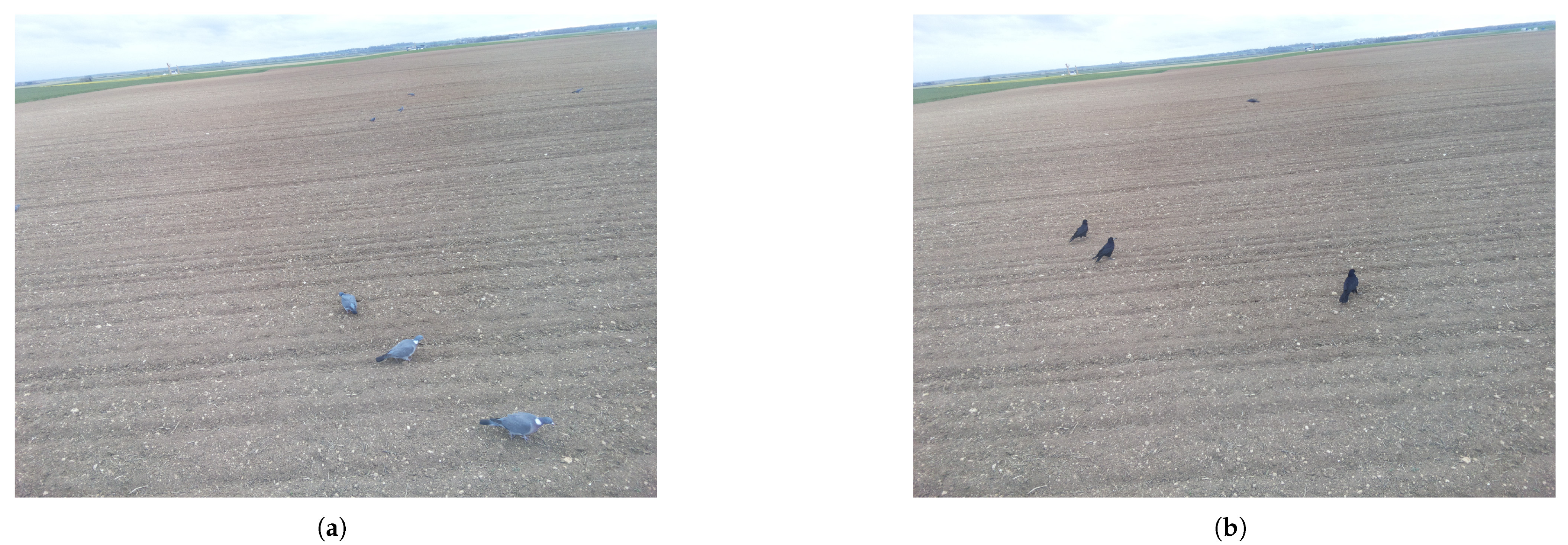
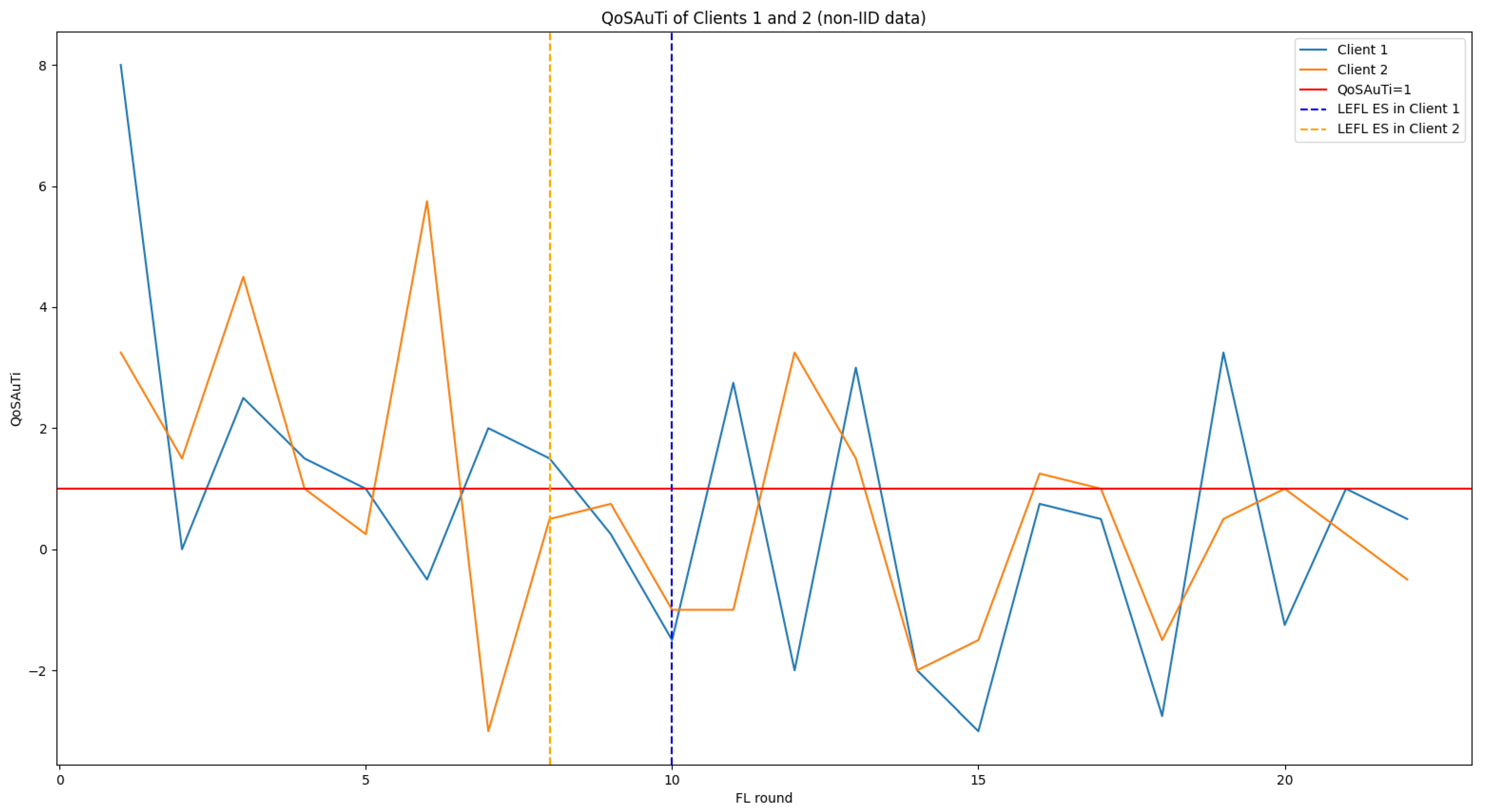
• During the training phase, one crop field is more likely to attract pigeons, while the other tends to attract crows. To simulate this scenario, we distribute the training data unequally between the two clients, assigning images showcasing more pigeons to the first client and images showcasing more crows to the second. This ensures a heterogeneous data distribution across the clients. Such a distribution is termed non-identically independent distribution (non-IID), indicating that data samples on each client are drawn from distinct probability distributions ($S_2$).

Our training dataset consists of 92 images, out of which 45 are labeled as $birds$. Among these, 26 images predominantly feature pigeons, while 19 images primarily contain crows.

In both scenarios, we split the training set (comprising the training and validation subsets) across the clients while keeping the test subset identical for both by duplicating it. This approach highlights the heterogeneity that may arise during training, as the data distribution varies between clients. However, during the testing phase, we evaluate performance on the same data to emphasize the model’s ability to generalize and adapt to a more balanced data distribution, which is representative of real-world scenarios during inference. In terms of data size, both clients in both scenarios have an equal share of the training dataset, with each receiving 46 samples, which constitutes half of the total training dataset (92 samples).

In Scenario $S_1$, the 45 images labeled as $birds$ are distributed evenly between the two clients. Client 1 receives 13 images predominantly featuring pigeons and 10 images predominantly featuring crows, while Client 2 receives 13 images with more pigeons and 9 images with more crows. The $no\_bird$-labeled images are allocated randomly across both clients to simulate a balanced and homogeneous distribution for this category.

Table 9. Training data distribution over the clients in scenario $S_1$ (IID).

Client	$\mathbf{Birds}$ (Mostly Pigeons)	$\mathbf{Birds}$ (Mostly Crows)	$\mathbf{No}\_\mathbf{Birds}$	Total
Client 1	13	10	23	46
Client 2	13	9	24	46

provides an overview of the training data distribution across the clients in this scenario.

In Scenario $S_2$, the 45 images labeled as $birds$ are distributed non-identically between the two clients. Client 1 receives the 26 images predominantly featuring pigeons, while Client 2 is assigned the 19 images predominantly featuring crows. The $no\_birds$-labeled images are allocated randomly but unequally across both clients, compensating for the smaller number of $birds$-labeled images in Client 2. This setup reflects the possibility that a client may have fewer $birds$-labeled samples during the training phase—i.e., fewer birds intruded on the monitored crop field during the training phase—simulating real-world situations where more birds can intrude a crop field than the other one during the training phase.

Table 10. Training data distribution over the clients in scenario $S_2$ (non-IID).

Client	$\mathbf{Birds}$ (Mostly Pigeons)	$\mathbf{Birds}$ (Mostly Crows)	$\mathbf{No}\_\mathbf{Birds}$	Total
Client 1	26	0	20	46
Client 2	0	19	27	46

provides an overview of the training data distribution across the clients in this scenario.

5. Results

We implemented a standard centralized training strategy for MobileNetV2 using transfer learning, which serves as our benchmark for comparison (Section 5.1).

To evaluate our LEFL framework’s efficiency, we carefully distinguished between the two previously discussed scenarios, treating them separately to distinctly assess our framework’s efficiency in both the IID (Section 5.3.1) and non-IID (Section 5.3.2) training data cases.

The Shift Project—Lean ICT [68] demonstrated that transmitting 1 byte of data over a Wi-Fi network consumes energy in the range of ${10}^{-10}$ kWh, which is equivalent to a range of 0.3–1 $\mathsf{\mu }$J. For the sake of simplifying calculations and obtaining a general estimate of the energy range, we set $M=1\mathsf{\mu }$J.

In our simulation, we set the maximum power capacity to $W_{max}=5\times {10}^7\mathsf{\mu }$J, which is equivalent to 14 Wh. This power capacity can be provided via a RaspBerry PI Power Pack with a capacity of 3800 mAh, assuming a nominal voltage of $3.7$ V, typical for lithium-ion batteries.

We estimated the energy consumption of a single training round by summing the energy cost of training the classification head (the trainable layers without fine-tuning) for one epoch and the energy cost of feature extraction performed using the frozen MobileNetV2. The first component was derived from the number of arithmetic operations executed during one epoch [69], as the second was deduced from the MobileNetV2’s inference cost [70].

The classification head comprised 42,599,680 connections (Figure 4). Using this method, we determined that each training round required approximately 1.2 × ${10}^{10}$ FLOPs (floating point operations) to train it.

Raspberry Pi 4 features a quad-core ARM Cortex-A72 CPU, with each core running at up to 1.5 GHz. Assuming each core executes two double-precision FLOPs per clock cycle, the theoretical peak performance for all four cores is calculated as follows: 2 × $1.5$ × 4 = 12 GFLOPS (FLOPs per second).

Training consumes approximately $3.4$ W (Table 3). This translates into an energy cost as follows: $3.4/12=0.283$ W/GFLOP, or, with W converted to J/s, approximately 283 pJ/FLOP (or $2.8\times {10}^{-10}$ J/FLOP). By multiplying this value by the number of FLOPs required for training the classification head for one epoch (calculated earlier), the estimated computational energy cost is as follows: $2.8\times {10}^{-10}$ J/FLOP × $1.2\times {10}^{10}$ FLOPs = $3.4$ J.

Performing feature extraction with the frozen MobileNetV2 on one input image of 160 × 160 requires $2.5\times {10}^8$ FLOPs [70]. Consequently, the energy consumed via the frozen MobileNetV2 for feature extraction in one epoch (42 images) is as follows: $2.5\times {10}^8$ × 42 × $2.8\times {10}^{-10}$ = $2.9$ J.

From the previous calculations, the computational energy cost for a single training epoch is as follows: $2.9+3.4=6.3$ J. Since the same layers are trained throughout the entire FL process with identical parameters, we set the computational cost for a single federated round i as follows: $c{t}_i=6.3\times {10}^3\mathsf{\mu }$J.

One inference via our model involves feature extraction using MobileNetV2, followed by classification through a classification head with 1280 parameters (Figure 4). The global average pooling layer processes the 5 × 5 feature maps by performing 25 additions and 1 division per feature map across 1280 feature maps. This results in $(25+1)$ × 1280 = 33,280 FLOPs. The dense layer processes the 1280-dimensional input by performing two operations (multiplication and addition) per weight, resulting in 2 × 1280 = 2560 FLOPs. The total inference cost is, therefore, 33,280 + 2560 = 35,840. At an energy cost of 283 pJ/FLOP, this translates to 283 × 35,840 = $10.15\mathsf{\mu }$J. Note that the Dropout layer is only active during training and incurs no computational overhead during inference.

Based on the previous calculations, the computational energy cost for an inference is as follows: $2.9.{10}^3+10.15=2.9.{10}^3\mathsf{\mu }$J. We set $ci=2.9.{10}^3\mathsf{\mu }$J.

Given our use case, which relies on small training datasets but requires a new training phase after every significant change in the data, it is essential to minimize the energy cost of this phase. In doing so, the training process can be repeated as often as needed while conserving battery power for the inference mode. We primarily set $\alpha =1\%$, as training had to incur the lowest possible energy cost compared to inference, enabling additional training sessions, as demonstrated in Section 3.3, without depleting the battery required for inference.

5.1. Benchmark Preparation

To obtain comparable results in terms of training efficiency, we set the same optimal hyperparameters for the benchmark, as well as for both the IID and non-IID FL scenarios. This approach allows us to directly compare the performance of the different training strategies under uniform conditions, ensuring a fair evaluation across all training setups.

We imported the pre-trained MobileNetV2 as a base model from Keras using keras.applications.MobileNetV2 and specifying the parameter $weights$ to $\prime imagenet\prime$. We added the classification head as illustrated in Figure 4, and we froze the base model layers to use them as a feature extractor while training the head.

For our training, we chose the following hyperparameters:

• Batch size: For our simulation, we adopted a classic batch learning scheme, also referred to as offline learning. In this approach, the training dataset is divided into smaller batches. The model processes one batch at a time, updating its weights only after completing the forward and backward passes for each batch. A large batch size helps the model learn faster but may require more memory and computational resources. Given the constraints of working on resource-limited devices and a small training dataset of 92 samples, we selected a small batch size of 16 samples.
• Base learning rate: The learning rate controls how much to change the model in response to the error each time the model weights are updated. A low learning rate allows the model to learn more fine-grained patterns in the data, but it requires more iterations to converge, leading to higher computational costs. Conversely, a high learning rate can accelerate convergence, but it may risk overshooting optimal values and potentially leading to poor model performance. Given the small size of our dataset, which is more prone to quick convergence, we used a low base learning rate of $0.001$ in conjunction with the Adaptive Moment Estimation (Adam) Optimizer.
• Optimizer: We employed the Adam optimizer, which dynamically adjusts the learning rate for each parameter during training. The optimizer reduces the risk of overfitting on our small dataset while maintaining good generalization performance. Small updates to the weights ensure that the model does not memorize training examples too quickly.
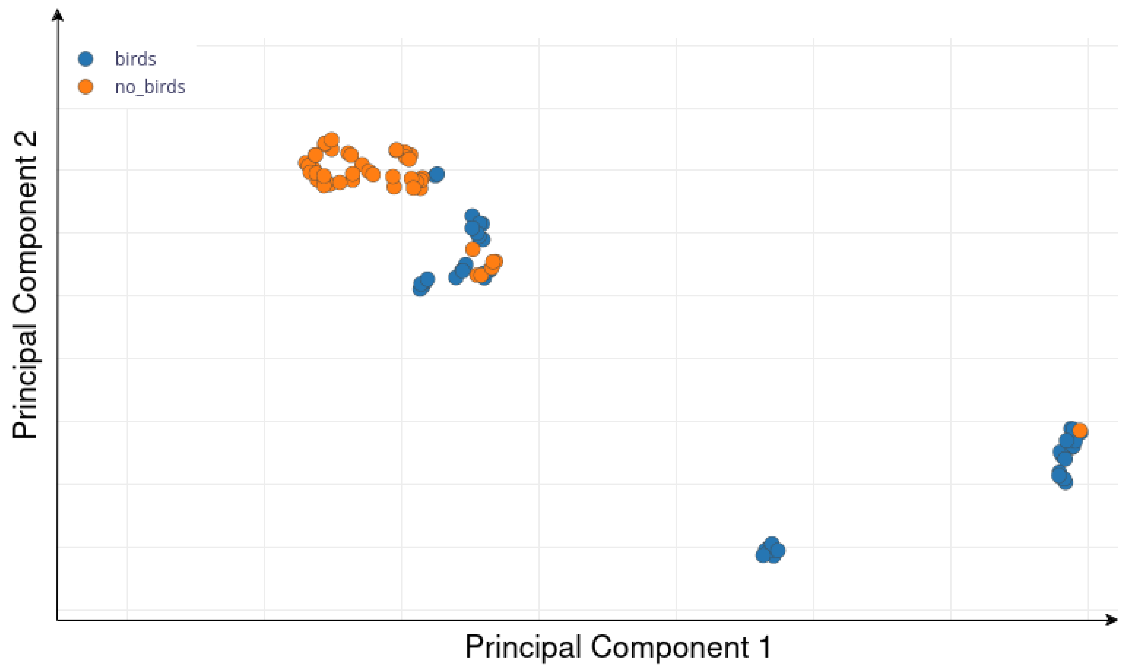
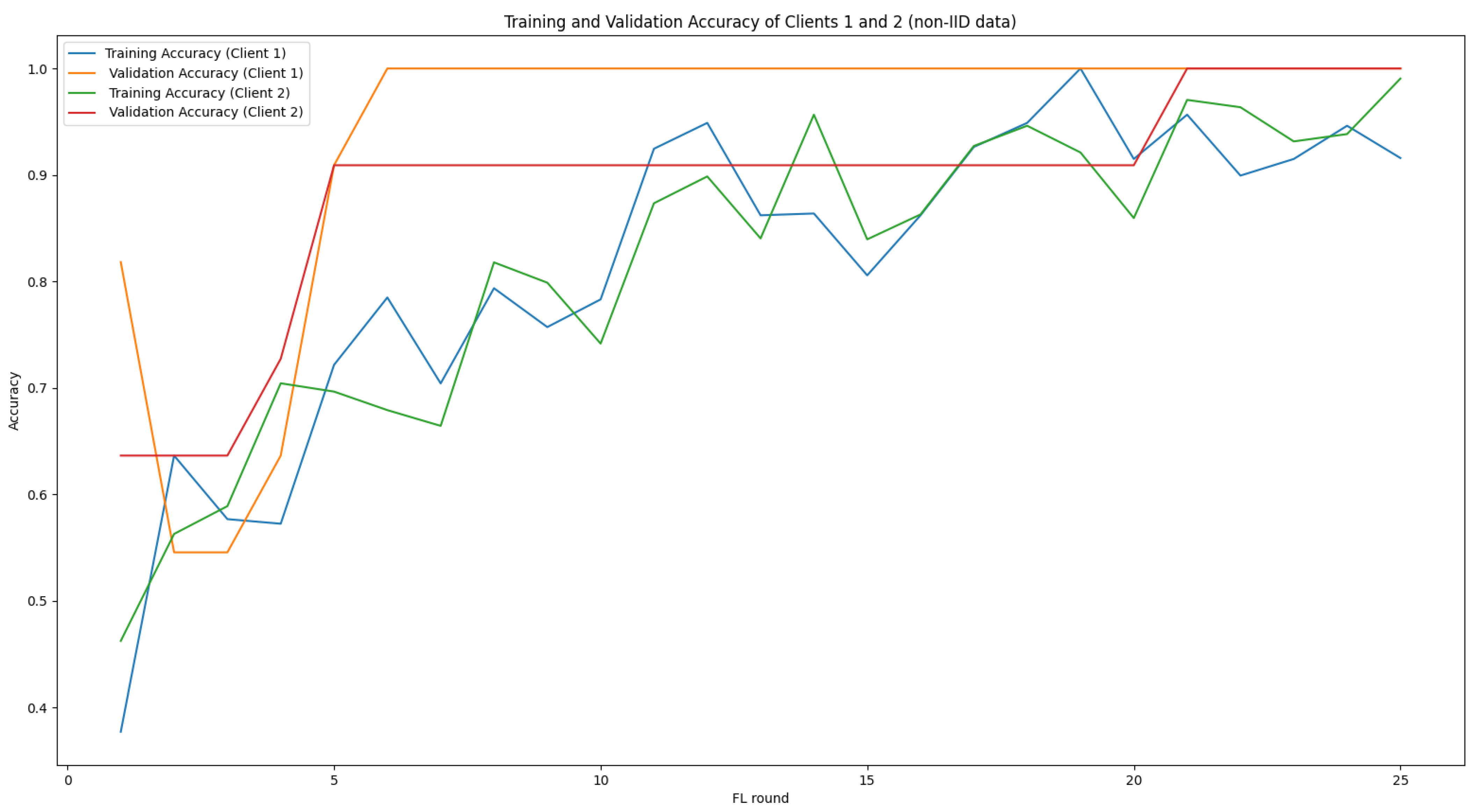
• Number of epochs: In one epoch, the model trains on the entire dataset. Too few epochs may lead to underfitting, while too many can result in overfitting. Given our small dataset, which has limited variability and is not very sparse in the feature space (Figure 6), a small number of epochs is sufficient to achieve model convergence. As shown in Figure 7, the model begins to overfit after the 11th epoch, with the validation accuracy plateauing while the training accuracy continues to rise. Based on this observation, we set the number of epochs to 11 to balance sufficient training while preventing overfitting. The model begins to overfit after a relatively small number of epochs, likely due to the limited size of the training dataset and the low diversity of samples, particularly those labeled as $no\_birds$.

To establish our benchmark performance, we first trained the model without fine-tuning and then fine-tuned the last 100 layers of MobileNetV2 for four more epochs.

Figure 8 presents the model confusion matrices in the test data set after training without fine-tuning and with fine-tuning, respectively. Fine-tuning offers limited advantages due to the simplicity of the classification task and the nature of the dataset used for training and testing. Utilizing the pre-trained MobileNetV2 for feature extraction is sufficient, as it effectively captures the necessary features. Training focuses solely on classifying the extracted features, enabling rapid learning. Fine-tuning additional layers in the base model does not result in significant improvements.

5.2. FL Preparation

To test our LEFL framework, we implemented an FL setup using hyperparameters derived from the benchmark configuration (Section 5.1) but adapted to fit the specific requirements of FL. These adaptations ensure compatibility with the federated environment while maintaining consistency with the benchmarking conditions.

• Batch size per client: In our FL scenario, each client is assigned 42 samples for training, which represents half of the base training dataset, as there are two clients. To accommodate this, we adjust the batch size by halving it. This results in a batch size of 8 samples per client.
• Base learning rate: Since we halved the batch size, we also reduced the learning rate by half to maintain learning behavior aligning with our benchmark. We set the base learning rate to $0.0005$ for each client.
• Optimizer: We kept the same optimizer as the benchmark (Adam) for both clients.
• Number of epochs per federated round: To maintain global control over the learning convergence, we ensured that each client performed one training pass per federated round. Therefore, we set the number of epochs to 1 for each client.
• Aggregation algorithm: Since we simulated a use case where both cameras monitor crop fields with equal importance and the training data are distributed equally across the clients, ensuring that no client has more weight than the other, we used the classic FedAvg algorithm with equal weights for all clients. The formula below illustrates the algorithm, with $w^{t+1}$ being the global weight at round $t+1$ and $w_1^t$ and $w_2^t$ being the local weights after round t of clients 1 and 2, respectively.

$$w^{t+1}={\displaystyle \frac{1}{2}}(w_1^t+w_2^t)$$

(3)

FedAvg stands out as the most suited algorithm for our study. FedSGD (federated stochastic gradient descent), for instance, transmits model gradients at every iteration, ensuring a more immediate synchronization of updates. However, this approach results in significant communication overhead, which is impractical in our low-energy, on-field training setup. FedProx, an extension of FedAvg that introduces a proximal term to stabilize updates in heterogeneous environments, could be beneficial in scenarios with highly diverse datasets, but given that our two cameras operate in similar agricultural conditions, such complexity is unnecessary. Scaffold, another alternative, attempts to correct model drift in non-IID settings by maintaining control variates but at the cost of additional computation and storage requirements, making it less suitable for our lightweight edge devices. FedOpt and other adaptive optimization-based methods, while promising for large-scale networks with diverse devices, introduce hyperparameter tuning challenges and increased computational costs that do not align with our goal of minimal energy expenditure. In contrast, FedAvg strikes the optimal balance for our scenario—it efficiently aggregates local model updates by averaging them at periodic intervals, significantly reducing communication overhead while maintaining convergence stability. Given that both cameras operate under similar conditions, the risk of model divergence is minimal, allowing FedAvg to perform effectively without additional complexity.

5.3. LEFL’s Performance

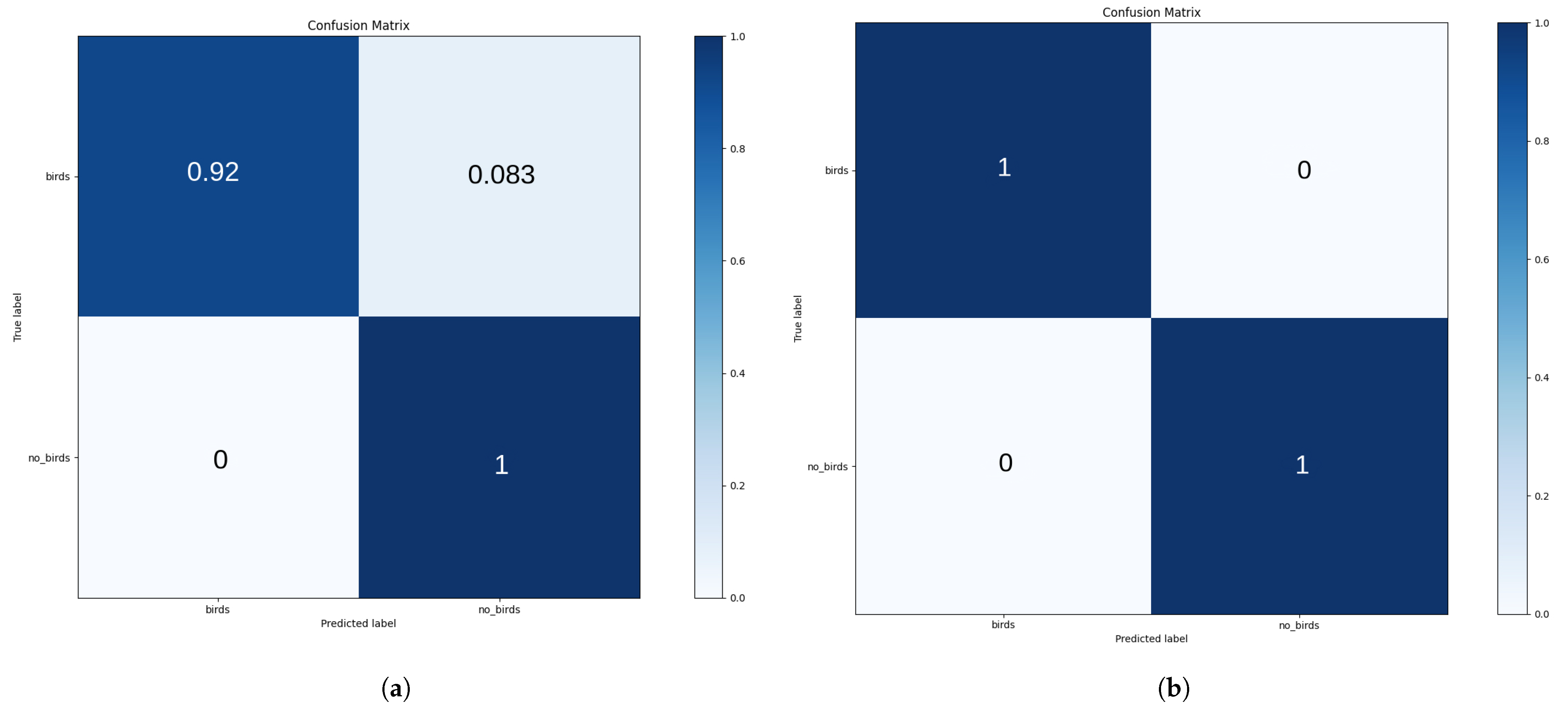
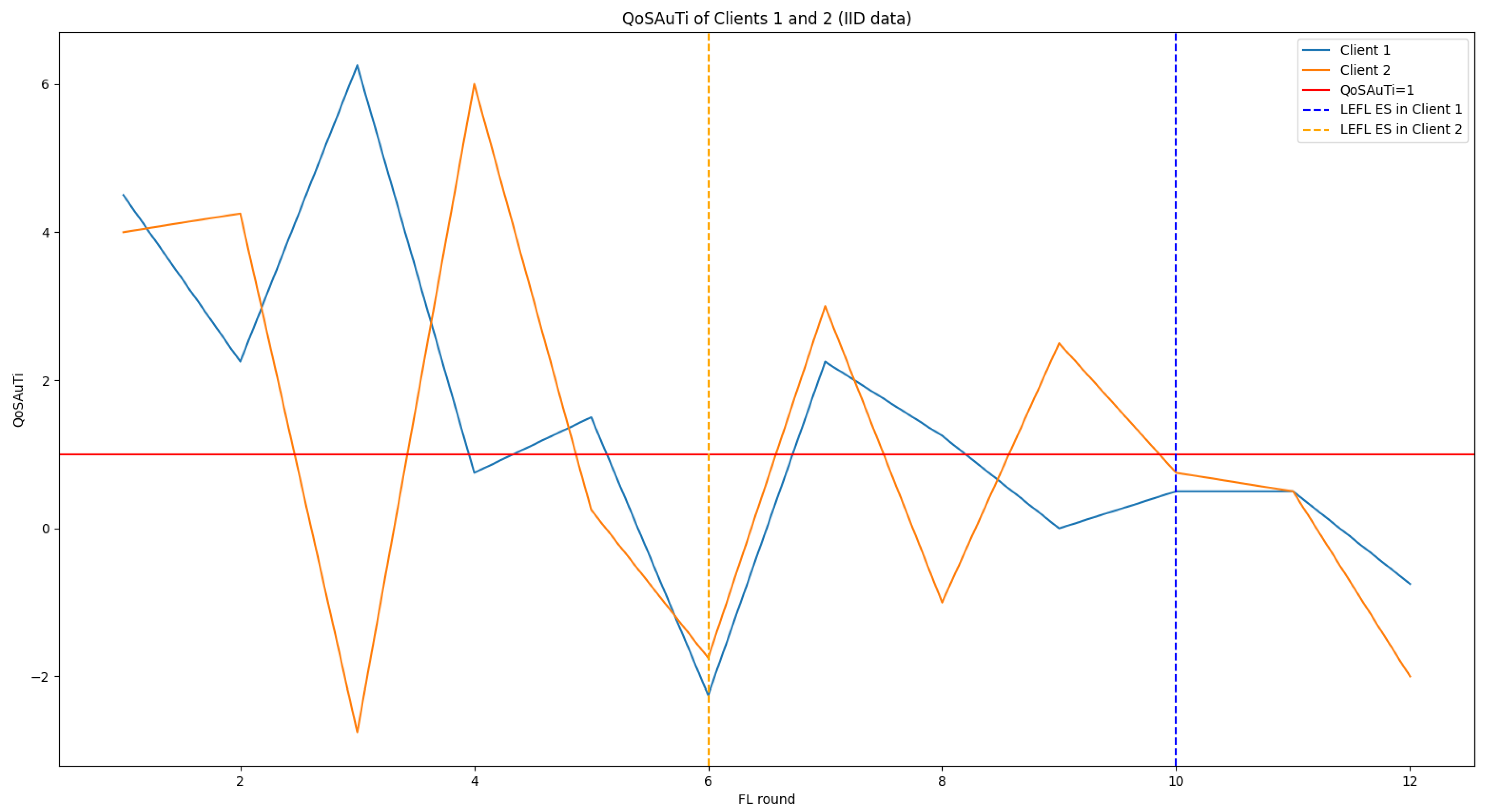
5.3.1. LEFL’s Performance on IID Data

To demonstrate the performance of our LEFL approach on an IID training dataset, we first trained our platform to achieve FL convergence, followed by training with LEFL.

Convergence is typically indicated when accuracies of local models converge, showing minimal improvement over subsequent training rounds. Figure 9 illustrates the training and validation accuracy for both clients 1 and 2 during 25 federated rounds within the IID data scenario. In this case, convergence was achieved in the 12th round, as shown in the figure. This result aligns with the benchmark’s convergence point (11th epoch) because the data are IID, ensuring that both clients (Client 1 and Client 2) share identical distributions and replicating the benchmark data distribution.

Figure 10 plots the $QoSAu{T}_i\left(k\right)$ (as defined in Section 3.1) in each round, i, for both clients ($k=\{1,2\}$) in the FL-to-convergence scenario, highlighting the specific round where the LEFL ES mechanism terminates the training. Each client exhibits a unique progression in its $QoSAu{T}_i$, driven by the inter-client diversity of the data. This diversity leads to distinct learning patterns as the model adapts locally within each client. The variation in learning patterns explains why the LEFL ES mechanism is triggered at different times for each client. It is important to note that the stopping criterion used in our LEFL ES mechanism, relying here on two consecutive $QoSAuT$ values (<1), can be adapted to the complexity of the considered models. This criterion should theoretically indicate that further training is no longer energy-efficient. In other use cases involving significantly larger datasets (e.g., 1000+ samples), our approach may prove suboptimal. In such cases, convergence may occur much later in higher rounds, and the $QoSAuT$ metric may experience temporary declines for several rounds (≥2) before subsequently improving and compensating for the earlier poor values. This is not the case in our use case, as convergence is reached quickly, causing the QoSAuT to decrease despite experiencing the fluctuations shortly after early stopping.

Figure 11 plots the confusion matrices of the global final model trained with LEFL and FL-to-convergence, respectively. In FL-to-convergence, we achieved results comparable to those of benchmark centralized learning without fine-tuning. However, in LEFL, accuracy is slightly reduced in favor of energy efficiency. This highlights the tradeoff enabled by LEFL between inference performance and energy-conscious training. It is worth noting that the accuracy of the model regarding the $no\_birds$ label did not decrease with LEFL. This is because partial convergence for this label was achieved earlier, given the limited diversity of its samples.

Table 11. Test accuracy and $QoSAuT$ of each device trained on IID data in three scenarios: LEFL, FL-to-convergence, and remote benchmark.

Scenario	LEFL	FL-to-Convergence	Remote Benchmark
Test Accuracy	0.91	0.96	0.96
$QoSAuT\left(1\right)$	1.55	1.40	0.09
$QoSAuT\left(2\right)$	2.56	1.40	0.09

summarizes the $QoSAuT$ (as defined in Section 3.1) for each device across three scenarios: LEFL, FL-to-convergence, and a classic remote benchmark training scheme. In the remote benchmark scheme, devices transmit their data to a remote server for centralized training under benchmark conditions (Section 5.1), with the resulting weights then deployed back to the devices for inference. All scenarios were evaluated under an IID data distribution.

FL improved the $QoSAuT$ of both clients by at least a factor of 15, primarily due to the significant reduction in the amount of data transmitted to the central server for training. Instead of transmitting large datasets as in the benchmark, FL keeps the data on edge devices, minimizing communication overhead. However, this advantage in reduced data transmission can be offset by increased computational costs if FL takes longer to converge, as is often the case in more complex scenarios. In our bird detection use case, FL appears particularly advantageous compared to traditional centralized training leaving limited room for further improvement via LEFL. As a result, LEFL slightly enhanced the $QoSAuT$. This enhancement varies between clients because the stopping mechanism was triggered at different rounds for each client.

It is important to note that the $QoSAuT$ of client 2 is influenced by client 1. After client 2 stopped training, it continued receiving updated weights from client 1, which was still learning, while maintaining its own training energy. This observation leads us to conclude that, in the context of FL, the $QoSAuT$ should be considered a global metric for the entire network, representing the average $QoSAuT$ of all clients. This approach accounts for the fact that each client’s performance is influenced by the participation of others in the training process, impacting their respective $QoSAuT$ values.

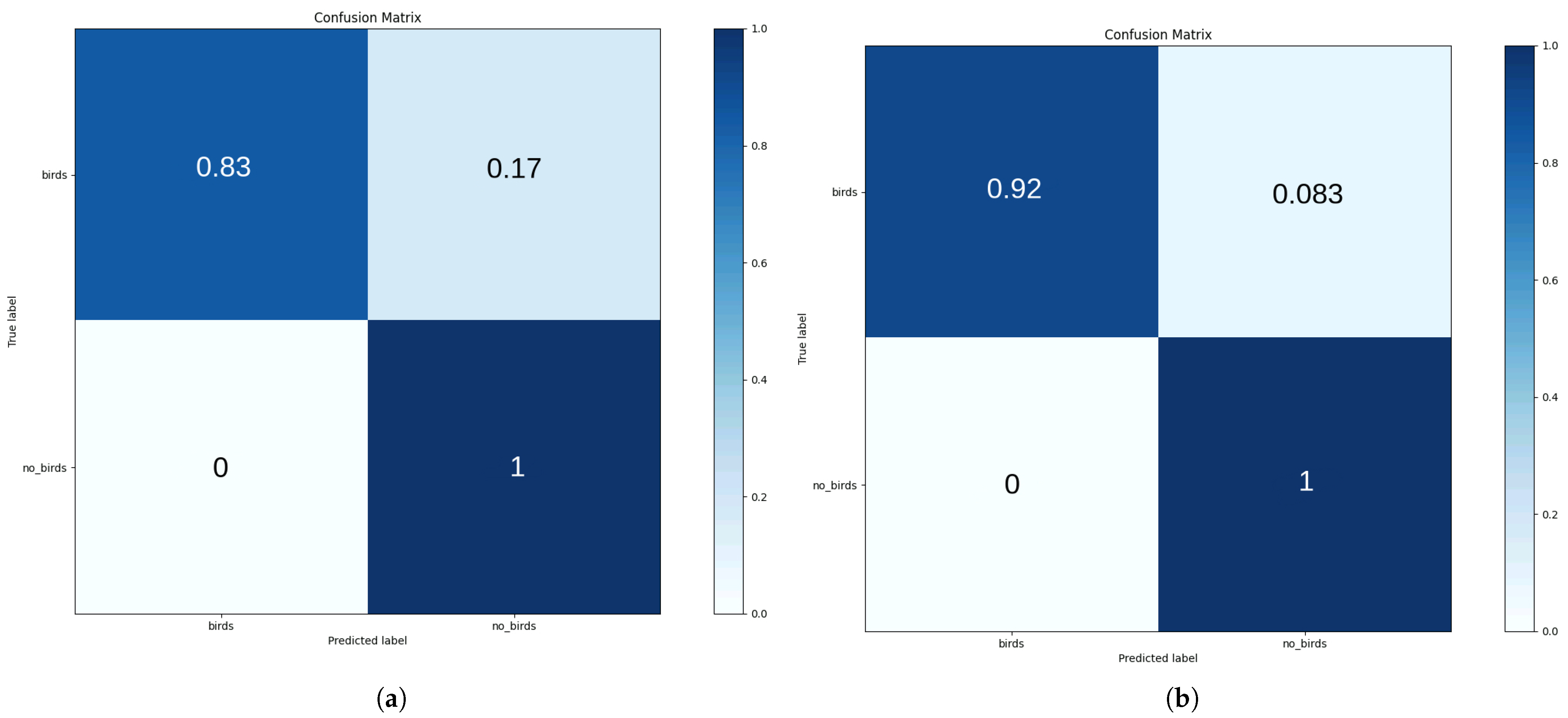
5.3.2. LEFL’s Performance on Non-IID Data

To demonstrate the performance of our LEFL approach on a non-IID training dataset, we first trained our platform to achieve FL convergence, followed by training with LEFL.

Figure 12 illustrates the training and validation accuracy for both clients 1 and 2 during 25 federated rounds within the non-IID data scenario. In this case, convergence occurred later compared to the IID data scenario, at the 22th round. This delayed convergence is attributed to the heterogeneous data distribution, which causes the client models to require more rounds to align and achieve consensus.

Figure 13 plots the $QoSAu{T}_i\left(k\right)$ in each round i for both clients ($k=\{1,2\}$) in the FL-to-convergence scenario, highlighting the specific round where LEFL ES mechanism terminates the training. $QoSAu{T}_i$ exhibits similar patterns to the IID data scenario, though it converges a few rounds later. However, the LEFL ES mechanism triggers as early as in the IID scenario, causing the model to learn less compared to the IID case.

Figure 14 plots the confusion matrices of the global final model trained with LEFL and FL-to-convergence, respectively. In the FL-to-convergence scenario, we achieved results comparable to those of FL-to-convergence and benchmark centralized learning with IID data. However, LEFL achieved lower accuracy compared to its performance in the IID data scenario due to the ES mechanism being triggered several rounds earlier than convergence, as convergence occurred later in the non-IID data scenario. It is important to note that the LEFL performance drop observed in the non-IID scenario compared to the IID scenario does not affect the $no\_bird$ label. This is because the samples for this label remain IID, even in the non-IID scenario, due to their lack of diversity in the dataset.

Table 12. Test accuracy and $QoSAuT$ of each device trained on non-IID data in three scenarios: LEFL, FL-to-convergence, and remote benchmark.

Scenario	LEFL	FL-to-Convergence	Remote Benchmark
Test Accuracy	0.87	0.96	0.96
$QoSAuT\left(1\right)$	1.44	0.77	0.09
$QoSAuT\left(2\right)$	1.80	0.77	0.09

summarizes the $QoSAuT$ for each device across 3 scenarios: LEFL, FL-to-convergence, and a classic remote benchmark training scheme. All scenarios are evaluated under a non-IID data distribution. However, it is important to highlight that, in the remote benchmark scenario, the data are inherently IID since they are centralized and aggregated on a server for training.

FL improved the $QoSAuT$ of both clients by at least a factor of 8. In the FL-to-convergence scenario, the improvement was smaller compared to the IID data scenario. This is because convergence occurred later with non-IID data, resulting in the $QoSAuT$ being reduced to half of that in the IID scenario to achieve the same model accuracy level. With LEFL, the model’s accuracy was lower due to the previously mentioned reasons (convergence occurred later in non-IID data). However, while the $QoSAuT$ was slightly lower than in the IID scenario, it remained at a comparable level (lower only by a factor of $1.1$ to $1.4$). Within the same non-IID data scenario, it is important to note, the $QoSAuT$ doubles in LEFL compared to FL-to-convergence. Comparing these two scenarios reveals that the model achieves only $9\%$ less accuracy but doubles the $QoSAuT$. This highlights the effectiveness of LEFL in optimizing the trade-off between accuracy and energy consumption. From a user’s perspective, agricultural devices that operate longer with slightly less accurate decisions can be more beneficial than devices that deliver higher accuracy but have a lifespan that is half as long.

The significant $QoSAuT$ improvements observed with FL-to-convergence compared to the benchmark—far exceeding the gains achieved using LEFL relative to FL-to-convergence—can be attributed to the simplicity of the classification task, the limited dataset diversity, and the small number of clients. These factors facilitate quicker convergence, even in non-IID data scenarios, compared to more complex tasks where data are more diverse and require more FL rounds to reach convergence. In more diverse non-IID data scenarios, LEFL is likely to exhibit even greater advantages in terms of $QoSAuT$ over the traditional FL-to-convergence training scheme.

6. Conclusions and Future Work

In this paper, we have proposed an Artificial Intelligence of Things (AIoT) system for bird detection in agricultural applications, with a strong focus on energy efficiency, particularly in terms of training costs. By leveraging federated learning (FL), we enhanced the energy efficiency of the system, reducing its energy consumption while maintaining the same decision-making quality. Furthermore, we also proposed a low-energy FL system (LEFL) in order to achieve a balance between decision quality and energy sobriety by stopping the FL training process earlier. To quantify decision-making quality, we used the model’s accuracy, and to evaluate energy efficiency, we introduced a novel metric, $QoSAuT$, which measures the quality of the service provided via our system in terms of decision-making. We tested our approach on a lightweight but realistic dataset obtained from real-world applications. This dataset consisted of around one hundred samples categorized into $birds$ and $no\_birds$ tailored for a simple classification task, which we distributed across our system in both IID and non-IID configurations to simulate potential scenarios that could occur during the training phase.

Training our designed system on the previously described dataset demonstrated a 15-fold improvement in energy efficiency using FL in the IID configuration and an eight-fold improvement in the non-IID configuration. With LEFL, the performance also improved slightly in IID scenarios with a low reduction in accuracy. However, a more significant improvement was achieved in non-IID scenarios with an also limited reduction in accuracy.

Our work presents a comprehensive approach to designing an energy-efficient, AIoT-based system for bird detection in agriculture 4.0. In future work, its robustness and scalability performances could be evaluated in more complex scenarios by diversifying the dataset, incorporating additional bird species, and broadening the feature diversity, such as including elements in the $no\_bird$ category like human presence or the presence of other animals and objects. However, composing the WSCN with two smart cameras is sufficient as a proof of concept, effectively demonstrating the LEFL advantages while remaining generalizable to networks with more nodes.

Additionally, the early stopping criteria used in our LEFL approach can be adapted to more complex tasks where FL convergence occurs significantly later than in our case. Future studies could explore alternative early stopping mechanisms, including methods for function approximation predicting the evolution of $QoSAuT$ to identify the point at which further rounds no longer contribute to enhancing the overall efficiency of the training process. Such forecasting could provide a more precise and effective stopping criterion.

Another strategy for improving the energy efficiency of our AIoT system is to optimize the inference phase by employing technologies with lower computational demands. This entails making thoughtful choices regarding both the hardware and the AI model in order to minimize resource consumption during inference. One possible path for hardware improvement is using neuromorphic vision sensors, also known as event-based or dynamic vision sensors (DVSs) [71]. These sensors capture only changes in the visual scene, enabling significant energy savings compared to the continuous frame-by-frame image capture of traditional cameras used in our system. From a model improvement perspective, spiking neural networks (SNNs) [72] are inherently event-driven, optimizing energy efficiency in local computations. This makes them particularly well-suited for processing event-based data from DVSs, enabling energy-efficient decision-making at the edge.

To further advance the bird detection use case and align it more closely with real-world agricultural/environmental requirements, semantic segmentation can be incorporated to not only improve the precision of bird detection but also quantify birds’ presence by accurately counting them in crop fields, thus estimating the scale of potential losses caused. An energy-efficient approach to addressing this involves both optimized hardware and an adapted model, as discussed earlier, by training a wireless DVS network powered via an SNN model for semantic segmentation. Additionally, integrating LEFL could further improve training efficiency, making the system energy-efficient in both the training and inference phases.

EvSegSNN [73] successfully combines SNNs with DVSs to perform semantic segmentation, demonstrating promising results from an energy-efficient standpoint. Implementing this approach in the bird detection scenario, while incorporating LEFL for energy-efficient training, could be an exciting research direction.

References

- Basso, B.; Antle, J. Digital agriculture to design sustainable agricultural systems. Nat. Sustain. 2020, 3, 254–256. [Google Scholar] [CrossRef]
- Wakchaure, M.; Patle, B.; Mahindrakar, A. Application of AI techniques and robotics in agriculture: A review. Artif. Intell. Life Sci. 2023, 3, 100057. [Google Scholar] [CrossRef]
- Eli-Chukwu, N.C. Applications of Artificial Intelligence in Agriculture: A Review. Eng. Technol. Appl. Sci. Res. 2019, 9, 4377–4383. [Google Scholar] [CrossRef]
- Lytridis, C.; Kaburlasos, V.G.; Pachidis, T.; Manios, M.; Vrochidou, E.; Kalampokas, T.; Chatzistamatis, S. An Overview of Cooperative Robotics in Agriculture. Agronomy 2021, 11, 1818. [Google Scholar] [CrossRef]
- Farooq, M.S.; Riaz, S.; Abid, A.; Umer, T.; Zikria, Y.B. Role of IoT Technology in Agriculture: A Systematic Literature Review. Electronics 2020, 9, 319. [Google Scholar] [CrossRef]
- Banđur, D.; Jakšić, B.; Banđur, M.; Jović, S. An analysis of energy efficiency in Wireless Sensor Networks (WSNs) applied in smart agriculture. Comput. Electron. Agric. 2019, 156, 500–507. [Google Scholar] [CrossRef]
- Raghunathan, V.; Schurgers, C.; Park, S.; Srivastava, M. Energy-aware wireless microsensor networks. IEEE Signal Process. Mag. 2002, 19, 40–50. [Google Scholar] [CrossRef]
- Jawad, H.; Nordin, R.; Gharghan, S.; Jawad, A.; Ismail, M. Energy-Efficient Wireless Sensor Networks for Precision Agriculture: A Review. Sensors 2017, 17, 1781. [Google Scholar] [CrossRef]
- Sahota, H.; Kumar, R.; Kamal, A.; Huang, J. An energy-efficient wireless sensor network for precision agriculture. In Proceedings of the IEEE Symposium on Computers and Communications, Riccione, Italy, 22–25 June 2010; IEEE: Piscataway, NJ, USA, 2010; pp. 347–350. [Google Scholar] [CrossRef]
- Hemmati, A.; Rahmani, A.M. The Internet of Autonomous Things applications: A taxonomy, technologies, and future directions. Internet Things 2022, 20, 100635. [Google Scholar] [CrossRef]
- Singh, R.; Gill, S.S. Edge AI: A survey. Internet Things Cyber-Phys. Syst. 2023, 3, 71–92. [Google Scholar] [CrossRef]
- Kukreja, N.; Shilova, A.; Beaumont, O.; Huckelheim, J.; Ferrier, N.; Hovland, P.; Gorman, G. Training on the Edge: The why and the how. arXiv 2019, arXiv:1903.03051. [Google Scholar]
- Shi, Y.; Yang, K.; Jiang, T.; Zhang, J.; Letaief, K.B. Communication-Efficient Edge AI: Algorithms and Systems. arXiv 2020, arXiv:2002.09668. [Google Scholar]
- McMahan, H.B.; Moore, E.; Ramage, D.; Hampson, S.; Arcas, B.A.y. Communication-Efficient Learning of Deep Networks from Decentralized Data. arXiv 2016, arXiv:1602.05629. [Google Scholar]
- Zhang, C.; Xie, Y.; Bai, H.; Yu, B.; Li, W.; Gao, Y. A survey on federated learning. Knowl.-Based Syst. 2021, 216, 106775. [Google Scholar] [CrossRef]
- Zhu, H.; Xu, J.; Liu, S.; Jin, Y. Federated Learning on Non-IID Data: A Survey. arXiv arXiv:cs.LG/2106.06843, 2021.
- Zhao, Y.; Li, M.; Lai, L.; Suda, N.; Civin, D.; Chandra, V. Federated Learning with Non-IID Data. arXiv 2018, arXiv:1806.00582. [Google Scholar]
- Zhao, Z.; Feng, C.; Hong, W.; Jiang, J.; Jia, C.; Quek, T.Q.S.; Peng, M. Federated Learning with Non-IID Data in Wireless Networks. IEEE Trans. Wirel. Commun. 2022, 21, 1927–1942. [Google Scholar] [CrossRef]
- Restrepo-Arias, J.F.; Branch-Bedoya, J.W.; Awad, G. Image classification on smart agriculture platforms: Systematic literature review. Artif. Intell. Agric. 2024, 13, 1–17. [Google Scholar] [CrossRef]
- Liu, G.; Zhong, K.; Li, H.; Chen, T.; Wang, Y. A state of art review on time series forecasting with machine learning for environmental parameters in agricultural greenhouses. Inf. Process. Agric. 2024, 11, 143–162. [Google Scholar] [CrossRef]
- Jha, K.; Doshi, A.; Patel, P.; Shah, M. A comprehensive review on automation in agriculture using artificial intelligence. Artif. Intell. Agric. 2019, 2, 1–12. [Google Scholar] [CrossRef]
- Xu, J.; Gu, B.; Tian, G. Review of agricultural IoT technology. Artif. Intell. Agric. 2022, 6, 10–22. [Google Scholar] [CrossRef]
- Qazi, S.; Khawaja, B.A.; Farooq, Q.U. IoT-Equipped and AI-Enabled Next Generation Smart Agriculture: A Critical Review, Current Challenges and Future Trends. IEEE Access 2022, 10, 21219–21235. [Google Scholar] [CrossRef]
- Muhammed, D.; Ahvar, E.; Ahvar, S.; Trocan, M.; Montpetit, M.J.; Ehsani, R. Artificial Intelligence of Things (AIoT) for smart agriculture: A review of architectures, technologies and solutions. J. Netw. Comput. Appl. 2024, 228, 103905. [Google Scholar] [CrossRef]
- Kumar, S.; Chowdhary, G.; Udutalapally, V.; Das, D.; Mohanty, S.P. gCrop: Internet-of-Leaf-Things (IoLT) for Monitoring of the Growth of Crops in Smart Agriculture. In Proceedings of the 2019 IEEE International Symposium on Smart Electronic Systems (iSES) (Formerly iNiS), Rourkela, India, 16–18 December 2019; pp. 53–56. [Google Scholar] [CrossRef]
- T, M.; Makkithaya, K.; G, N.V. A Federated Learning-Based Crop Yield Prediction for Agricultural Production Risk Management. In Proceedings of the 2022 IEEE Delhi Section Conference (DELCON), New Delhi, India, 11–13 February 2022; IEEE: Piscataway, NJ, USA, 2022. [Google Scholar] [CrossRef]
- Yu, C.; Shen, S.; Zhang, K.; Zhao, H.; Shi, Y. Energy-Aware Device Scheduling for Joint Federated Learning in Edge-assisted Internet of Agriculture Things. In Proceedings of the 2022 IEEE Wireless Communications and Networking Conference (WCNC), Austin, TX, USA, 10–13 April 2022; IEEE: Piscataway, NJ, USA, 2022. [Google Scholar] [CrossRef]
- Idoje, G.; Dagiuklas, T.; Iqbal, M. Federated Learning: Crop classification in a smart farm decentralised network. Smart Agric. Technol. 2023, 5, 100277. [Google Scholar] [CrossRef]
- Jiang, P.; Chen, Y.; Liu, B.; He, D.; Liang, C. Real-Time Detection of Apple Leaf Diseases Using Deep Learning Approach Based on Improved Convolutional Neural Networks. IEEE Access 2019, 7, 59069–59080. [Google Scholar] [CrossRef]
- Antico, T.M.; Moreira, L.F.R.; Moreira, R. Evaluating the Potential of Federated Learning for Maize Leaf Disease Prediction. In Proceedings of the Anais do XIX Encontro Nacional de Inteligência Artificial e Computacional (ENIAC 2022), Sociedade Brasileira de Computação—SBC, 2022, ENIAC 2022, Campinas, Brazil, 28 November–1 December; 2022. [Google Scholar] [CrossRef]
- Khan, F.S.; Khan, S.; Mohd, M.N.H.; Waseem, A.; Khan, M.N.A.; Ali, S.; Ahmed, R. Federated learning-based UAVs for the diagnosis of Plant Diseases. In Proceedings of the 2022 International Conference on Engineering and Emerging Technologies (ICEET), Kuala Lumpur, Malaysia, 27–28 October 2022; IEEE: Piscataway, NJ, USA, 2022. [Google Scholar] [CrossRef]
- Patros, P.; Ooi, M.; Huang, V.; Mayo, M.; Anderson, C.; Burroughs, S.; Baughman, M.; Almurshed, O.; Rana, O.; Chard, R.; et al. Rural AI: Serverless-Powered Federated Learning for Remote Applications. IEEE Internet Comput. 2023, 27, 28–34. [Google Scholar] [CrossRef]
- Deng, F.; Mao, W.; Zeng, Z.; Zeng, H.; Wei, B. Multiple Diseases and Pests Detection Based on Federated Learning and Improved Faster R-CNN. IEEE Trans. Instrum. Meas. 2022, 71, 3523811. [Google Scholar] [CrossRef]
- Vincent, D.R.; Deepa, N.; Elavarasan, D.; Srinivasan, K.; Chauhdary, S.H.; Iwendi, C. Sensors Driven AI-Based Agriculture Recommendation Model for Assessing Land Suitability. Sensors 2019, 19, 3667. [Google Scholar] [CrossRef]
- Murugamani, C.; Shitharth, S.; Hemalatha, S.; Kshirsagar, P.R.; Riyazuddin, K.; Naveed, Q.N.; Islam, S.; Mazher Ali, S.P.; Batu, A. Machine Learning Technique for Precision Agriculture Applications in 5G-Based Internet of Things. Wirel. Commun. Mob. Comput. 2022, 2022, 6534238. [Google Scholar] [CrossRef]
- Dahane, A.; Benameur, R.; Kechar, B.; Benyamina, A. An IoT Based Smart Farming System Using Machine Learning. In Proceedings of the 2020 International Symposium on Networks, Computers and Communications (ISNCC), Montreal, QC, Canada, 20–22 October 2020; pp. 1–6. [Google Scholar] [CrossRef]
- Cheng, Z.; Zhang, F. Flower End-to-End Detection Based on YOLOv4 Using a Mobile Device. Wirel. Commun. Mob. Comput. 2020, 2020, 1–9. [Google Scholar] [CrossRef]
- Hsu, C.W.; Huang, Y.H.; Huang, N.F. Real-time Dragonfruit’s Ripeness Classification System with Edge Computing Based on Convolution Neural Network. In Proceedings of the 2022 International Conference on Information Networking (ICOIN), Jeju-si, Republic of Korea, 12–15 January 2022; IEEE: Piscataway, NJ, USA, 2022; pp. 177–182. [Google Scholar] [CrossRef]
- Paul, P.B.; Biswas, S.; Bairagi, A.K.; Masud, M. Data-Driven Decision Making for Smart Cultivation. In Proceedings of the 2021 IEEE International Symposium on Smart Electronic Systems (iSES), Jaipur, India, 18–22 December 2021; IEEE: Piscataway, NJ, USA, 2021; pp. 249–254. [Google Scholar] [CrossRef]
- Arablouei, R.; Wang, L.; Currie, L.; Yates, J.; Alvarenga, F.A.; Bishop-Hurley, G.J. Animal behavior classification via deep learning on embedded systems. Comput. Electron. Agric. 2023, 207, 107707. [Google Scholar] [CrossRef]
- Mao, A.; Huang, E.; Gan, H.; Liu, K. FedAAR: A Novel Federated Learning Framework for Animal Activity Recognition with Wearable Sensors. Animals 2022, 12, 2142. [Google Scholar] [CrossRef] [PubMed]
- Aliahmadi, A.; Nozari, H.; Ghahremani-Nahr, J. AIoT-based Sustainable Smart Supply Chain Framework. Int. J. Innov. Manag. Econ. Soc. Sci. 2022, 2, 28–38. [Google Scholar] [CrossRef]
- Durrant, A.; Markovic, M.; Matthews, D.; May, D.; Enright, J.; Leontidis, G. The role of cross-silo federated learning in facilitating data sharing in the agri-food sector. Comput. Electron. Agric. 2022, 193, 106648. [Google Scholar] [CrossRef]
- Chabot, D.; Francis, C.M. Computer-automated bird detection and counts in high-resolution aerial images: A review. J. Field Ornithol. 2016, 87, 343–359. [Google Scholar] [CrossRef]
- Akçay, H.G.; Kabasakal, B.; Aksu, D.; Demir, N.; Öz, M.; Erdoğan, A. Automated Bird Counting with Deep Learning for Regional Bird Distribution Mapping. Animals 2020, 10, 1207. [Google Scholar] [CrossRef]
- Wäldchen, J.; Mäder, P. Machine learning for image based species identification. Methods Ecol. Evol. 2018, 9, 2216–2225. [Google Scholar] [CrossRef]
- Hong, S.J.; Han, Y.; Kim, S.Y.; Lee, A.Y.; Kim, G. Application of Deep-Learning Methods to Bird Detection Using Unmanned Aerial Vehicle Imagery. Sensors 2019, 19, 1651. [Google Scholar] [CrossRef]
- Lee, S.; Lee, M.; Jeon, H.; Smith, A. Bird Detection in Agriculture Environment using Image Processing and Neural Network. In Proceedings of the 2019 6th International Conference on Control, Decision and Information Technologies (CoDIT), Paris, France, 23–26 April 2019; pp. 1658–1663. [Google Scholar] [CrossRef]
- Li, C.; Zhang, B.; Hu, H.; Dai, J. Enhanced Bird Detection from Low-Resolution Aerial Image Using Deep Neural Networks. Neural Process. Lett. 2018, 49, 1021–1039. [Google Scholar] [CrossRef]
- Mashuk, F.; Sattar, A.; Sultana, N. Machine Learning Approach for Bird Detection. In Proceedings of the 2021 Third International Conference on Intelligent Communication Technologies and Virtual Mobile Networks (ICICV), Tirunelveli, India, 4–6 February 2021; IEEE: Piscataway, NJ, USA, 2021; pp. 818–822. [Google Scholar] [CrossRef]
- Nguyen, D.C.; Pham, Q.V.; Pathirana, P.N.; Ding, M.; Seneviratne, A.; Lin, Z.; Dobre, O.; Hwang, W.J. Federated Learning for Smart Healthcare: A Survey. ACM Comput. Surv. 2022, 55, 1–37. [Google Scholar] [CrossRef]
- Zhou, J.; Zhang, S.; Lu, Q.; Dai, W.; Chen, M.; Liu, X.; Pirttikangas, S.; Shi, Y.; Zhang, W.; Herrera-Viedma, E. A Survey on Federated Learning and its Applications for Accelerating Industrial Internet of Things. arXiv 2021, arXiv:2104.10501. [Google Scholar]
- Pandya, S.; Srivastava, G.; Jhaveri, R.; Babu, M.R.; Bhattacharya, S.; Maddikunta, P.K.R.; Mastorakis, S.; Piran, M.J.; Gadekallu, T.R. Federated learning for smart cities: A comprehensive survey. Sustain. Energy Technol. Assess. 2023, 55, 102987. [Google Scholar] [CrossRef]
- Žalik, K.R.; Žalik, M. A Review of Federated Learning in Agriculture. Sensors 2023, 23, 9566. [Google Scholar] [CrossRef] [PubMed]
- Saha, R.; Misra, S.; Deb, P.K. FogFL: Fog-Assisted Federated Learning for Resource-Constrained IoT Devices. IEEE Internet Things J. 2021, 8, 8456–8463. [Google Scholar] [CrossRef]
- Kumar, A.; Srirama, S.N. Fog Enabled Distributed Training Architecture for Federated Learning. In Big Data Analytics; Springer International Publishing: Berlin/Heidelberg, Germany, 2021; pp. 78–92. [Google Scholar] [CrossRef]
- Kumar, P.; Gupta, G.P.; Tripathi, R. PEFL: Deep Privacy-Encoding-Based Federated Learning Framework for Smart Agriculture. IEEE Micro 2022, 42, 33–40. [Google Scholar] [CrossRef]
- Friha, O.; Ferrag, M.A.; Shu, L.; Maglaras, L.; Choo, K.K.R.; Nafaa, M. FELIDS: Federated learning-based intrusion detection system for agricultural Internet of Things. J. Parallel Distrib. Comput. 2022, 165, 17–31. [Google Scholar] [CrossRef]
- Abu-Khadrah, A.; Ali, A.M.; Jarrah, M. An Amendable Multi-Function Control Method using Federated Learning for Smart Sensors in Agricultural Production Improvements. ACM Trans. Sens. Netw. 2023. [Google Scholar] [CrossRef]
- Sachidananda, V.; Khelil, A.; Suri, N. Quality of information in wireless sensor networks: A survey. Citeseer 2010. [Google Scholar]
- Dong, K.; Zhou, C.; Ruan, Y.; Li, Y. MobileNetV2 Model for Image Classification. In Proceedings of the 2020 2nd International Conference on Information Technology and Computer Application (ITCA), Guangzhou, China, 18–20 December 2020; IEEE: Piscataway, NJ, USA, 2020; pp. 476–480. [Google Scholar] [CrossRef]
- Gupta, J.; Pathak, S.; Kumar, G. Deep Learning (CNN) and Transfer Learning: A Review. J. Phys. Conf. Ser. 2022, 2273, 012029. [Google Scholar] [CrossRef]
- Abadi, M.; Barham, P.; Chen, J.; Chen, Z.; Davis, A.; Dean, J.; Devin, M.; Ghemawat, S.; Irving, G.; Isard, M.; et al. TensorFlow: A system for large-scale machine learning. arXiv 2016, arXiv:1605.08695. [Google Scholar]
- Beutel, D.J.; Topal, T.; Mathur, A.; Qiu, X.; Fernandez-Marques, J.; Gao, Y.; Sani, L.; Li, K.H.; Parcollet, T.; de Gusmão, P.P.B.; et al. Flower: A Friendly Federated Learning Research Framework. arXiv 2020, arXiv:2007.14390. [Google Scholar]
- Stuecke, J. Top 7 Open-Source Frameworks for Federated Learning. 2024. Available online: https://www.apheris.com/resources/blog/top-7-open-source-frameworks-for-federated-learning/ (accessed on 13 December 2024).
- Niu, Z.; Dong, H.; Qin, A.K.; Gu, T. FLrce: Resource-Efficient Federated Learning with Early-Stopping Strategy. arXiv 2023, arXiv:2310.09789. [Google Scholar]
- Sausse, C.; Barbu, C.; Bertrand, M.; Thibord, J.B. Dégâts d’oiseaux à la levée: Vers un changement de méthode? Phytoma 2022, 35–38. [Google Scholar]
- Ferreboeuf, H. The Shift Project, Lean ICT Report. 2018. Available online: https://theshiftproject.org/en/article/lean-ict-our-new-report/ (accessed on 12 December 2024).
- Sevilla, J.; Heim, L.; Hobbhahn, M.; Besiroglu, T.; Ho, A.; Villalobos, P. Estimating Training Compute of Deep Learning Models. 2022. Available online: https://epoch.ai/blog/estimating-training-compute (accessed on 18 December 2024).
- Sandler, M.; Howard, A.; Zhu, M.; Zhmoginov, A.; Chen, L.C. MobileNetV2: Inverted Residuals and Linear Bottlenecks. arXiv 2018, arXiv:1801.04381. [Google Scholar]
- Liao, F.; Zhou, F.; Chai, Y. Neuromorphic vision sensors: Principle, progress and perspectives. J. Semicond. 2021, 42, 013105. [Google Scholar] [CrossRef]
- Ghosh-Dastidar, S.; Adeli, H. Spiking neural networks. Int. J. Neural Syst. 2009, 19, 295–308. [Google Scholar] [CrossRef]
- Hareb, D.; Martinet, J. EvSegSNN: Neuromorphic Semantic Segmentation for Event Data. arXiv 2024, arXiv:2406.14178. [Google Scholar]