Stability of Heterogeneous Beams with Three Supports—Solutions Using Integral Equations

Abstract

It is our main objective to find the critical load for three beams with cross sectional heterogeneity. Each beam has three supports, of which the intermediate one is a spring support. Determination of the critical load for these beams leads to three point boundary value problems (BVPs) associated with homogeneous boundary conditions—the mentioned BVPs constitute three eigenvalue problems. They are solved by using a novel solution strategy based on the Green functions that belong to these BVPs: the eigenvalue problems established for the critical load are transformed into eigenvalue problems governed by homogeneous Fredholm integral equations with kernels that can be given in closed forms provided that the Green function of each BVP is known. Then the eigenvalue problems governed by the Fredholm integral equations can be manipulated into algebraic eigenvalue problems solved numerically by using effective algorithms. It is an advantage of the way we attack these problems that the formalism established and the results obtained remain valid for homogeneous beams as well. The numerical results for the critical forces can be applied to solve some stability problems in the engineering practice.

1. Introduction

Buckling of structures and various structural members has been subject to research for a long time and is still a popular topic [1,2,3,4]. When it comes to the stability of beams or columns, the number of available works is numerous. Notable articles [5,6,7,8] are subject to the elastic stability of axially loaded beams. Not only analytical but also numerical and experimental findings are available. In [9], the effect of end-restraints—by means of linear rotational and translational springs—on the critical load is investigated. A novel variational-iterational method is provided in [10] that is applicable even for non-uniform cross-sections. Meanwhile, model [11] further incorporates functionally graded material distribution. Such beams can identically be replaced with beams whose material and geometrical properties are constant. In [12] the buckling of an inextensible column is in the spotlight. A novel solution of the governing non-linear equation, namely the Adomian decomposition method is presented through the Green function technique. The clear advantage of this method is that, while being rapid, non-linear problems can be solved without needing to use the perturbation theory. Material nonlinearity is included in [13] when the spatial buckling of nanorods and nanotubes is investigated. The material law is the helical Cauchy-Born rule. Interesting results are related to the stability problem of the von Mises truss in [14] by taking into account the geometric and material nonlinearity and the shear deformation as well.

Article [15] is about the buckling of straight Euler-Bernoulli beams with two supports. Two approaches are detailed in this work, one of these is based on an integral equation whose kernel is the Green function. The Green function is computed numerically. Other notable findings are mentioned about geometrically imperfect columns, which are addressed theoretically and experimentally in articles [16,17] to find the sensitivity of the buckling loads under these circumstances. Apart from buckling, it is worthy to mention some further results about the Green function. Early book [18] defines the Green function itself and presents applications to electricity and magnetism. Since that pioneering work, the Green function has widely been applied to various problems [19,20].

The Green function was introduced in [21] with possible applications to two-point BVPs determined by ODEs. Furthermore, there are books [22,23,24] that deal with the generalization of the Green function for a given class of differential equations (DE). In relation with degenerated ordinary differential equation systems, some new findings are reported in [25]. The existence of some three-point BVPs determined by non-linear DEs of order three is assessed in [26] by means of Green functions. In [27], for a class of ordinary differential equations of order two, a method is presented in order to find the Green functions for three-point BVPs. Paper [28] is dedicated to a specific class of third-order three-point BVPs. A technique is detailed about how to find the Green function. A kind of non-linear third-order non-local BVP problem is investigated in [29], where the Schauder fixed point theorem is used in order to get a solution. A non-local three-point BVP is examined in [30]. Existence and uniqueness of solutions are proven and the corresponding Green function is also constructed. A third-order linear differential equation is investigated in [31]. The existence of the Green function is proven and solution is given.

This work is dedicated to the linear stability problem of three partially elastically supported beams. The results obtained are the generalizations of similar investigations presented in paper [32] for ideal, rigid supports. Accordingly, the beams in question have cross-sectional inhomogeneity and are supported at three different points—the corresponding mathematical problems are three-point BVPs. The applied procedure requires the solution of Fredholm integral equations with kernels constituted by the second derivative of the related Green functions. Thus, the Green functions should also be determined.A boundary element approach is used in order to find numerical solution to the issue in question. In general, the position of the middle support has significant effects on the ultimate load bearing abilities.

As regards the problems attacked in this article, it should be noted that the relevant formulation is a classical one. However, the difference in contrast to the classical formulation of these problems is that the material of the beams is not homogeneous and the solution procedure is also novel, as it is based on the use of integral equations.

The paper is organized in eight sections. After the Introduction, Section 2 gathers the most important assumptions and the typical equilibrium equations. Section 3 clarifies the properties of the Green functions for the considered three point eigenvalue problems and provide their calculations. Section 4 presents the kernels of the integral equations that can be utilized for finding the critical axial forces. Computational results are given in Section 5 both in tabular and graphical format to reveal the effects of the end supports and spring stiffness. Finally, the Section 6 and Appendix A conclude the manuscript.

2. Differential Equations

Governing Equations

We shall consider three heterogeneous beams of length L with uniform cross-section shown in Figure 1. The axial force N ($N>0$) is compressive. The first beam is a fixed-fixed beam with an intermediate spring support (FssF beam), the second is a fixed-pinned beam also with an intermediate support (FssP beam) and the third is a pinned-pinned beam which also has an intermediate spring support (PssP beam). If the intermediate support is a roller the beams are referred to as FrF, FrP and PrP beams. The E-weighted centerline (called centerline for brevity) of each beam coincides with axis $\widehat{x}$ of the coordinate system $\widehat{x},\widehat{y},\widehat{z}$. Note that the E-weighted first moment $Q_{\widehat{y}}$ is zero in this coordinate system [32,33]:

$$Q_{\widehat{y}}={\int }_A\widehat{z}E(\widehat{y},\widehat{z})\mathrm{d}A=0.$$

(1)

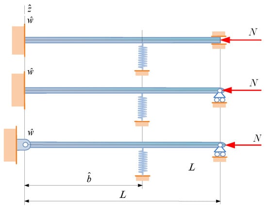
Figure 1. Fixed-fixed, fixed-pinned and pinned-pinned beams each with an intermediate spring support.

We shall assume that the coordinate plane $\widehat{x}\widehat{z}$ is a symmetry plane of the beams not only in geometry but also in material distribution. The modulus of elasticity E can vary as $E(\widehat{y},\widehat{z})=E(-\widehat{y},\widehat{z})$—it is, therefore, independent of $\widehat{x}$. Besides the end-supports, the intermediate one is placed at the coordinate denoted by $\widehat{b}$.

As is well known the simple equilibrium problems of these non-homogeneous beams are governed by the ordinary differential equation (ODE) [33]:

$$\frac{{\mathrm{d}}^4\widehat{w}}{\mathrm{d}\widehat{x}{}^4}=\frac{{\widehat{f}}_z}{I_{ey}}$$

(2)

with $\widehat{w}$ being the transversal displacement, while ${\widehat{f}}_z\left(x\right)$ is the distributed load and $I_{ey}$ is defined by the equation

$$I_{ey}={\int }_{A}E(\widehat{y},\widehat{z})z^2\mathrm{d}A.$$

(3)

Let $\widehat{\xi }$ be also a coordinate measured on the centerline with the same origin the coordinate $\widehat{x}$ has—$\widehat{\xi }$ is independent of $\widehat{x}$. In what follows we shall use the dimensionless variables:

$$\begin{array}{c}x=\widehat{x}/L,\xi =\widehat{\xi }/L,w=\widehat{w}/L,\\ y=\frac{\mathrm{d}\widehat{w}}{\mathrm{d}\widehat{x}}=\frac{\mathrm{d}w}{\mathrm{d}x},b=\widehat{b}/\widehat{L},\ell ={\left.\frac{x}{L}\right|}_{x=L}=1,\end{array}$$

(4)

Therefore, Equation (2) becomes

$$\frac{{\mathrm{d}}^{4}w}{\mathrm{d}{x}^4}=f_z,f_z=\frac{L^3{\widehat{f}}_z}{I_{ey}}$$

(5)

which is paired with the typical boundary and continuity conditions given in Table 1.

Table 1. Boundary and continuity conditions.

Boundary Conditions
(FssF beam)	(FssP beam)	(PssP beam)
$w\left(0\right)=0,{\left.\frac{\mathrm{d}w}{\mathrm{d}x}\right|}_{x=0}=0$	$w\left(0\right)=0,{\left.\frac{\mathrm{d}w}{\mathrm{d}x}\right|}_{x=0}=0$	$w\left(0\right)=0,{\left.\frac{{\mathrm{d}}^{2}w}{\mathrm{d}{x}^2}\right|}_{x=0}=0$
$w(\ell )=0,{\left.\frac{\mathrm{d}w}{\mathrm{d}x}\right|}_{x=\ell }=0$	$w(\ell )=0,{\left.\frac{{\mathrm{d}}^{2}w}{\mathrm{d}{x}^2}\right|}_{x=\ell }=0$	$w(\ell )=0,{\left.\frac{{\mathrm{d}}^{2}w}{\mathrm{d}{x}^2}\right|}_{x=\ell }=0$
Continuity Conditions
$w(b-0)=w(b+0)$
${\left.\frac{\mathrm{d}w}{\mathrm{d}x}\right|}_{b-0}={\left.\frac{\mathrm{d}w}{\mathrm{d}x}\right|}_{b+0}$
${\left.\frac{{\mathrm{d}}^{2}w}{\mathrm{d}{x}^2}\right|}_{b-0}={\left.\frac{{\mathrm{d}}^{2}w}{\mathrm{d}{x}^2}\right|}_{b+0}$
${\left.\frac{{\mathrm{d}}^{3}w}{\mathrm{d}{x}^3}\right|}_{b-0}-\chi w\left(b\right)={\left.\frac{{\mathrm{d}}^{3}w}{\mathrm{d}{x}^3}\right|}_{b+0}$

Here it has been taken into account that

$${\left.\frac{d^3\widehat{w}}{d{\widehat{x}}^3}\right|}_{(\widehat{b}-0)}-\widehat{\chi }\widehat{w}\left(\widehat{b}\right)={\left.\frac{d^3\widehat{w}}{d{\widehat{x}}^3}\right|}_{(\widehat{b}+0)};\widehat{\chi }=\frac{k}{I_{ey}},$$

where k is the stiffness of the spring and

$$\chi =\frac{k}{I_{ey}}{L}^3=\widehat{\chi }{L}^3.$$

We remark that the general solution of the homogeneous differential equation

$${\displaystyle \frac{{\mathrm{d}}^{4}w}{\mathrm{d}{x}^4}}=0$$

(6)

is the linear combination of the particular solution system, that is

$$w=\sum _{\ell =1}^4{a}_{\ell }{w}_{\ell }\left(x\right)=a_1+a_{2}x+a_3{x}^2+a_4{x}^3.$$

(7)

With the Green functions $G(x,\xi )$ of the three point BVPs determined by ODE (5) and the boundary and continuity conditions presented in Table 1 the solution for the dimensionless deflection w can be given in the following closed form:

$$w\left(x\right)={\int }_0^{\ell }G(x,\xi )f_z\left(\xi \right)\mathrm{d}\xi .$$

(8)

The Green functions we shall need are presented later, in Section 3.

When the beam is subjected to a compressive force N, the problem is described by ODE

$$\begin{array}{c}{\displaystyle \frac{{\mathrm{d}}^{4}w}{\mathrm{d}{x}^4}}\pm \mathcal{N}{\displaystyle \frac{{\mathrm{d}}^{2}w}{\mathrm{d}{x}^2}}=f_z,\mathcal{N}=L^2\frac{N}{I_{ey}},\end{array}$$

(9)

in which the axial force N is constant ($N>0$) while the sign of $\mathcal{N}$ in this equation is positive if the axial force is compressive and it is negative if the force is tensile.

If the stability problem is considered $f_z=0$. The related eigenvalue problem is, therefore, governed by ODE

$${\displaystyle \frac{{\mathrm{d}}^{4}w}{\mathrm{d}{x}^4}}=-\mathcal{N}{\displaystyle \frac{{\mathrm{d}}^{2}w}{\mathrm{d}{x}^2}}$$

(10)

which is also associated with the boundary and continuity conditions given in Table 1.

The problems of the FssF, FssP and PssP beams we are going to consider are basically the same as those of fixed-fixed, fixed-pinned and pinned-pinned beams with an intermediate roller support (called FrF, FrP and PrP beams for simplicity) presented in [32] except one thing: the middle support is now a spring. If the rigidity of the spring tends to infinity, i.e., $\chi \to \infty$ our solutions, for instance the Green functions to be determined, should coincide with the those presented in the paper mentioned.

Writing $f_z$ for $-\mathcal{N}{\mathrm{d}}^{2}w/\mathrm{d}{x}^2$ in (8) and performing then partial integration by taking the boundary conditions into account we get

$$w\left(x\right)=\mathcal{N}{\int }_0^{\ell }\frac{\partial G(x,\xi )}{\partial \xi }\frac{\mathrm{d}w\left(\xi \right)}{\mathrm{d}\xi }\mathrm{d}\xi .$$

Let us derive this equation with respect to x. We get the following homogeneous Fredholm integral equation:

$$y\left(x\right)=\mathcal{N}{\int }_0^{\ell }\mathcal{K}(x,\xi )y\left(\xi \right)\mathrm{d}\xi ,\frac{\mathrm{d}w}{\mathrm{d}x}=y,\frac{{\partial }^{2}G(x,\xi )}{\partial x\partial \xi }=\mathcal{K}(x,\xi ).$$

(11)

Note that integral Equation (11)${}_1$ is formally the same as integral equation (2.17) in [32] derived for FrF, FrP and PrP beams. The Green functions and the kernels for our case, i.e., for FssF, FssP and PssP beams are obviously different though for $\chi \to \infty$ we have to get back the kernel functions published in paper [32].

3. Green Function for Three-Point BVPs

First, the Green function and its most important properties are presented for three-point BVPs—as regards further details concerning the Green functions the reader is referred to [34]. Consider the following inhomogeneous ODE:

$$L\left[y\left(x\right)\right]=\sum _{n=0}^{2k}{p}_n\left(x\right)\frac{{\mathrm{d}}^{n}y}{\mathrm{d}{x}^n}=r\left(x\right),\left(\frac{{\mathrm{d}}^{n}y}{\mathrm{d}{x}^n}=y\mathrm{if}n=0\right)$$

(12)

where L is a differential operator and r is a given inhomogeneity. Here, $k\in \mathbb{N}$, while $p_n\left(x\right)$ and $r\left(x\right)$ are continuous functions and $p_{2k}\left(x\right)\ne 0$ if $x\in [0,\ell ]$ ($\ell >0)$. Moreover, b is an intermediate point within $[0,\ell ]$: $b={\ell }_1$, $\ell -b={\ell }_2$ and ${\ell }_1+{\ell }_2=\ell .$

Equation (12) is paired with the boundary and continuity conditions

$$\begin{array}{cc}\hfill \sum _{n=0}^{2k-1}{\alpha }_{nrI}{\left.\frac{{\mathrm{d}}^n{y}_I}{\mathrm{d}{x}^n}\right|}_{x=0}& =0,r=1,2,\dots ,k\hfill \\ \hfill \sum _{n=0}^{2k-1}{\beta }_{nrI}{\left.\frac{{\mathrm{d}}^n{y}_I}{\mathrm{d}{x}^n}\right|}_{x=b}-\sum _{n=0}^{2k-1}{\left.\frac{{\mathrm{d}}^n{y}_{II}}{\mathrm{d}{x}^n}\right|}_{x=b}& =0,r=1,2,....,2k\hfill \\ \hfill \sum _{n=0}^{2k-1}{\alpha }_{nrI}{\left.\frac{{\mathrm{d}}^n{y}_I}{\mathrm{d}{x}^n}\right|}_{x=\ell }& =0.r=1,2,\dots ,k\hfill \end{array}$$

(13)

The Roman subscripts I and $II$ identify the intervals $[0,b]$ and $[b,\ell ]$, while $y_I$, $y_{II}$ are solutions to the homogeneous ODE $L\left[y\right(x\left)\right]=0$ in intervals I and $II$. It is assumed that ${\alpha }_{nrI}$, ${\beta }_{nrI}$, ${\beta }_{nrII}$ and ${\gamma }_{nrII}$ are known constants.

The solution of the three-point BVP given by (12) and (13) is sought in the following form

$$y\left(x\right)={\int }_0^{\ell }G(x,\xi )r\left(\xi \right)\mathrm{d}\xi .$$

(14)

where $G(x,\xi )$ is the Green function, partitioned as

$$G(x,\xi )=\left\{\begin{array}{cc}{G}_{1I}(x,\xi )\hfill & \mathrm{if}x,\xi \in [0,b],\hfill \\ G_{2I}(x,\xi )\hfill & \mathrm{if}x\in [b,\ell ]\mathrm{and}\xi \in [0,b],\hfill \\ G_{1II}(x,\xi )\hfill & \mathrm{if}x\in [0,b]\mathrm{and}\xi \in [b,\ell ],\hfill \\ G_{2II}(x,\xi )\hfill & \mathrm{if}x,\xi \in [b,\ell ].\hfill \end{array}\right.$$

(15)

and it has the following properties [32,34].

1. $G_{1I}(x,\xi )$ is continuous in x and $\xi$ if $0\le x\le \xi \le b$ and $0\le \xi \le x\le b$. It is $2k$ times differentiable in x and the derivatives

$$\frac{{\partial }^n{G}_{1I}(x,\xi )}{\partial x^n}=G_{1I}^{\left(n\right)}(x,\xi ),n=1,2,\dots ,2k$$

(16)

are also continuous in x and $\xi$ in the intervals $0\le x\le \xi \le b$ and $0\le \xi \le x\le b$.

2. For a given $\xi \in [0,b]$, the function $G_{1I}(x,\xi )$

$$G_{1I}^{\left(n\right)}(x,\xi )=\frac{{\partial }^n{G}_{1I}(x,\xi )}{\partial x^n},n=1,2,\cdots ,2k-2$$

(17)

is continuous if $x=\xi$:

$$\begin{array}{c}\underset{\epsilon \to 0}{lim}\left[G_{1I}^{\left(n\right)}(\xi +\epsilon ,\xi )-G_{1I}^{\left(n\right)}(\xi -\epsilon ,\xi )\right]=\hfill \\ \hspace{1em}\hspace{1em}\hspace{1em}\hspace{1em}\hspace{1em}\hspace{1em}\hspace{1em} =\left[G_{1I}^{\left(n\right)}(\xi +0,\xi )-G_{1I}^{\left(n\right)}(\xi -0,\xi )\right]=0,n=0,1,2,\dots 2k-2\hfill \end{array}$$

(18)

The derivative $G_{1I}^{(2k-1)}(x,\xi )$ has, however, a discontinuity if $x=\xi$:

$$\begin{array}{c}\underset{\epsilon \to 0}{lim}\left[G_{1I}^{(2k-1)}(\xi +\epsilon ,\xi )-G_{1I}^{(2k-1)}(\xi -\epsilon ,\xi )\right]=\hfill \\ \hspace{1em}\hspace{1em}\hspace{1em}\hspace{1em}\hspace{1em}\hspace{1em}\hspace{1em}\hspace{1em}\hspace{1em}\hspace{1em}\hspace{1em} =\left[G_{1I}^{(2k-1)}(\xi +0,\xi )-G_{1I}^{(2k-1)}(\xi -0,\xi )\right]=\frac{1}{p_{2k}\left(\xi \right)}.\hfill \end{array}$$

(19)

The function $G_{2I}(x,\xi )$ and its derivatives

$$G_{2I}^{\left(n\right)}(x,\xi )=\frac{{\partial }^n{G}_{2I}(x,\xi )}{\partial x^n},n=1,2,\cdots ,2k$$

(20)

are also continuous for any $x\in [b,\ell ]$.

3. If $\xi$ is fixed in $[b,\ell ]$ the function $G_{1II}(x,\xi )$ and its derivatives

$$G_{1II}^{\left(n\right)}(x,\xi )=\frac{{\partial }^n{G}_{1II}(x,\xi )}{\partial x^n},n=1,2,\cdots ,2k$$

(21)

are continuous for any $x\in [0,b]$.

4. Though the function $G_{2II}(x,\xi )$ and its derivatives

$$G_{2II}^{\left(n\right)}(x,\xi )=\frac{{\partial }^n{G}_{2II}(x,\xi )}{\partial x^n},n=1,2,\cdots ,2k-2$$

(22)

are continuous for $x=\xi$:

$$\begin{array}{c}\underset{\epsilon \to 0}{lim}\left[G_{2II}^{\left(n\right)}(\xi +\epsilon ,\xi )-G_{2II}^{\left(n\right)}(\xi -\epsilon ,\xi )\right]=\hfill \\ \hspace{1em}\hspace{1em}\hspace{1em}\hspace{1em}\hspace{1em}\hspace{1em}\hspace{1em} =\left[G_{2II}^{\left(n\right)}(\xi +0,\xi )-G_{2II}^{\left(n\right)}(\xi -0,\xi )\right]=0,n=0,1,2,\dots 2k-2\hfill \end{array}$$

(23)

the derivative $G_{2II}^{(2k-1)}(x,\xi )$ has a discontinuity if $x=\xi$:

$$\begin{array}{c}\underset{\epsilon \to 0}{lim}\left[G_{2II}^{(2k-1)}(\xi +\epsilon ,\xi )-G_{21I}^{(2k-1)}(\xi -\epsilon ,\xi )\right]=\hfill \\ \hspace{1em}\hspace{1em}\hspace{1em}\hspace{1em}\hspace{1em}\hspace{1em}\hspace{1em}\hspace{1em}\hspace{1em}\hspace{1em}\hspace{1em} =\left[G_{2II}^{(2k-1)}(\xi +0,\xi )-G_{2II}^{(2k-1)}(\xi -0,\xi )\right]=\frac{1}{p_{2k}\left(\xi \right)}.\hfill \end{array}$$

(24)

5. For a given $\xi \in [0,\ell ]$ the product $G(x,\xi )\alpha$, ($\alpha \ne 0$ is a finite constant) as a function of $x\ne \xi$ should fulfill

$$L\left[G(x,\xi )\alpha \right]=0.$$

6. It follows from (13) that the product $G(x,\xi )\alpha$ should also fulfill the boundary- and continuity conditions in x:

$$\begin{array}{cc}\sum _{n=1}^{2k}{\alpha }_{nrI}{G}^{(n-1)}\left(0\right)=0,& r=1,\dots ,k\hfill \\ \sum _{n=1}^{2\kappa }\left({\beta }_{nrI}{G}^{(n-1)}(b-0)-{\beta }_{nrII}{G}^{(n-1)}(b+0)\right)=0,& r=1,\dots ,2k\hfill \\ \sum _{n=1}^{2k}{\gamma }_{nrII}{G}^{(n-1)}(\ell )=0.& r=1,\dots ,k\hfill \end{array}$$

(25)

It is obvious on the base of (15) that conditions (25) should be applied to the function pairs $G_{1I}(x,\xi )$, $G_{2I}(x,\xi )$ and $G_{1II}(x,\xi )$, $G_{2II}(x,\xi )$.

In Section 3.1, Section 3.2 and Section 3.3 we present the Green functions that belong to differential Equation (5) under the boundary conditions presented in Table 1. The calculation steps are detailed for FssF beams only. For FssP and PssP beams we shall give the final formulae only.

3.1. Green Function for FssF Beams

3.1.1. Calculation of the Green Function if $\xi \in [0,b]$

As regards the function $G_{1I}(x,\xi )$ we shall assume that

$$\begin{array}{cc}\hfill G_{1I}(x,\xi )& =\sum _{m=1}^4(a_{mI}\left(\xi \right)+b_{mI}\left(\xi \right))w_m\left(x\right),x<\xi \hfill \\ \hfill G_{1I}(x,\xi )& =\sum _{m=1}^4(a_{mI}\left(\xi \right)-b_{mI}\left(\xi \right))w_m\left(x\right),x>\xi .\hfill \end{array}$$

(26)

However, we search $G_{2I}(x,\xi )$ in the form:

$$G_{2I}(x,\xi )=\sum _{m=1}^4{c}_{mI}\left(\xi \right)w_m\left(x\right).$$

(27)

Here, $w_m\left(x\right)$ is defined by (7), while $a_{mI}\left(\xi \right),b_{mI}\left(\xi \right)$ and $c_{mI}\left(\xi \right)$ are unknowns.

The continuity and discontinuity conditions (18) and (19) yield the following equations

$$\begin{array}{c}\sum _{m=1}^4{b}_{mI}\left(\xi \right){\left.\frac{{\mathrm{d}}^n{w}_m}{\mathrm{d}{x}^n}\right|}_{x=\xi }=0,n=0,1,2\end{array}$$

(28)

$$\begin{array}{c}\sum _{m=1}^4{b}_{mI}\left(\xi \right){\left.\frac{{\mathrm{d}}^3{w}_m}{\mathrm{d}{x}^3}\right|}_{x=\xi }=-\frac{1}{2}.\end{array}$$

(29)

Equations (28) and (29) results in the following solutions

$$b_{1I}=\frac{{\xi }^3}{12},b_{2I}=-\frac{{\xi }^2}{4},b_{3I}=\frac{\xi }{4},b_{4I}=\frac{1}{12}.$$

(30)

Since $G_{1I}(x,\xi )$ and $G_{2I}(x,\xi )$ should satisfy the boundary and continuity conditions in Table 1, the following linear equation system can be established.

(i) Boundary conditions at $x=0$:

$$\sum _{m=1}^4{a}_{mI}{w}_m\left(0\right)=-\sum _{m=1}^4{b}_{mI}\left(\xi \right)w_m\left(0\right),$$

(31)

$$\sum _{m=1}^4{a}_{mI}{\left.\frac{{\mathrm{d}}^3{w}_m}{\mathrm{d}x}\right|}_{x=0}=-\sum _{m=1}^4{b}_{mI}\left(\xi \right){\left.\frac{{\mathrm{d}}^3{w}_m}{\mathrm{d}{x}^3}\right|}_{x=0}.$$

(32)

(ii) Continuity conditions at $x=b$:

$$\sum _{m=1}^4{a}_{mI}{w}_m\left(b\right)-\sum _{m=1}^4{c}_{mI}{w}_m\left(b\right)=\sum _{m=1}^4{b}_{mI}\left(\xi \right)w_m\left(b\right),$$

(33)

$$\sum _{m=1}^4{a}_{mI}{\left.\frac{\mathrm{d}{w}_m}{\mathrm{d}x}\right|}_{x=b}-\sum _{m=1}^4{c}_{mI}{\left.\frac{\mathrm{d}{w}_m}{\mathrm{d}x}\right|}_{x=b}=\sum _{m=1}^4{b}_{mI}\left(\xi \right){\left.\frac{\mathrm{d}{w}_m}{\mathrm{d}x}\right|}_{x=b},$$

(34)

$$\sum _{m=1}^4{a}_{mI}{\left.\frac{{\mathrm{d}}^2{w}_m}{\mathrm{d}{x}^2}\right|}_{x=b}-\sum _{m=1}^4{c}_{mI}{\left.\frac{{\mathrm{d}}^2{w}_m}{\mathrm{d}{x}^2}\right|}_{x=b}=\sum _{m=1}^4{b}_{mI}\left(\xi \right){\left.\frac{{\mathrm{d}}^2{w}_m}{\mathrm{d}{x}^2}\right|}_{x=b},$$

(35)

$$\sum _{m=1}^4{a}_{mI}{\left.\frac{{\mathrm{d}}^3{w}_m}{\mathrm{d}{x}^3}\right|}_{x=b}-\sum _{m=1}^4{c}_{mI}{\left.\frac{{\mathrm{d}}^3{w}_m}{\mathrm{d}{x}^3}\right|}_{x=b}-\chi \sum _{m=1}^4{c}_{mI}{w}_m\left(b\right)=\sum _{m=1}^4{b}_{mI}\left(\xi \right){\left.\frac{{\mathrm{d}}^3{w}_m}{\mathrm{d}{x}^3}\right|}_{x=b}.$$

(36)

(iii) Boundary conditions at $x=\ell$:

$$\sum _{m=1}^4{c}_{mI}{w}_m(\ell )=0,$$

(37)

$$\sum _{m=1}^4{c}_{mI}{\left.\frac{\mathrm{d}{w}_m}{\mathrm{d}x}\right|}_{x=\ell }=0.$$

(38)

In matrix form we have

$$\left[\begin{array}{cccccccc}1& 0& 0& 0& 0& 0& 0& 0\\ 0& 1& 0& 0& 0& 0& 0& 0\\ 1& b& b^2& b^3& -1& -b& -b^2& -b^3\\ 0& 1& 2b& 3b^2& 0& -1& -2b& -3b^2\\ 0& 0& 2& 6b& 0& 0& -2& -6b\\ 0& 0& 0& 6& -\chi & -\chi b& -\chi b^2& -\chi b^3-6\\ 0& 0& 0& 0& 1& \ell & {\ell }^2& {\ell }^3\\ 0& 0& 0& 0& 0& 1& 2\ell & 3{\ell }^2\end{array}\right]\left[\begin{array}{c}{a}_{1I}\\ a_{2I}\\ a_{3I}\\ a_{4I}\\ c_{1I}\\ c_{2I}\\ c_{3I}\\ c_{4I}\end{array}\right]=\frac{1}{12}\left[\begin{array}{c}-{\xi }^3\\ 3{\xi }^2\\ {\xi }^3-3{\xi }^{2}b+3\xi b^2-b^3\\ -3{\xi }^2+6\xi b-3b^2\\ 6\xi -6b\\ -6\\ 0\\ 0\end{array}\right],$$

(39)

Substituting the solutions for $b_{mI}$ and $a_{mI}$, $c_{mI}$ into (26) and (27) yields

$$\begin{array}{cc}\hfill G_{1I}& (x,\xi )=\sum _{\ell =1}^4\left(a_{\ell I}\left(\xi \right)\pm b_{\ell I}\left(\xi \right)\right)w_{\ell }\left(x\right)=\left(-\frac{{\xi }^3}{12}\pm \frac{1}{12}{\xi }^3\right)+\left(\frac{3}{12}{\xi }^2\pm \left(-\frac{3{\xi }^2}{12}\right)\right)x+\hfill \\ \hfill +& \left(\frac{3}{12}\xi \frac{3{\ell }^4-12{\ell }^3\xi +6{\ell }^2{\xi }^2+\chi b{\left(\ell -b\right)}^3\left(b^2\ell -3b\ell \xi +\ell {\xi }^2+{\xi }^{2}b-\xi b^2\right)}{\ell \left(\chi b^3{\left(\ell -b\right)}^3+3{\ell }^3\right)}\pm \frac{3\xi }{12}\right)x^2+\hfill \\ \hfill +& \left(-\frac{1}{12}\frac{12\ell {\xi }^3-18{\ell }^2{\xi }^2+3{\ell }^4+\chi {\left(\ell -b\right)}^3\left(b^3\ell +\ell {\xi }^3-3b^2{\xi }^2-3b\ell {\xi }^2+3{\xi }^{3}b\right)}{\ell \left(\chi b^3{\left(\ell -b\right)}^3+3{\ell }^3\right)}\pm \frac{-1}{12}\right)x^3\hfill \end{array}$$

(40)

and

$$\begin{array}{c}{G}_{2I}(x,\xi )=\sum _{\ell =1}^4{c}_{\ell I}\left(\xi \right)w_{\ell }\left(x\right)=\hfill \\ \hspace{1em}\hspace{1em}=-\frac{1}{4}\frac{{\xi }^2}{\ell }\frac{{\left(x-\ell \right)}^2}{\chi b^3{\left(\ell -b\right)}^3+3{\ell }^3}\left(2\xi {\ell }^2-6x{\ell }^2+4x\xi \ell +\chi b^2{\left(\ell -b\right)}^2\left(b-x\right)\left(\xi -b\right)\right)\hfill \end{array}$$

(41)

3.1.2. Calculation of the Green Function if $\xi \in [b,\ell ]$

The following assumptions are applied:

If $x\in [b,\ell ]$ then

$$\begin{array}{cc}\hfill G_{2II}(x,\xi )& =\sum _{m=1}^4(a_{mII}\left(\xi \right)+b_{mII}\left(\xi \right))w_m\left(x\right),x<\xi \hfill \\ \hfill G_{2II}(x,\xi )& =\sum _{m=1}^4(a_{mII}\left(\xi \right)-b_{mII}\left(\xi \right))w_m\left(x\right),x>\xi \hfill \end{array}$$

(42)

and if $x\in [0,b]$ then

$$G_{1II}(x,\xi )=\sum _{m=1}^4{c}_{mII}\left(\xi \right)w_m\left(x\right),$$

(43)

where $a_{mII}\left(\xi \right),b_{mII}\left(\xi \right)$ and $c_{mII}\left(\xi \right)$ are again unknowns.

Utilizing the continuity- and discontinuity conditions (18) and (19) yields again the equation system (28) and (29) but this time the coefficients $b_{mII}\left(\xi \right)$, $m=1,2,3,4$ are the unknowns. Thus, $b_{mII}\left(\xi \right)=b_{mI}\left(\xi \right)$.

Making use of the boundary and continuity conditions presented in Table 1 the following equations are obtained for the unknown coefficients $a_{mII}\left(\xi \right)$ and $c_{mII}\left(\xi \right)$:

(i) Boundary conditions at $x=0$:

$$\sum _{m=1}^4{c}_{mII}{w}_m\left(0\right)=c_{1II}=0,\sum _{m=1}^4{c}_{mII}{\left.\frac{\mathrm{d}{w}_m}{\mathrm{d}x}\right|}_{x=0}=c_{2II}=0.$$

(44)

(ii) Continuity conditions at $x=b$:

$$\sum _{m=1}^4{a}_{mII}{w}_m\left(b\right)-\sum _{m=3}^4{c}_{mII}{w}_m\left(b\right)=-\sum _{m=1}^4{b}_{mII}\left(\xi \right)w_m\left(b\right),$$

(45)

$$\sum _{m=1}^4{a}_{mII}{\left.\frac{\mathrm{d}{w}_m}{\mathrm{d}x}\right|}_{x=b}-\sum _{m=3}^4{c}_{mII}{\left.\frac{\mathrm{d}{w}_m}{\mathrm{d}x}\right|}_{x=b}=-\sum _{m=1}^4{b}_{mII}\left(\xi \right){\left.\frac{\mathrm{d}{w}_m}{\mathrm{d}x}\right|}_{x=b},$$

(46)

$$\sum _{m=1}^4{a}_{mII}{\left.\frac{{\mathrm{d}}^2{w}_m}{\mathrm{d}{x}^2}\right|}_{x=b}-\sum _{m=3}^4{c}_{mII}{\left.\frac{{\mathrm{d}}^2{w}_m}{\mathrm{d}{x}^2}\right|}_{x=b}=-\sum _{m=1}^4{b}_{mII}{\left.\frac{{\mathrm{d}}^2{w}_m}{\mathrm{d}{x}^2}\right|}_{x=b},$$

(47)

$$\sum _{m=1}^4{a}_{mII}{\left.\frac{{\mathrm{d}}^3{w}_m}{\mathrm{d}{x}^3}\right|}_{x=b}-\sum _{m=3}^4{c}_{mII}{\left.\frac{{\mathrm{d}}^3{w}_m}{\mathrm{d}{x}^3}\right|}_{x=b}-\chi \sum _{m=3}^4{c}_{mII}{w}_m\left(b\right)=-\sum _{m=1}^4{b}_{mII}\left(\xi \right){\left.\frac{{\mathrm{d}}^3{w}_m}{\mathrm{d}{x}^3}\right|}_{x=b}.$$

(48)

(iii) Boundary conditions at $x=\ell$:

$$\sum _{m=1}^4{a}_{mII}{w}_m(\ell )=\sum _{m=1}^4{b}_{mII}\left(\xi \right)w_m(\ell ),$$

(49)

$$\sum _{m=1}^4{a}_{mII}{\left.\frac{\mathrm{d}{w}_m}{\mathrm{d}x}\right|}_{x=\ell }=\sum _{m=1}^4{b}_{mII}\left(\xi \right){\left.\frac{\mathrm{d}{w}_m}{\mathrm{d}x}\right|}_{x=\ell }.$$

(50)

Equations (45)–(50) can be rewritten in matrix form:

$$\left[\begin{array}{cccccc}1& b& b^2& b^3& -b^2& -b^3\\ 0& 1& 2b& 3b^2& -2b& -3b^2\\ 0& 0& 2& 6b& -2& -6b\\ 0& 0& 0& -6& -\chi b^2& -\chi b^3+6\\ 1& \ell & {\ell }^2& {\ell }^3& 0& 0\\ 0& 1& 2\ell & 3{\ell }^2& 0& 0\end{array}\right]\left[\begin{array}{c}{a}_{1II}\\ a_{2II}\\ a_{3II}\\ a_{4II}\\ c_{3II}\\ c_{4II}\end{array}\right]=\frac{1}{12}\left[\begin{array}{c}-{\xi }^3+3b{\xi }^2-3b^2\xi +b^3\\ 3{\xi }^2-6b\xi +3b^2\\ -6\xi +6b\\ -6\\ {\xi }^3-3{\xi }^2\ell +3\xi {\ell }^2-{\ell }^3\\ -3{\xi }^2+6\xi \ell -3{\ell }^2\end{array}\right].$$

(51)

It is therefore found that

$$\begin{array}{c}{G}_{1II}(x,\xi )=\sum _{\ell =1}^4{c}_{\ell I}\left(\xi \right)w_{\ell }\left(x\right)=\hfill \\ \hspace{1em}\hspace{1em}=-\frac{1}{4}\frac{x^2}{\ell }\frac{{\left(\xi -\ell \right)}^2}{\chi b^3{\left(\ell -b\right)}^3+3{\ell }^3}\left(2x{\ell }^2-6\xi {\ell }^2+4x\xi \ell +b^2\chi {\left(b-\ell \right)}^2\left(\xi -b\right)\left(b-x\right)\right)\hfill \end{array}$$

(52)

and

$$\begin{array}{cc}\hfill & G_{2II}(x,\xi )=\sum _{\ell =1}^4\left(a_{\ell II}\left(\xi \right)\pm b_{\ell II}\left(\xi \right)\right)w_{\ell }\left(x\right)=\hfill \\ \hfill & =-\frac{1}{12}\frac{3{\ell }^3{\xi }^3+\chi b^3\left({\ell }^3{\xi }^3+{\ell }^3{b}^3+b^3{\xi }^3-3b^3{\xi }^2\ell -3b^2{\ell }^3\xi -3b{\ell }^2{\xi }^3+6b^2{\xi }^2{\ell }^2\right)}{\chi b^3{\left(\ell -b\right)}^3+3{\ell }^3}\pm \frac{{\xi }^3}{12}+\hfill \\ \hfill & +\left(\frac{3}{12}\frac{3{\ell }^3{\xi }^2+\chi b^3\left(b^2{\ell }^3+2b^2{\xi }^3+3b{\xi }^2{\ell }^2-3b\ell {\xi }^3+{\ell }^3{\xi }^2-3b{\ell }^3\xi -b^3{\xi }^2\right)}{\chi b^3{\left(\ell -b\right)}^3+3{\ell }^3}\pm \frac{-3{\xi }^2}{12}\right)x+\hfill \\ \hfill & +(\frac{3}{12}\frac{3{\ell }^4\xi -12{\ell }^3{\xi }^2+6{\ell }^2{\xi }^3}{\ell \left(\chi b^3{\left(\ell -b\right)}^3+3{\ell }^3\right)}+\hfill \\ \hfill & +\frac{3}{12}\frac{\chi b^3\left({\ell }^4\xi -4{\ell }^3{\xi }^2+2{\ell }^2{\xi }^3-2b^2{\ell }^3-b^3\ell \xi -b^2{\xi }^3+b^3{\xi }^2+{\ell }^2{b}^3+3b{\ell }^3\xi \right)}{\ell \left(\chi b^3{\left(\ell -b\right)}^3+3{\ell }^3\right)}\pm \frac{3\xi }{12})x^2+\hfill \\ \hfill & +(\frac{1}{12}\frac{18{\xi }^2{\ell }^2-3{\ell }^4-12\ell {\xi }^3}{\ell \left(\chi b^3{\left(\ell -b\right)}^3+3{\ell }^3\right)}{x}^3+\hfill \\ \hfill & +\frac{1}{12}\frac{\chi b^3\left(3b{\xi }^3-3b^2{\xi }^2+3b{\ell }^3-9b{\ell }^2\xi +6{\xi }^2{\ell }^2-4\ell {\xi }^3+6b^2\xi \ell -b^3\ell -{\ell }^4\right)}{\ell \left(\chi b^3{\left(\ell -b\right)}^3+3{\ell }^3\right)}\pm \frac{-1}{12})x^3\hfill \end{array}$$

(53)

Figure 2 depicts the Green function of an FssF beam provided that $L=100$ mm, $\widehat{\xi }=75$ mm while the dimensionless spring constant $\chi$ is a parameter. If ($\chi =0$) [$\chi \to \infty$] the beam behaves as if it were (a fixed-fixed beam) [an FrF beam]. The curves that show the Green function for these cases are drawn with thick black lines. The red diamonds and crosses depict the computed values. It is also worthy of mentioning that the Green function is the dimensionless vertical displacement of the material points on the centerline due to a dimensionless and positive unit force applied to the beam at the point on the centerline with coordinate $\xi$.

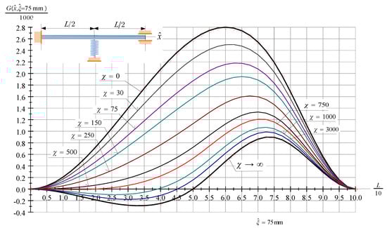
Figure 2. The Green function (the dimensionless vertical displacement field) of an FssF beam subjected to a dimensionless unit force at $\xi =0.75$.

3.2. Green Function for FssP Beams

Repeating the calculation steps presented in Section 3.1 but now for FssP beams yields the elements of the Green function (the calculation steps are omitted):

$$\begin{array}{cc}\hfill & G_{1I}(x,\xi )=\sum _{\ell =1}^4\left(a_{\ell I}\left(\xi \right)\pm b_{\ell I}\left(\xi \right)\right)w_{\ell }\left(x\right)=\left(-\frac{{\xi }^3}{12}\pm \frac{{\xi }^3}{12}\right)+\left(\frac{3\xi }{12}\pm \left(-\frac{3{\xi }^2}{12}\right)\right)x+\hfill \\ \hfill & +\left(\frac{3}{12}\xi \frac{12\ell \left({\ell }^2+{\xi }^2-3\xi \ell \right)-\chi b{\left(b-\ell \right)}^2\left(b^3-4b^2\ell -2{\xi }^{2}b+12b\ell \xi -4\ell {\xi }^2\right)}{\chi b^3\left(4\ell -b\right){\left(b-\ell \right)}^2+12{\ell }^3}\pm \frac{3\xi }{12}\right)x^2+\hfill \\ \hfill & +(\frac{1}{12}\frac{12{\xi }^2\left(3\ell -\xi \right)-12{\ell }^3}{\chi b^3\left(4\ell -b\right){\left(b-\ell \right)}^2+12{\ell }^3}+\hfill \\ \hfill & +\frac{1}{12}\frac{\chi {\left(b-\ell \right)}^2\left(b^4-4b^3\ell +6b^2{\xi }^2-8{\xi }^{3}b+12{\xi }^{2}b\ell -4{\xi }^3\ell \right)}{\chi b^3\left(4\ell -b\right){\left(b-\ell \right)}^2+12{\ell }^3}\pm \frac{-1}{12})x^3,\hfill \end{array}$$

(54)

$$\begin{array}{c}{G}_{2I}(x,\xi )=\sum _{m=1}^4{c}_{mI}\left(\xi \right)w_m\left(x\right)=\frac{1}{2}\left(\ell -x\right){\xi }^2(\frac{2\left(6x{\ell }^2-2{\ell }^2\xi -3x^2\ell -2\ell \xi x+\xi x^2\right)}{\chi b^3\left(4\ell -b\right){\left(\ell -b\right)}^2+12{\ell }^3}+\hfill \\ \hfill +\frac{\chi b^2\left(b-x\right)\left(\ell -b\right)\left(2\ell -b-x\right)\left(b-\xi \right)}{\chi b^3\left(4\ell -b\right){\left(\ell -b\right)}^2+12{\ell }^3}),\end{array}$$

(55)

$$\begin{array}{c}{G}_{1II}(x,\xi )=\sum _{m=1}^4{c}_{mII}\left(\xi \right)w_m\left(x\right)=\frac{1}{2}\left(\ell -\xi \right)x^2(\frac{2\left(6\xi {\ell }^2-2{\ell }^{2}x-3{\xi }^2\ell -2\ell x\xi +x{\xi }^2\right)}{\chi b^3\left(4\ell -b\right){\left(\ell -b\right)}^2+12{\ell }^3}+\hfill \\ \hfill +\frac{\chi b^2\left(b-\xi \right)\left(\ell -b\right)\left(2\ell -b-\xi \right)\left(b-x\right)}{\chi b^3\left(4\ell -b\right){\left(\ell -b\right)}^2+12{\ell }^3}),\end{array}$$

(56)

$$\begin{array}{cc}\hfill & G{}_{2II}(x,\xi )=\sum _{\ell =1}^4\left(a_{\ell II}\left(\xi \right)\pm b_{\ell II}\left(\xi \right)\right)w_{\ell }\left(x\right)=\hfill \\ \hfill & =-\frac{1}{12}\frac{12{\ell }^3{\xi }^3+\chi b^3\left(b^3{\xi }^3-9b{\ell }^2{\xi }^3-6b^3{\xi }^2\ell -12b^2\xi {\ell }^3+4{\ell }^3{\xi }^3+18b^2{\ell }^2{\xi }^2+4b^3{\ell }^3\right)}{\chi b^3\left(4\ell -b\right){\left(\ell -b\right)}^2+12{\ell }^3}\pm \frac{{\xi }^3}{12}+\hfill \\ \hfill & +\left(\frac{3}{12}\frac{12{\ell }^3{\xi }^2+\chi b^3\left(4b^2{\ell }^3-12b\xi {\ell }^3+4{\ell }^3{\xi }^2+9b{\ell }^2{\xi }^2+2b^2{\xi }^3-b^3{\xi }^2-6b\ell {\xi }^3\right)}{\chi b^3\left(4\ell -b\right){\left(\ell -b\right)}^2+12{\ell }^3}\pm \frac{-3{\xi }^2}{12}\right)x+\hfill \\ \hfill & +(\frac{3}{12}\frac{12\ell \xi \left({\xi }^2-3\ell \xi +{\ell }^2\right)}{\chi b^3\left(4\ell -b\right){\left(\ell -b\right)}^2+12{\ell }^3}+\hfill \\ \hfill & +\frac{3}{12}\frac{\chi b^3\left(9b\xi {\ell }^2-12{\ell }^2{\xi }^2+4\ell {\xi }^3+2b^3\ell -b^3\xi +4\xi {\ell }^3-6b^2{\ell }^2\right)}{\chi b^3\left(4\ell -b\right){\left(\ell -b\right)}^2+12{\ell }^3}\pm \frac{3\xi }{12})x^2+\hfill \\ \hfill & +(-\frac{1}{12}\frac{12\left({\xi }^3-3\ell {\xi }^2+{\ell }^3\right)}{\chi b^3\left(4\ell -b\right){\left(\ell -b\right)}^2+12{\ell }^3}-\hfill \\ \hfill & -\frac{1}{12}\frac{\chi b^3\left(4{\ell }^3-9b{\ell }^2+18b\xi \ell -12{\xi }^2\ell -6b^2\xi +4{\xi }^3+b^3\right)}{\chi b^3\left(4\ell -b\right){\left(\ell -b\right)}^2+12{\ell }^3}\pm \frac{-1}{12})x^3.\hfill \end{array}$$

(57)

Figure 3 shows the Green function of an FssP beam under the same conditions as Figure 2 depicts the Green function of an FssF beam. If ($\chi =0$) [$\chi \to \infty$] the beam behaves as if it were (a fixed-pinned beam) [an FrP beam].

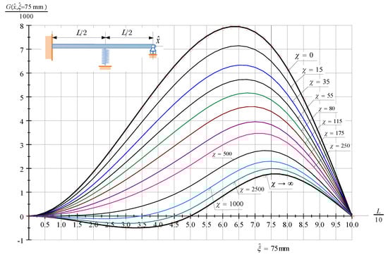
Figure 3. The Green function (the dimensionless vertical displacement field) of an FssP beam subjected to a dimensionless unit force at $\xi =0.75$.

3.3. Green Function for PssP Beams

As regards PssP beams, the following equations provide the elements of the Green function (the calculation steps are again omitted):

$$\begin{array}{c}{G}_{1I}(x,\xi )=\sum _{\ell =1}^4\left(a_{\ell I}\left(\xi \right)\pm b_{\ell I}\left(\xi \right)\right)w_{\ell }\left(x\right)=\left(-\frac{{\xi }^3}{12}\pm \frac{{\xi }^3}{12}\right)+\hfill \\ \hspace{1em}\hspace{1em}\hspace{1em}\hspace{1em}\hspace{1em} +\left(\frac{1}{12}\xi \frac{12{\ell }^3+6{\xi }^2\ell -9{\ell }^2\xi +\chi b{\left(\ell -b\right)}^2\left(4b^2\ell -3b\ell \xi +2{\xi }^2\ell +{\xi }^{2}b-b^3\right)}{\ell \left(\chi b^2{\left(\ell -b\right)}^2+3\ell \right)}\pm \left(-\frac{3{\xi }^2}{12}\right)\right)x+\\ \hspace{1em}\hspace{1em}\hspace{1em}\hspace{1em}\hspace{1em}\hspace{1em}\hspace{1em}\hspace{1em}\hspace{1em}\hspace{1em}\hspace{1em}\hspace{1em}\hspace{1em}\hspace{1em} +\left(-\frac{3\xi }{12}\pm \frac{3\xi }{12}\right)x^2+\left(-\frac{1}{12}\frac{3{\ell }^2-6\ell \xi +\chi {\left(\ell -b\right)}^2\left(b^2\ell -2b\ell \xi -\xi b^2+{\xi }^3\right)}{\ell \left(\chi b^2{\left(\ell -b\right)}^2+3\ell \right)}\pm \frac{-1}{12}\right)x^3,\hfill \end{array}$$

(58)

$$\begin{array}{c}{G}_{2I}(x,\xi )=\sum _{\ell =1}^4{c}_{\ell I}\left(\xi \right)w_{\ell }\left(x\right)=\frac{\xi }{12}\frac{1}{\ell \left(\chi b^2{\left(\ell -b\right)}^2+3\ell \right)}(6\ell \left(\ell -x\right)\left(2x\ell -x^2-{\xi }^2\right)+\hfill \\ \hfill +\chi b\left(b-x\right)\left(\ell -x\right)\left(\ell -b\right)\left(2\ell -b-x\right)\left(b^2-{\xi }^2\right)),\end{array}$$

(59)

$$\begin{array}{c}{G}_{1II}(x,\xi )=\sum _{\ell =1}^4{c}_{\ell II}\left(\xi \right)w_{\ell }\left(x\right)=\frac{x}{12}\frac{1}{\ell \left(\chi b^2{\left(\ell -b\right)}^2+3\ell \right)}(6\ell \left(\ell -\xi \right)\left(2\xi \ell -{\xi }^2-x^2\right)+\hfill \\ \hfill +\chi b\left(b-\xi \right)\left(\ell -\xi \right)\left(\ell -b\right)\left(2\ell -b-\xi \right)\left(b^2-x^2\right))\end{array}$$

(60)

$$\begin{array}{cc}\hfill G& {}_{2II}(x,\xi )=\sum _{\ell =1}^4\left(a_{\ell II}\left(\xi \right)\pm b_{\ell II}\left(\xi \right)\right)w_{\ell }\left(x\right)=\hfill \\ \hfill & =-\frac{1}{12}\frac{3\ell {\xi }^3-\chi b^2\left(2b^2{\ell }^2\xi -{\ell }^2{\xi }^3-3\ell b^2{\xi }^2+2b\ell {\xi }^3-\ell b^4+b^4\xi \right)}{\chi b^2{\left(\ell -b\right)}^2+3\ell }\pm \frac{{\xi }^3}{12}+\hfill \\ \hfill & +(\frac{1}{12}\frac{3\ell \xi \left(2{\xi }^2-3\ell \xi +4{\ell }^2\right)}{\ell \left(\chi b^2{\left(\ell -b\right)}^2+3\ell \right)}+\hfill \\ \hfill & +\frac{1}{12}\frac{\chi b^2\left(3{\ell }^3{\xi }^2-8b{\ell }^3\xi +2{\ell }^3{b}^2+6b{\xi }^2{\ell }^2-4b\ell {\xi }^3+\ell b^4-b^4\xi +b^2{\xi }^3\right)}{\ell \left(\chi b^2{\left(\ell -b\right)}^2+3\ell \right)}\pm \frac{-3{\xi }^2}{12})x+\hfill \\ \hfill & +\left(\frac{3}{12}\frac{-3\ell \xi +\chi b^2\left({\xi }^3+2b\xi \ell -3{\xi }^2\ell +\xi {\ell }^2-b^2\ell \right)}{\chi b^2{\left(\ell -b\right)}^2+3\ell }\pm \frac{3\xi }{12}\right)x^2+\hfill \\ \hfill & +\left(-\frac{1}{12}\frac{3{\ell }^2-6\ell \xi +\chi b^2\left(-b^2\xi +{\xi }^3+{\ell }^3-2b{\ell }^2+4b\xi \ell -3{\xi }^2\ell \right)}{\ell \left(\chi b^2{\left(\ell -b\right)}^2+3\ell \right)}\pm \frac{-1}{12}\right)x^3.\hfill \end{array}$$

(61)

Figure 4 depicts the Green function of pinned-pinned beams with an intermediate spring support. If ($\chi =0$)[$\chi \to \infty$] the beam behaves as if it were (a pinned-pinned beam) [a PrP beam].

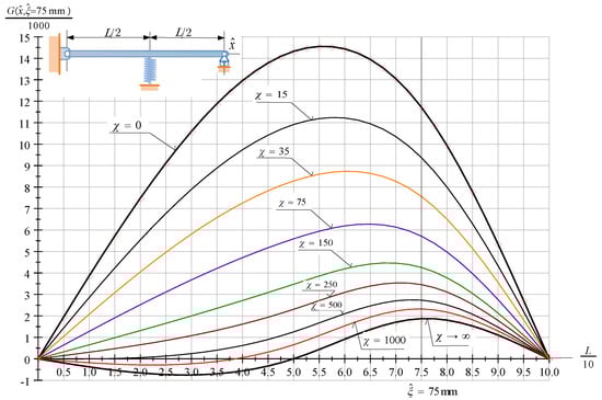
Figure 4. The Green function (the dimensionless vertical displacement field) of a PssP beam subjected to a dimensionless unit force at $\xi =0.75$.

It is worthy of mention that the three BVPs for which we have determined the Green functions are all self-adjoint. Hence, the Green functions given by Equations (40), (41), (52) and (53) (FssF beams), (54)–(57) (FssP beams), (58)–(61) (PssP beams) satisfy the symmetry condition $G(x,\xi )=G(\xi ,\xi )$

The Green functions (40), (41), (52) and (53) (FssF beams), (54)–(57) (FssP beams), (58)–(61) (PssP beams) are dimensionless quantities. However, if we write $\widehat{b}$, L, $\widehat{x}$, $\widehat{\xi }$ and $\widehat{\chi }$ for b, ℓ, x, $\xi$ and $\chi$ in these equations we obtain the Green function for the case of a selected length unit. Then the unit of the Green function will coincide with the cube of the length unit selected and the displacement field $\widehat{w}\left(\widehat{x}\right)$ due to the distributed load $f_z\left(\widehat{x}\right)$ can be given in a closed form:

$$\widehat{w}\left(\widehat{x}\right)=\frac{1}{I_{ey}}{\int }_0^{L}G(\widehat{x},\widehat{\xi })f_z\left(\widehat{\xi }\right)\mathrm{d}\xi .$$

(62)

Assume that $\chi \to \infty$. Then the limit values of the Green functions given by Equations (40), (41), (52) and (53) (FssF beams), (54)–(57) (FssP beams), (58)–(61) (PssP beams) coincide with the Green functions given by Equations (3.22) (3.23) (FrF beams), (3.30), (3.31) (FrP beams) in [32] and (64), (65), (74), (75) (PrP beams) in [34].

These limit values are presented in Appendix A as well.

It is also worthy of mention that Figure 2, Figure 3 and Figure 4 depict the deformed E-weighted centerline of the beams considered due to a dimensionless and vertical unit load $f_z$—see Equation (5)—applied to the beams at the point $\xi$. For $\chi \to \infty$ the curves representing the Green functions in Figure 2, Figure 3 and Figure 4 coincide, obviously, with those curves presented in [32] for FrF, FrP and PrP beams.

4. The Stability Problem of FssF, SssP and PssP Beams with Three Supports

4.1. Solution Procedures

The critical loads are found numerically by solving the eigenvalue problem determined by the homogeneous Fredholm integral Equation (11) with the boundary element technique based on the procedure presented in [35]—see Subsection 8.12.5 for details in the book cited. The beam was subdivided into 40 quadratic elements in the developed Fortran 90 code. The obtained algebraic eigenvalue problem was solved with tha DGVLRG subroutine of the International Mathematical Science Library.

The kernel in Equation (11) has the form

$$\mathcal{K}(x,\xi )=\left\{\begin{array}{cc}{\mathcal{K}}_{1I}(x,\xi )\hfill & \mathrm{if}x,\xi \in [0,b],\hfill \\ {\mathcal{K}}_{2I}(x,\xi )\hfill & \mathrm{if}x\in [b,\ell ]\mathrm{and}\xi \in [0,b],\hfill \\ {\mathcal{K}}_{1II}(x,\xi )\hfill & \mathrm{if}x\in [0,b]\mathrm{and}\xi \in [b,\ell ],\hfill \\ {\mathcal{K}}_{2II}(x,\xi )\hfill & \mathrm{if}x,\xi \in [b,\ell ],\hfill \end{array}\right.$$

(63)

where

$$\begin{array}{cccc}\hfill {\mathcal{K}}_{1I}(x,\xi )& =\frac{{\partial }^2{G}_{1I}(x,\xi )}{\partial x\partial \xi },\hfill & \hfill {\mathcal{K}}_{2I}(x,\xi )& =\frac{{\partial }^2{G}_{2I}(x,\xi )}{\partial x\partial \xi },\hfill \\ \hfill {\mathcal{K}}_{1II}(x,\xi )& =\frac{{\partial }^2{G}_{1II}(x,\xi )}{\partial x\partial \xi },\hfill & \hfill {\mathcal{K}}_{2II}(x,\xi )& =\frac{{\partial }^2{G}_{2II}(x,\xi )}{\partial x\partial \xi }.\hfill \end{array}$$

(64)

4.2. The Kernel for FssF Beams

Making use of Equations (40), (41), (52), (53), (63) and (64) we obtain the elements of the kernel function for FssF beams in the following form:

$$\begin{array}{c}{\mathcal{K}}_{1I}(x,\xi )=\frac{{\partial }^2{G}_{1I}(x,\xi )}{\partial x\partial \xi }=\left(\frac{\xi }{2}\pm \left(-\frac{\xi }{2}\right)\right)+\hfill \\ +\left(\frac{1}{2}\frac{3{\ell }^2\left(6{\xi }^2-8\xi \ell +{\ell }^2\right)+\chi b{\left(\ell -b\right)}^3\left(b^2\ell -2b^2\xi +3b{\xi }^2-6\ell b\xi +3\ell {\xi }^2\right)}{\ell \left(\chi b^3{\left(\ell -b\right)}^3+3{\ell }^3\right)}\pm \frac{1}{2}\right)x+\\ \hspace{1em}\hspace{1em}\hspace{1em}\hspace{1em}\hspace{1em}\hspace{1em}\hspace{1em}\hspace{1em}\hspace{1em}\hspace{1em}\hspace{1em}\hspace{1em}\hspace{1em}\hspace{1em}\hspace{1em}\hspace{1em}\hspace{1em}+\left(\frac{1}{4}\frac{36\xi \ell \left(\ell -\xi \right)+\chi {\left(\ell -b\right)}^3\left(6b^2\xi -9b{\xi }^2+6\ell b\xi -3\ell {\xi }^2\right)}{\ell \left(\chi b^3{\left(\ell -b\right)}^3+3{\ell }^3\right)}{x}^2\right),\hfill \end{array}$$

(65)

$$\begin{array}{c}{\mathcal{K}}_{2I}(x,\xi )=\frac{{\partial }^2{G}_{2I}(x,\xi )}{\partial x\partial \xi }=\hfill \\ \hspace{1em}=-\frac{12\ell \xi \left(x-\ell \right)\left({\ell }^2-3x\ell +3x\xi \right)+\chi b^2{\left(\ell -b\right)}^2\xi \left(2b-3\xi \right)\left(\ell -x\right)\left(2b-3x+\ell \right)}{4\ell \left(\chi b^3{\left(\ell -b\right)}^3+3{\ell }^3\right)},\hfill \end{array}$$

(66)

$$\begin{array}{c}{\mathcal{K}}_{1II}(x,\xi )=\frac{{\partial }^2{G}_{1II}(x,\xi )}{\partial x\partial \xi }=\hfill \\ \hspace{1em}=-\frac{12x\ell \left(\xi -\ell \right)\left(3x\xi -3\xi \ell +{\ell }^2\right)+\chi b^2{\left(\ell -b\right)}^{2}x\left(2b-3x\right)\left(\ell -\xi \right)\left(2b-3\xi +\ell \right)}{4\ell \left(\chi b^3{\left(\ell -b\right)}^3+3{\ell }^3\right)},\hfill \end{array}$$

(67)

$$\begin{array}{cc}\hfill & \mathcal{K}{}_{2II}(x,\xi )=\frac{{\partial }^2{G}_{2II}(x,\xi )}{\partial x\partial \xi }=\hfill \\ \hfill & =\frac{1}{4}\frac{6{\ell }^3\xi +\chi b^3\left(6b^2{\xi }^2-2b^3\xi -9b{\xi }^2\ell +6b\xi {\ell }^2-3b{\ell }^3+2\xi {\ell }^3\right)}{\chi b^3{\left(\ell -b\right)}^3+3{\ell }^3}\pm -\frac{\xi }{2}+\hfill \\ \hfill & +\left(\frac{1}{2}\frac{3{\ell }^2\left({\ell }^2-8\xi \ell +6{\xi }^2\right)+\chi b^3\left(2b^3\xi -b^3\ell -3b^2{\xi }^2+3b{\ell }^3+6{\xi }^2{\ell }^2-8\xi {\ell }^3+{\ell }^4\right)}{\ell \left(\chi b^3{\left(\ell -b\right)}^3+3{\ell }^3\right)}\pm \frac{1}{2}\right)x-\hfill \\ \hfill & -\frac{3}{4}\frac{12\xi \ell \left(\xi -\ell \right)+\chi b^3\left(\xi -\ell \right)\left(4\xi \ell -3b\ell -3b\xi +2b^2\right)}{\ell \left(\chi b^3{\left(\ell -b\right)}^3+3{\ell }^3\right)}{x}^2.\hfill \end{array}$$

(68)

Figure 5 represents the kernel function of an FssF beam for various values of $\chi$ if $\widehat{b}=L/2$ and $\xi =0.75$.

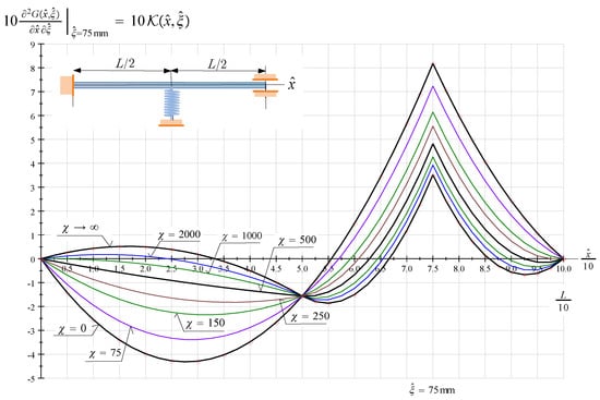
Figure 5. The kernel function of an FssF beam against $x=\widehat{x}/L$; $\chi$ is a parameter and $\xi =0.75$.

4.3. The Kernel for FssP Beams

A comparison of Equations (54)–(57), (63) and (64) yields the elements of the kernel function for FssP beams:

$$\begin{array}{c}{\mathcal{K}}_{1I}(x,\xi )=\frac{{\partial }^2{G}_{1I}(x,\xi )}{\partial x\partial \xi }=\left(\frac{\xi }{2}\pm \left(-\frac{\xi }{2}\right)\right)+\hfill \\ \hspace{1em}\hspace{1em}\hspace{1em}\hspace{1em}\hspace{1em}\hspace{1em}+\left(-\frac{1}{2}\frac{\chi b{\left(\ell -b\right)}^2\left(b^3-4\ell b^2-6b{\xi }^2+24\ell b\xi -12\ell {\xi }^2\right)-12\ell \left(3{\xi }^2-6\xi \ell +{\ell }^2\right)}{\chi b^3\left(4\ell -b\right){\left(b-\ell \right)}^2+12{\ell }^3}\pm \frac{1}{2}\right)x+\\ \hfill +\left(\frac{1}{4}\frac{12\chi \xi {\left(\ell -b\right)}^2\left(2b\ell -2b\xi -\xi \ell +b^2\right)-36\xi \left(\xi -2\ell \right)}{\chi b^3\left(4\ell -b\right){\left(b-\ell \right)}^2+12{\ell }^3}{x}^2\right),\end{array}$$

(69)

$$\begin{array}{c}{\mathcal{K}}_{2I}(x,\xi )=\frac{{\partial }^2{G}_{2I}(x,\xi )}{\partial x\partial \xi }=\hfill \\ \hfill =\frac{1}{2}\frac{\chi b^2\xi \left(2b-3\xi \right)\left(b-\ell \right)\left(-b^2+2b\ell +3x^2-6x\ell +2{\ell }^2\right)+6\xi \left(4{\ell }^3-3x\left(\xi -2\ell \right)\left(x-2\ell \right)\right)}{\chi b^3\left(4\ell -b\right){\left(b-\ell \right)}^2+12{\ell }^3},\end{array}$$

(70)

$$\begin{array}{c}{\mathcal{K}}_{1II}(x,\xi )=\frac{{\partial }^2{G}_{1II}(x,\xi )}{\partial x\partial \xi }=\hfill \\ \hfill =\frac{1}{2}\frac{\chi b^{2}x\left(2b-3x\right)\left(b-\ell \right)\left(-b^2+2b\ell +3{\xi }^2-6\xi \ell +2{\ell }^2\right)+6x\left(4{\ell }^3-3\xi \left(\xi -2\ell \right)\left(x-2\ell \right)\right)}{\chi b^3\left(4\ell -b\right){\left(\ell -b\right)}^2+12{\ell }^3},\end{array}$$

(71)

$$\begin{array}{cc}\hfill & \mathcal{K}{}_{2II}(x,\xi )=\frac{{\partial }^2{G}_{2II}(x,\xi )}{\partial x\partial \xi }=\hfill \\ \hfill & =\frac{1}{4}\frac{b^3\chi \left(-2b^3\xi +6b^2\xi -18b{\xi }^2\ell +18b\xi {\ell }^2-12b{\ell }^3+8\xi {\ell }^3\right)+24{\ell }^3\xi }{\chi b^3\left(4\ell -b\right){\left(\ell -b\right)}^2+12{\ell }^3}\pm \frac{-1}{2}\xi +\hfill \\ \hfill & +\left(\frac{1}{2}\frac{\chi b^3\left(-b^3+9b{\ell }^2+12{\xi }^2\ell -24\xi {\ell }^2+4{\ell }^3\right)+12\ell \left(3{\xi }^2-6\xi \ell +{\ell }^2\right)}{\chi b^3\left(4\ell -b\right){\left(\ell -b\right)}^2+12{\ell }^3}\pm \frac{1}{2}\right)x+\hfill \\ \hfill & +\left(-\frac{3}{12}\frac{\chi b^3\left(6b^2-18\ell b-12{\xi }^2+24\ell \xi \right)-36\xi \left(\xi -2\ell \right)}{\chi b^3\left(4\ell -b\right){\left(\ell -b\right)}^2+12{\ell }^3}\right)x^2.\hfill \end{array}$$

(72)

Figure 6 depicts the kernel function of an FssP beam for various values of $\chi$ if $\widehat{b}=L/2$ and $\xi =0.75$.

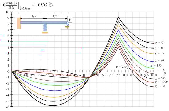
Figure 6. The kernel function of an FssP beam against $x=\widehat{x}/L$; $\chi$ is a parameter and $\xi =0.75$.

4.4. The Kernel for PssP Beams

Utilizing Equations (58)–(61), (63) and (64), it can be checked that the elements of the kernel function for PssP beams assume the following forms:

$$\begin{array}{c}{\mathcal{K}}_{1I}(x,\xi )=\frac{{\partial }^2{G}_{1I}(x,\xi )}{\partial x\partial \xi }=\hfill \\ \hspace{1em}=\left(\frac{1}{12}\frac{\chi b{\left(\ell -b\right)}^2\left(6{\xi }^2\ell -6b\ell \xi +4b^2\ell -b^3+3{\xi }^{2}b\right)+6\ell \left(2{\ell }^2+3{\xi }^2-3\xi \ell \right)}{\ell \left(3\ell +\chi b^2{\left(\ell -b\right)}^2\right)}\pm \left(-\frac{6\xi }{12}\right)\right)+\\ \hspace{1em}\hspace{1em}\hspace{1em}\hspace{1em}\hspace{1em}\hspace{1em}\hspace{1em}\hspace{1em}\hspace{1em}\hspace{1em}\hspace{1em}\hspace{1em}\hspace{1em}\hspace{1em}\hspace{1em}\hspace{1em}\hspace{1em}\hspace{1em} +\left(-\frac{6}{12}\pm \frac{6}{12}\right)x+\left(-\frac{3}{12}\frac{-6\ell +\chi {\left(\ell -b\right)}^2\left(-2b\ell -b^2+3{\xi }^2\right)}{\ell \left(3\ell +\chi b^2{\left(\ell -b\right)}^2\right)}\right)x^2,\hfill \end{array}$$

(73)

$$\begin{array}{c}{\mathcal{K}}_{2I}(x,\xi )=\frac{{\partial }^2{G}_{2I}(x,\xi )}{\partial x\partial \xi }=\hfill \\ \hspace{1em}\hspace{1em} =\frac{1}{12\ell \left(3\ell +\chi b^2{\left(\ell -b\right)}^2\right)}(6\ell \left(3x^2-6x\ell +3{\xi }^2+2{\ell }^2\right)+\\ \hspace{1em}\hspace{1em}\hspace{1em}\hspace{1em}\hspace{1em}\hspace{1em}\hspace{1em}\hspace{1em}\hspace{1em}\hspace{1em} +\chi b\left(\ell -b\right)\left(2{\ell }^2-6x\ell +2b\ell -b^2+3x^2\right)\left(3{\xi }^2-b^2\right)),\hfill \end{array}$$

(74)

$$\begin{array}{c}{\mathcal{K}}_{1II}(x,\xi )=\frac{{\partial }^2{G}_{1II}(x,\xi )}{\partial x\partial \xi }=\hfill \\ \hspace{1em}\hspace{1em} =\frac{1}{12\ell \left(\chi b^2{\left(\ell -b\right)}^2+3\ell \right)}(6\ell \left(3{\xi }^2-6\xi \ell +3x^2+2{\ell }^2\right)+\\ \hspace{1em}\hspace{1em}\hspace{1em}\hspace{1em}\hspace{1em}\hspace{1em}\hspace{1em}\hspace{1em}\hspace{1em}\hspace{1em} +\chi b\left(\ell -b\right)\left(2{\ell }^2-6\xi \ell +2b\ell -b^2+3{\xi }^2\right)\left(3x^2-b^2\right)),\hfill \end{array}$$

(75)

$$\begin{array}{c}\mathcal{K}{}_{2II}(x,\xi )=\frac{{\partial }^2{G}_{2II}(x,\xi )}{\partial x\partial \xi }=\hfill \\ =\frac{1}{12\ell \left(\chi b^2{\left(\ell -b\right)}^2+3\ell \right)}(3\ell \left(6{\xi }^2-6\xi \ell +4{\ell }^2\right)+\\ \hspace{1em}\hspace{1em} +\chi b^2\left(-b^4+3b^2{\xi }^2-12{\xi }^2\ell b+12{\ell }^2\xi b-8{\ell }^{3}b+6{\ell }^3\xi \right))\pm \frac{-6\xi }{12}+\\ \left(\frac{6}{12}\frac{-3\ell +\chi b^2\left(3{\xi }^2+2b\ell -6\xi \ell +{\ell }^2\right)}{\chi b^2{\left(\ell -b\right)}^2+3\ell }\pm \frac{6}{12}\right)x+\\ \hspace{1em}\hspace{1em}\hspace{1em}\hspace{1em}\hspace{1em}\hspace{1em}\hspace{1em}\hspace{1em}\hspace{1em}\hspace{1em} +\left(-\frac{3}{12}\frac{-6\ell +\chi b^2\left(-b^2+4b\ell +3{\xi }^2-6\xi \ell \right)}{\ell \left(\chi b^2{\left(\ell -b\right)}^2+3\ell \right)}\right)x^2.\hfill \end{array}$$

(76)

Figure 7 shows the kernel function of a PssP beam for various values of $\chi$ if $\widehat{b}=L/2$ and $\xi =0.75$.

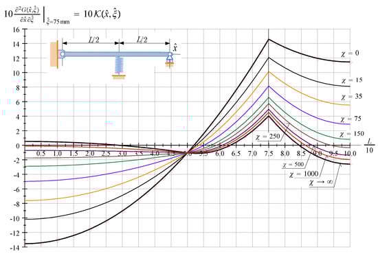
Figure 7. The kernel function of a PssP beam against $x=\widehat{x}/L$; $\chi$ is a parameter and $\xi =0.75$.

The kernel functions given by (65)–(68) (FssF beams), (69)–(72) (FssP beams), (73)–(76) (PssP beams) satisfy the symmetry condition $\mathcal{K}(x,\xi )=\mathcal{K}(\xi ,x)$.

Assume that $\chi \to \infty$. Then, the limit values of the kernel functions given by (65)–(68) (FssF beams), (69)–(72) (FssP beams), (73)–(76) (PssP beams) coincide with the kernel functions given by Equations (4.2) (FrF beams), (4.5) (FrP beams) and (4.7) in [32].

These limit values are also presented in Appendix A.

For $\chi \to \infty$ the curves representing the kernel functions in Figure 5, Figure 6 and Figure 7 coincide, obviously, with those curves presented in [32] for the kernel functions of FrF, FrP and PrP beams.

5. Computational Results

5.1. FssF Beams

Table 2 and Table 3 contain the values of the dimensionless critical force $\sqrt{{\mathcal{N}}_{\mathrm{crit}}}/\pi$ as a function of b. The dimensionless spring constant $\chi$ is a parameter. For symmetry reasons it is sufficient to present the results obtained for $b\in [0,0.5]$.

Table 2. The critical forces of FssF beams if $\chi =25,\dots ,125$.

$\sqrt{{\mathcal{N}}_{\mathbf{crit}}}/\mathit{\pi }$
$\mathit{b}$	$\mathbf{\chi }=\mathbf{25}$	$\mathbf{\chi }=\mathbf{50}$	$\mathbf{\chi }=\mathbf{75}$	$\mathbf{\chi }=\mathbf{100}$	$\mathbf{\chi }=\mathbf{125}$
0.0000	2.000000	2.000000	2.000000	2.000000	2.000000
0.0250	2.000008	2.000013	2.000018	2.000023	2.000028
0.0500	2.000080	2.000157	2.000233	2.000310	2.000386
0.0750	2.000383	2.000761	2.001136	2.001509	2.001880
0.1000	2.001166	2.002313	2.003444	2.004561	2.005663
0.1250	2.002723	2.005379	2.007972	2.010506	2.012982
0.1500	2.005355	2.010514	2.015489	2.020289	2.024922
0.1750	2.009325	2.018181	2.026601	2.034609	2.042232
0.2000	2.014822	2.028690	2.041678	2.053850	2.065267
0.2250	2.021935	2.042170	2.060845	2.078091	2.094027
0.2500	2.030643	2.058561	2.083989	2.107147	2.128241
0.2750	2.040804	2.077623	2.110792	2.140630	2.167450
0.3000	2.052156	2.098938	2.140749	2.177991	2.211072
0.3250	2.064324	2.121912	2.173171	2.218522	2.258424
0.3500	2.076823	2.145766	2.207159	2.261337	2.308701
0.3750	2.089075	2.169522	2.241546	2.305276	2.360891
0.4000	2.100433	2.191993	2.274805	2.348745	2.413589
0.4250	2.110217	2.211797	2.304954	2.389443	2.464612
0.4500	2.117777	2.227448	2.329532	2.424019	2.510233
0.4750	2.122562	2.237538	2.345833	2.447969	2.543998
0.5000	2.124201	2.241031	2.351573	2.456659	2.556943

Table 3. The critical forces of FssF beams if $\chi =150,\dots ,1500$ and $\chi \to \infty$.

$\sqrt{{\mathcal{N}}_{\mathbf{crit}}}/\mathit{\pi }$
$\mathbf{b}$	$\mathit{\chi }=\mathbf{150}$	$\mathbf{\chi }=\mathbf{200}$	$\mathbf{\chi }=\mathbf{325}$	$\mathbf{\chi }=\mathbf{500}$	$\mathbf{\chi }=\mathbf{1500}$	$\mathbf{\chi }\to \infty$
0.0000	2.000000	2.000000	2.000000	2.000000	2.000000	2.000000
0.0250	2.000033	2.000042	2.000067	2.000100	2.000293	2.038216
0.0500	2.000462	2.000613	2.000990	2.001511	2.004361	2.077889
0.0750	2.002249	2.002979	2.004767	2.007183	2.019289	2.119074
0.1000	2.006750	2.008884	2.013983	2.020605	2.049702	2.161815
0.1250	2.015401	2.020078	2.030899	2.044229	2.094262	2.206145
0.1500	2.029394	2.037888	2.056787	2.078661	2.148228	2.252082
0.1750	2.049491	2.063007	2.091798	2.122924	2.207134	2.299619
0.2000	2.075983	2.095515	2.135248	2.175238	2.268186	2.348715
0.2250	2.108766	2.135051	2.186031	2.233702	2.330019	2.399278
0.2500	2.147465	2.181004	2.242947	2.296665	2.392061	2.451142
0.2750	2.191547	2.232672	2.304889	2.362820	2.454057	2.504040
0.3000	2.240399	2.289358	2.370903	2.431136	2.515766	2.557558
0.3250	2.293366	2.350419	2.440155	2.500707	2.576781	2.611080
0.3500	2.349744	2.415267	2.511842	2.570559	2.636388	2.663708
0.3750	2.408718	2.483339	2.585016	2.639404	2.693437	2.714177
0.4000	2.469216	2.554051	2.658291	2.705314	2.746205	2.760765
0.4250	2.529572	2.626716	2.729274	2.765312	2.792309	2.801259
0.4500	2.586620	2.700418	2.793376	2.814985	2.828768	2.833058
0.4750	2.633089	2.773688	2.841720	2.848596	2.852393	2.853522
0.5000	2.652952	2.833793	2.860604	2.860604	2.860604	2.860604

Figure 8 shows the dimensionless critical force against b. $\chi$ is a parameter. If $\chi =0$ the beam is a fixed-fixed beam for which $\sqrt{{\mathcal{N}}_{\mathrm{crit}}}/\pi =2.000$. It is obvious that the dimensionless critical force has a maximum if $b=0.5$.

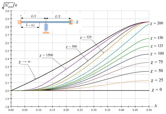
Figure 8. The dimensionless critical force of FssF beams as a function of b; $\chi$ is a parameter.

5.2. FssP Beams

Table 4, Table 5 and Table 6 contain the values of the dimensionless critical force $\sqrt{{\mathcal{N}}_{\mathrm{crit}}}/\pi$ as a function of b. The dimensionless spring constant $\chi$ is a parameter.

Table 4. The critical forces of FssP beams if $\chi =15,\dots ,115$.

$\sqrt{{\mathcal{N}}_{\mathbf{crit}}}/\mathit{\pi }$
$\mathit{b}$	$\mathbf{\chi }=\mathbf{15}$	$\mathbf{\chi }=\mathbf{35}$	$\mathbf{\chi }=\mathbf{55}$	$\mathbf{\chi }=\mathbf{80}$	$\mathbf{\chi }=\mathbf{115}$
0.0000	1.430302	1.430302	1.430302	1.430302	1.430302
0.0500	1.430334	1.430377	1.430420	1.430473	1.430547
0.1000	1.430784	1.431422	1.432052	1.432831	1.433905
0.1500	1.432544	1.435455	1.438280	1.441695	1.446273
0.2000	1.436662	1.444720	1.452328	1.461255	1.472769
0.2500	1.443950	1.460773	1.476177	1.493662	1.515280
0.3000	1.454692	1.484013	1.510111	1.538821	1.572915
0.3500	1.468509	1.513634	1.552947	1.595125	1.643523
0.4000	1.484348	1.547702	1.602312	1.660025	1.724640
0.4500	1.500535	1.583160	1.654563	1.729929	1.813437
0.5000	1.514927	1.615748	1.704260	1.799175	1.905547
0.5500	1.525206	1.640163	1.743538	1.857971	1.991783
0.6000	1.529367	1.651044	1.762835	1.890806	2.050418
0.6500	1.526294	1.645008	1.755043	1.882616	2.046060
0.7000	1.516169	1.622456	1.720727	1.833762	1.975444
0.7500	1.500463	1.587353	1.667434	1.758843	1.871752
0.8000	1.481573	1.545450	1.604616	1.672479	1.757022
0.8500	1.462350	1.502853	1.540969	1.585485	1.642410
0.9000	1.445718	1.465619	1.484801	1.507815	1.538331
0.9500	1.434358	1.439708	1.444994	1.451512	1.460475
0.9750	1.431330	1.432696	1.434058	1.435753	1.438115
0.9800	1.430961	1.431838	1.432713	1.433804	1.435326
0.9900	1.430467	1.430687	1.430907	1.431182	1.431566
0.9975	1.430312	1.430326	1.430340	1.430357	1.430381

Table 5. The critical forces of FssP beams if $\chi =170,\dots ,2500$.

$\sqrt{{\mathcal{N}}_{\mathbf{crit}}}/\mathit{\pi }$
$\mathit{b}$	$\mathbf{\chi }=\mathbf{170}$	$\mathbf{\chi }=\mathbf{250}$	$\mathbf{\chi }=\mathbf{500}$	$\mathbf{\chi }=\mathbf{1000}$	$\mathbf{\chi }=\mathbf{2500}$
0.0000	1.430302	1.430302	1.430302	1.430302	1.43030
0.0500	1.430674	1.430833	1.431353	1.432366	1.43519
0.1000	1.435700	1.437868	1.444538	1.455748	1.47845
0.1500	1.453609	1.461967	1.484671	1.514784	1.55600
0.2000	1.490195	1.508606	1.551816	1.596797	1.64233
0.2500	1.546037	1.576049	1.637247	1.689125	1.73202
0.3000	1.618623	1.659962	1.734342	1.787809	1.82642
0.3500	1.705053	1.756927	1.840447	1.892859	1.92721
0.4000	1.803191	1.865196	1.955048	2.004906	2.03510
0.4500	1.911581	1.984124	2.077841	2.123440	2.14901
0.5000	2.028652	2.113167	2.206504	2.244631	2.26416
0.5500	2.150917	2.250231	2.332179	2.357130	2.36848
0.6000	2.266076	2.386936	2.429884	2.437159	2.44005
0.6500	2.293059	2.452225	2.457446	2.457895	2.45806
0.7000	2.172303	2.316725	2.402885	2.418421	2.42438
0.7500	2.026359	2.154562	2.296332	2.339839	2.35800
0.8000	1.876349	1.986250	2.157401	2.236818	2.27423
0.8500	1.726880	1.812434	1.985291	2.106331	2.17705
0.9000	1.586370	1.639609	1.773783	1.919260	2.04977
0.9500	1.475409	1.493344	1.547757	1.635968	1.79607
0.9750	1.442131	1.447093	1.463185	1.493419	1.57070
0.9800	1.437921	1.441141	1.451681	1.471908	1.52642
0.9900	1.432224	1.433044	1.435766	1.441151	1.45684
0.9975	1.430422	1.430474	1.430646	1.430990	1.43201

Table 6. The critical forces of FssP beams if $\chi =5000,$ …, 500,000 and $\chi \to \infty$.

$\sqrt{{\mathcal{N}}_{\mathbf{crit}}}/\mathit{\pi }$
$\mathit{b}$	$\mathbf{\chi }=\mathbf{5000}$	$\mathbf{\chi }$ = 50,000	$\mathbf{\chi }$ = 500,000	$\mathbf{\chi }\to \infty$
0.0000	1.430302	1.430302	1.430302	1.430302
0.0500	1.439304	1.467133	1.483508	1.486263
0.1000	1.498693	1.539600	1.546449	1.547261
0.1500	1.579860	1.609894	1.613513	1.613924
0.2000	1.662822	1.684347	1.686682	1.686943
0.2500	1.748836	1.765158	1.766854	1.767044
0.3000	1.840403	1.853428	1.854753	1.854900
0.3500	1.939021	1.949752	1.950830	1.950950
0.4000	2.045077	2.053978	2.054864	2.054962
0.4500	2.157153	2.164302	2.165007	2.165085
0.5000	2.270140	2.275295	2.275799	2.275855
0.5500	2.371795	2.374598	2.374870	2.374900
0.6000	2.440857	2.441527	2.441591	2.441598
0.6500	2.458107	2.458144	2.458148	2.458148
0.7000	2.426022	2.427372	2.427501	2.427515
0.7500	2.363057	2.367247	2.367649	2.367693
0.8000	2.284880	2.293734	2.294583	2.294677
0.8500	2.198218	2.215921	2.217618	2.217805
0.9000	2.096723	2.137438	2.141358	2.141792
0.9500	1.909498	2.051914	2.067177	2.068868
0.9750	1.665896	1.969510	2.027310	2.033900
0.9800	1.600374	1.929960	2.016812	2.027035
0.9900	1.481535	1.736193	1.865164	2.013432
0.9975	1.433728	1.463150	1.659478	2.003187

Figure 9 depicts the dimensionless critical force against b. $\chi$ is a parameter. If $\chi =0$ the beam is a fixed-pinned beam for which $\sqrt{{\mathcal{N}}_{\mathrm{crit}}}/\pi =1.43029$. Note that the dimensionless critical for reaches its maximum if $b\in [0.62,0.645]$.

Figure 9. The dimensionless critical force of FssP beams as a function of b; $\chi$ is a parameter.

5.3. PssP Beams

Table 7, Table 8 and Table 9 contain the values of the dimensionless critical force $\sqrt{{\mathcal{N}}_{\mathrm{crit}}}/\pi$ as a function of b. The dimensionless spring constant $\chi$ is a parameter. For symmetry reasons it is sufficient to present the results obtained for $b\in [0,0.5]$.

Table 7. The critical forces of PssP beams if $\chi =15,\dots ,115$.

$\sqrt{{\mathcal{N}}_{\mathbf{crit}}}/\mathit{\pi }$
$\mathit{b}$	$\mathbf{\chi }=\mathbf{15}$	$\mathbf{\chi }=\mathbf{35}$	$\mathbf{\chi }=\mathbf{55}$	$\mathbf{\chi }=\mathbf{80}$	$\mathbf{\chi }=\mathbf{115}$
0.0050	1.000038	1.000089	1.000139	1.000203	1.000291
0.0250	1.000946	1.002203	1.003454	1.005009	1.007171
0.0500	1.003744	1.008664	1.013501	1.019434	1.027537
0.0750	1.008283	1.018999	1.029356	1.041818	1.058417
0.1000	1.014401	1.032695	1.050019	1.070410	1.096801
0.1250	1.021899	1.049184	1.074473	1.103551	1.140070
0.1500	1.030560	1.067907	1.101790	1.139857	1.186254
0.1750	1.040153	1.088335	1.131176	1.178259	1.234011
0.2000	1.050443	1.109986	1.161977	1.217974	1.282501
0.2250	1.061192	1.132414	1.193647	1.258436	1.331245
0.2500	1.072159	1.155206	1.225725	1.299237	1.380002
0.2750	1.083106	1.177960	1.257790	1.340055	1.428676
0.3000	1.093790	1.200274	1.289427	1.380600	1.477247
0.3250	1.103973	1.221726	1.320183	1.420549	1.525707
0.3500	1.113416	1.241869	1.349530	1.459481	1.574002
0.3750	1.121889	1.260218	1.376823	1.496781	1.621959
0.4000	1.129173	1.276257	1.401272	1.531525	1.669148
0.4250	1.135072	1.289461	1.421934	1.562324	1.714591
0.4500	1.139416	1.299330	1.437770	1.587206	1.756046
0.4750	1.142077	1.305442	1.447778	1.603709	1.788296
0.5000	1.142973	1.307513	1.451208	1.609538	1.801390

Table 8. The critical forces of PssP beams if $\chi =150,\dots ,1000$.

$\sqrt{{\mathcal{N}}_{\mathbf{crit}}}/\mathit{\pi }$
$\mathit{b}$	$\mathbf{\chi }=\mathbf{150}$	$\mathbf{\chi }=\mathbf{250}$	$\mathbf{\chi }=\mathbf{500}$	$\mathbf{\chi }=\mathbf{1000}$	$\mathbf{\chi }=\mathbf{2500}$
0.0050	1.000380	1.000632	1.001263	1.002520	1.006254
0.0250	1.009316	1.015351	1.029852	1.056549	1.121698
0.0500	1.035409	1.056708	1.103187	1.174045	1.290759
0.0750	1.074091	1.114340	1.191978	1.286865	1.396462
0.1000	1.120924	1.179364	1.278177	1.375881	1.463389
0.1250	1.172332	1.245932	1.355211	1.445158	1.513286
0.1500	1.225865	1.310985	1.422771	1.501934	1.555706
0.1750	1.280037	1.373333	1.482749	1.551418	1.594801
0.2000	1.334066	1.432842	1.537309	1.596787	1.632513
0.2250	1.387633	1.489886	1.588239	1.639912	1.669810
0.2500	1.440701	1.545030	1.636849	1.681877	1.707165
0.2750	1.493394	1.598853	1.684026	1.723276	1.744759
0.3000	1.545916	1.651863	1.730301	1.764355	1.782554
0.3250	1.598500	1.704442	1.775890	1.805074	1.820303
0.3500	1.651374	1.756798	1.820677	1.845096	1.857524
0.3750	1.704736	1.808878	1.864149	1.883732	1.893431
0.4000	1.758730	1.860203	1.905266	1.919853	1.926867
0.4250	1.813415	1.909478	1.942270	1.951800	1.956240
0.4500	1.868675	1.953769	1.972551	1.977382	1.979566
0.4750	1.923800	1.987051	1.992816	1.994141	1.994726
0.5000	1.966030	2.000000	2.000000	2.000000	2.000000

Table 9. The critical forces of PssP beams if $\chi =5000,\dots$, 500,000 and $\chi \to \infty$.

$\sqrt{{\mathcal{N}}_{\mathbf{crit}}}/\mathit{\pi }$
$\mathit{b}$	$\mathbf{\chi }=\mathbf{5000}$	$\mathbf{\chi }$ = 50,000	$\mathbf{\chi }$ = 500,000	$\mathbf{\chi }\to \infty$
0.0050	1.012356	1.101002	1.337454	1.432062
0.0250	1.196323	1.408628	1.449777	1.454511
0.0500	1.367709	1.467128	1.478710	1.479979
0.0750	1.447720	1.500308	1.505839	1.506440
0.1000	1.497758	1.530319	1.533634	1.533994
0.1250	1.537763	1.560180	1.562432	1.562676
0.1500	1.574108	1.590676	1.592328	1.592507
0.1750	1.609223	1.622078	1.623355	1.623493
0.2000	1.644166	1.654485	1.655507	1.655618
0.2250	1.679429	1.687905	1.688743	1.688833
0.2500	1.715212	1.722274	1.722971	1.723046
0.2750	1.751529	1.757450	1.758033	1.758096
0.3000	1.788237	1.793189	1.793676	1.793729
0.3250	1.825015	1.829106	1.829507	1.829551
0.3500	1.861331	1.864623	1.864946	1.864981
0.3750	1.896371	1.898902	1.899150	1.899176
0.4000	1.928968	1.930770	1.930946	1.930964
0.4250	1.957555	1.958677	1.958786	1.958798
0.4500	1.980206	1.980750	1.980803	1.980809
0.4750	1.994896	1.995041	1.995055	1.995056
0.5000	2.000000	2.000000	2.000000	2.000000

Figure 10 shows the graphs the dimensionless critical force against b. $\chi$ is a parameter. If $\chi =0$ the beam is a pinned-pinned beam for which $\sqrt{{\mathcal{N}}_{\mathrm{crit}}}/\pi =1.0$. The dimensionless critical force reaches its maximum if $b=0.5$.

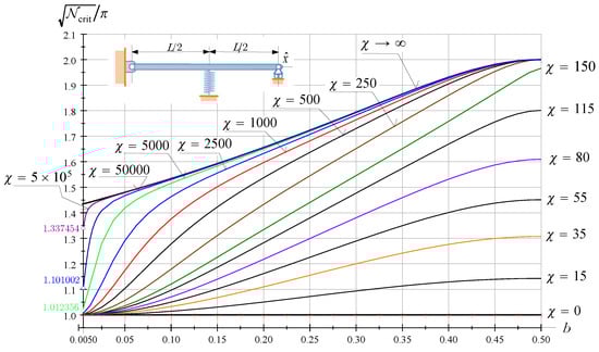
Figure 10. The dimensionless critical force of PssP beams as a function of b; $\chi$ is a parameter.

For $\chi \to \infty$ the curves representing the dimensionless critical forces in Figure 8, Figure 9 and Figure 10 coincide with those curves presented in [32] for the dimensionless critical forces of FrF, FrP and PrP beams.

6. Conclusions

Making use of the definition given in paper [34] we have determined the Green functions for those three point BVPs, which describe the mechanical behavior of fixed-fixed, fixed-pinned and pinned-pinned beams with an intermediate spring support. It is assumed that the beams have cross sectional heterogeneity [33].

With the Green functions the dimensionless displacement field due to the dimensionless distributed forces acting on the E-weighted centerline can be calculated using the formula

$$w\left(x\right)={\int }_0^{\ell =1}G(x,\xi )f\left(\xi \right)d\xi .$$

(77)

The dimensionless bending moment $m\left(x\right)$ is defined by the relation

$$m\left(x\right)=-{\int }_0^{\ell =1}\frac{{\partial }^2}{\partial x^2}G(x,\xi )f\left(\xi \right)d\xi .$$

(78)

If $\chi \to \infty$ the Green functions of FssF, FssP and PssP beams results in the Green functions of FrF, FrP and PrP beams. We remark that these Green functions are presented in Section A.1, Section A.2, Section A.3. See paper [32] for a comparison.

It can be checked that the Green functions of FssF, FssP and PssP beams simplify to the Green functions of fixed-fixed, fixed-pinned and pinned-pinned beams if $\chi =0$ —see Table 8.1 in [35].

Utilizing the Green functions the linear stability problems of these beams are transformed into eigenvalue problems governed by the homogeneous Fredholm integral equation:

$$y\left(x\right)=\mathcal{N}{\int }_0^{\ell =1}\mathcal{K}(x,\xi )y\left(\xi \right)d\xi ,\mathcal{K}(x,\xi )=\frac{{\partial }^{2}G(x,\xi )}{\partial x\partial \xi },y\left(x\right)=\frac{\mathrm{d}w\left(x\right)}{\mathrm{d}x}.$$

(79)

The numerical solution for the eigenvalues of the homogeneous Fredholnm integral equations (for the critical forces) is based on a novel solution procedure published in [35].

The published formalism, the solution procedure that is based on the use of homogeneous Fredholm integral equations with kernels obtained from the Green functions and the numerical results we computed are all valid for beams with cross sectional heterogeneity—these constitute the main novelty in our paper-, however, everything remains valid for homogeneous beams as well provided that $I_{ey}$ is replaced by the product $I_{y}E$, where $I_y$ is the second moment of inertia of the cross section with respect to the axis $\widehat{y}$, while E is the modulus of elasticity.

The numerical results presented in Table 2, Table 3, Table 4, Table 5, Table 6, Table 7, Table 8 and Table 9 for the dimensionless critical force ${\mathcal{N}}_{\mathrm{crit}}$ can be applied in the engineering practice if stability problem should be solved.

If $\chi \to \infty$ the kernel functions of FssF, FssP and PssP beams coincide with the kernel functions of FrF, FrP and PrP beams. These kernel functions are presented in Appendix A.4–Appendix A.6. See paper [32] for a comparison.

For FssP beams the critical force reaches its maximum if $b\in (0.62-0.645)$. The actual value for the optimum location depends on the spring stiffness—see Figure 9.

For completeness Appendix A.7 gives the characteristic equations that provide also the dimensionless critical force.

The eigenvalue problem governed by the integral Equation (79)${}_1$ is transformed into an algebraic eigenvalue problem using the boundary element technique. The solutions for the algebraic eigenvalue problem are compared to the solutions obtained from the numerical solutions of the nonlinear characteristic equations presented in Appendix A.7. The correlation is excellent: the computed values of the dimensionless critical forces agree with each other with four digit accuracy.

Appendix A.1. The Green Function for FrF Beams

Assume that $\chi ⟶\infty$. Then, Equations (40), (41), (52) and (53) (FssF beams) yield

$$\begin{array}{cc}\hfill G_{1I}(x,\xi )& =\frac{1}{12}[\left(-{\xi }^3\pm {\xi }^3\right)+\left(3{\xi }^2\pm \left(-3{\xi }^2\right)\right)x+\hfill \\ \hfill & +\left(\frac{3\xi }{\ell b^2}\left(b^2\ell -3b\ell \xi +\ell {\xi }^2+{\xi }^{2}b-\xi b^2\right)\pm 3\xi \right)x^2+\hfill \\ \hfill & +\left(-\frac{1}{\ell b^3}\left(b^3\ell +\ell {\xi }^3-3b^2{\xi }^2-3b\ell {\xi }^2+3{\xi }^{3}b\right)\pm \left(-1\right)\right)x^3],\hfill \end{array}$$

(A1)

$$G_{2I}(x,\xi )=-\frac{1}{4\ell b\left(\ell -b\right)}{\xi }^2{\left(x-\ell \right)}^2\left(b-x\right)\left(\xi -b\right),$$

(A2)

$$G_{1II}(x,\xi )=-\frac{1}{4\left(\ell -b\right)\ell b}{x}^2{\left(\xi -\ell \right)}^2\left(b-\xi \right)\left(x-b\right),$$

(A3)

$$\begin{array}{c}{G}_{2II}(x,\xi )=-\frac{1}{12}\frac{{\ell }^3{\xi }^3+{\ell }^3{b}^3+b^3{\xi }^3-3b^3{\xi }^2\ell -3b^2{\ell }^3\xi -3b{\ell }^2{\xi }^3+6b^2{\xi }^2{\ell }^2}{{\left(\ell -b\right)}^3}\pm \frac{{\xi }^3}{12}+\hfill \\ +\left(\frac{3}{12}\frac{b^2{\ell }^3+2b^2{\xi }^3+3b{\xi }^2{\ell }^2-3b\ell {\xi }^3+{\ell }^3{\xi }^2-3b{\ell }^3\xi -b^3{\xi }^2}{{\left(\ell -b\right)}^3}\pm \frac{-3{\xi }^2}{12}\right)x+\hfill \\ +\left(\frac{3}{12}\frac{{\ell }^4\xi -4{\ell }^3{\xi }^2+2{\ell }^2{\xi }^3-2b^2{\ell }^3-b^3\ell \xi -b^2{\xi }^3+b^3{\xi }^2+{\ell }^2{b}^3+3b{\ell }^3\xi }{\ell {\left(\ell -b\right)}^3}\pm \frac{3\xi }{12}\right)x^2+\hfill \\ +\left(\frac{1}{12}\frac{3b{\xi }^3-3b^2{\xi }^2+3b{\ell }^3-9b{\ell }^2\xi +6{\xi }^2{\ell }^2-4\ell {\xi }^3+6b^2\xi \ell -b^3\ell -{\ell }^4}{\ell {\left(\ell -b\right)}^3}\pm \frac{-1}{12}\right)x^3.\hfill \end{array}$$

(A4)

These equations provide the Green function for FrF beams.

Appendix A.2. The Green Function for FrP Beams

If $\chi ⟶\infty$, Equations (54)–(57) (FssP beams), yield

$$\begin{array}{cc}\hfill G_{1I}(x,\xi )& =\left(-\frac{1}{12}{\xi }^3\pm \frac{1}{12}{\xi }^3\right)+\left(\frac{3{\xi }^2}{12}\pm \left(-\frac{3{\xi }^2}{12}\right)\right)x+\hfill \\ \hfill & +\left(-\frac{3}{12}\xi \frac{b^3-4b^2\ell -2{\xi }^{2}b+12b\ell \xi -4\ell {\xi }^2}{b^2\left(4\ell -b\right)}\pm \frac{3\xi }{12}\right)x^2+\hfill \\ \hfill & +\left(\frac{1}{12}\frac{b^4-4b^3\ell +6b^2{\xi }^2-8{\xi }^{3}b+12{\xi }^{2}b\ell -4{\xi }^3\ell }{b^3\left(4\ell -b\right)}\pm \frac{-1}{12}\right)x^3,\hfill \end{array}$$

(A5)

$$G_{2I}(x,\xi )=\frac{\left(\ell -x\right){\xi }^2}{2b\left(4\ell -b\right)\left(\ell -b\right)}\left(b-x\right)\left(2\ell -b-x\right)\left(b-\xi \right),$$

(A6)

$$G_{1II}(x,\xi )=\frac{\left(\ell -\xi \right)x^2}{2b\left(4\ell -b\right)\left(\ell -b\right)}\left(b-\xi \right)\left(2\ell -b-\xi \right)\left(b-x\right),$$

(A7)

$$\begin{array}{c}{G}_{2II}(x,\xi )=-\frac{1}{12}\frac{b^3{\xi }^3-9b{\ell }^2{\xi }^3-6b^3{\xi }^2\ell -12b^2\xi {\ell }^3+4{\ell }^3{\xi }^3+18b^2{\ell }^2{\xi }^2+4b^3{\ell }^3}{\left(4\ell -b\right){\left(\ell -b\right)}^2}\pm \frac{{\xi }^3}{12}+\hfill \\ +\left(\frac{3}{12}\frac{4b^2{\ell }^3-12b\xi {\ell }^3+4{\ell }^3{\xi }^2+9b{\ell }^2{\xi }^2+2b^2{\xi }^3-b^3{\xi }^2-6b\ell {\xi }^3}{\left(4\ell -b\right){\left(\ell -b\right)}^2}\pm \frac{-3{\xi }^2}{12}\right)x+\hfill \\ +\left(\frac{3}{12}\frac{9b\xi {\ell }^2-12{\ell }^2{\xi }^2+4\ell {\xi }^3+2b^3\ell -b^3\xi +4\xi {\ell }^3-6b^2{\ell }^2}{\left(4\ell -b\right){\left(\ell -b\right)}^2}\pm \frac{3\xi }{12}\right)x^2+\hfill \\ +\left(-\frac{1}{12}\frac{4{\ell }^3-9b{\ell }^2+18b\xi \ell -12{\xi }^2\ell -6b^2\xi +4{\xi }^3+b^3}{\left(4\ell -b\right){\left(\ell -b\right)}^2}\pm \frac{-1}{12}\right)x^3.\hfill \end{array}$$

(A8)

These equations constitute the Green function for FrP beams.

Appendix A.3. The Green Function for PrP Beams

If $\chi ⟶\infty$, Equations (58)–(61) (PssP beams) results in the following relations:

$$\begin{array}{cc}\hfill G_{1I}(x,\xi )& =\left(-\frac{{\xi }^3}{12}\pm \frac{{\xi }^3}{12}\right)+\left(\frac{1}{12}\xi \frac{4b^2\ell -3b\ell \xi +2{\xi }^2\ell +{\xi }^{2}b-b^3}{b\ell }\pm \left(-\frac{3{\xi }^2}{12}\right)\right)x+\hfill \\ \hfill & +\left(-\frac{3\xi }{12}\pm \frac{3\xi }{12}\right)x^2+\left(-\frac{1}{12}\frac{b^2\ell -2b\ell \xi -\xi b^2+{\xi }^3}{b^2\ell }\pm \frac{-1}{12}\right)x^3,\hfill \end{array}$$

(A9)

$$G_{2I}(x,\xi )=\frac{\xi }{12}\frac{1}{b\ell \left(\ell -b\right)}\left(b-x\right)\left(\ell -x\right)\left(2\ell -b-x\right)\left(b^2-{\xi }^2\right),$$

(A10)

$$G_{1II}(x,\xi )=\frac{x}{12}\frac{1}{b\ell \left(\ell -b\right)}\left(b-\xi \right)\left(\ell -\xi \right)\left(2\ell -b-\xi \right)\left(b^2-x^2\right),$$

(A11)

$$\begin{array}{c}{G}_{2II}(x,\xi )=\frac{1}{12}\frac{2b^2{\ell }^2\xi -{\ell }^2{\xi }^3-3\ell b^2{\xi }^2+2b\ell {\xi }^3-\ell b^4+b^4\xi }{{\left(\ell -b\right)}^2}\pm \frac{{\xi }^3}{12}+\hfill \\ +\left(\frac{1}{12}\frac{3{\ell }^3{\xi }^2-8b{\ell }^3\xi +2{\ell }^3{b}^2+6b{\xi }^2{\ell }^2-4b\ell {\xi }^3+\ell b^4-b^4\xi +b^2{\xi }^3}{\ell {\left(\ell -b\right)}^2}\pm \frac{-3{\xi }^2}{12}\right)x+\hfill \\ +\left(\frac{3}{12}\frac{{\xi }^3+2b\xi \ell -3{\xi }^2\ell +\xi {\ell }^2-b^2\ell }{{\left(\ell -b\right)}^2}\pm \frac{3\xi }{12}\right)x^2+\hfill \\ +\left(-\frac{1}{12}\frac{-b^2\xi +{\xi }^3+{\ell }^3-2b{\ell }^2+4b\xi \ell -3{\xi }^2\ell }{\ell {\left(\ell -b\right)}^2}\pm \frac{-1}{12}\right).x^3\hfill \end{array}$$

(A12)

These relations give the Green function for PrP beams.

Appendix A.4. The Kernel Function for FrF Beams

For $\chi ⟶\infty$, the elements of the kernel function of FssF beams—see Equations (65)–(68)—assume the following forms:

$$\begin{array}{c}{\mathcal{K}}_{1I}(x,\xi )=\frac{\xi }{2}\pm \frac{\xi }{2}+\left(\frac{1}{2b^2\ell }\left(b^2\ell -2b^2\xi +3b{\xi }^2-6\ell b\xi +3\ell {\xi }^2\right)\pm \frac{1}{2}\right)x+\hfill \\ \hspace{1em}\hspace{1em}\hspace{1em}\hspace{1em}\hspace{1em}\hspace{1em}\hspace{1em}\hspace{1em}\hspace{1em}\hspace{1em}\hspace{1em}\hspace{1em}\hspace{1em}\hspace{1em}\hspace{1em}\hspace{1em} \frac{1}{4b^3\ell }\left(6b^2\xi -9b{\xi }^2+6\ell b\xi -3\ell {\xi }^2\right)x^2,\hfill \end{array}$$

(A13)

$${\mathcal{K}}_{2I}(x,\xi )=-\frac{1}{4b}\frac{\xi }{\ell \left(\ell -b\right)}\left(2b-3\xi \right)\left(\ell -x\right)\left(2b-3x+\ell \right),$$

(A14)

$${\mathcal{K}}_{1II}(x,\xi )=-\frac{1}{4b}\frac{x}{\ell \left(\ell -b\right)}\left(2b-3x\right)\left(\ell -\xi \right)\left(2b-3\xi +\ell \right),$$

(A15)

$$\begin{array}{cc}\hfill {\mathcal{K}}_{2II}(x,\xi )& =\frac{1}{4{\left(\ell -b\right)}^3}\left(6b^2{\xi }^2-2b^3\xi -9b{\xi }^2\ell +6b\xi {\ell }^2-3b{\ell }^3+2\xi {\ell }^3\right)\pm \left(-\frac{\xi }{2}\right)+\hfill \\ \hfill & +\frac{1}{2\ell {\left(\ell -b\right)}^3}\left(2b^3\xi -b^3\ell -3b^2{\xi }^2+3b{\ell }^3+6{\xi }^2{\ell }^2-8\xi {\ell }^3+{\ell }^4\right)x\pm \frac{1}{2}x+\hfill \\ \hfill & +\frac{3}{4\ell {\left(\ell -b\right)}^3}\left(\ell -\xi \right)\left(4\xi \ell -3b\ell -3b\xi +2b^2\right)x^2.\hfill \end{array}$$

(A16)

The above equations are the elements of the kernel function for FrF beams.

Appendix A.5. The Kernel Function for FrP Beams

If $\chi ⟶\infty$, the elements of the kernel function of FssP beams—see Equations (69)–(72) assume the following forms:

$$\begin{array}{c}{\mathcal{K}}_{1I}(x,\xi )=\frac{\xi }{2}\pm \left(-\frac{\xi }{2}\right)+\left(-\frac{b^3-4\ell b^2-6b{\xi }^2+24\ell b\xi -12\ell {\xi }^2}{2b^2\left(4\ell -b\right)}\pm \frac{1}{2}\right)x+\hfill \\ \hspace{1em}\hspace{1em}\hspace{1em}\hspace{1em}\hspace{1em}\hspace{1em}\hspace{1em}\hspace{1em}\hspace{1em}\hspace{1em}\hspace{1em}\hspace{1em}\hspace{1em}\hspace{1em}\hspace{1em}\hspace{1em}\hspace{1em}\hspace{1em} +\frac{12\xi \left(2b\ell -2b\xi -\xi \ell +b^2\right)}{4b^3\left(4\ell -b\right)}{x}^2,\hfill \end{array}$$

(A17)

$${\mathcal{K}}_{2I}(x,\xi )=\frac{1}{2b}\frac{\xi \left(3\xi -2b\right)\left(-b^2+2b\ell +3x^2-6x\ell +2{\ell }^2\right)}{\left(4\ell -b\right)\left(\ell -b\right)},$$

(A18)

$${\mathcal{K}}_{1II}(x,\xi )=\frac{1}{2b}\frac{x\left(3x-2b\right)\left(-b^2+2b\ell +3{\xi }^2-6\xi \ell +2{\ell }^2\right)}{\left(4\ell -b\right)\left(\ell -b\right)},$$

(A19)

$$\begin{array}{cc}\hfill {\mathcal{K}}_{2II}(x,\xi )& =\frac{1}{4}\frac{-2b^3\xi +6b^2\xi -18b{\xi }^2\ell +18b\xi {\ell }^2-12b{\ell }^3+8\xi {\ell }^3}{\left(4\ell -b\right){\left(\ell -b\right)}^2+12{\ell }^3}\pm \frac{-1}{2}\xi +\hfill \\ \hfill & +\left(\frac{1}{2}\frac{-b^3+9b{\ell }^2+12{\xi }^2\ell -24\xi {\ell }^2+4{\ell }^3}{\left(4\ell -b\right){\left(\ell -b\right)}^2}\pm \frac{1}{2}\right)x+\hfill \\ \hfill & +\left(\frac{1}{4}\frac{6b^2-18\ell b-12{\xi }^2+24\ell \xi }{\left(4\ell -b\right){\left(\ell -b\right)}^2}\right)x^2.\hfill \end{array}$$

(A20)

These equations constitute the elements of the kernel function for FrP beams.

Appendix A.6. The Kernel Function for PrP Beams

Assume that $\chi ⟶\infty$. Then, the elements of kernel function of PssP beams—see Equations (73)–(76)—will take the following forms:

$$\begin{array}{c}{\mathcal{K}}_{1I}(x,\xi )=\frac{1}{12\ell b}\left(6{\xi }^2\ell -6b\ell \xi +4b^2\ell -b^3+3{\xi }^{2}b\right)\pm \left(-\frac{6\xi }{12}\right)+\hfill \\ \hspace{1em}\hspace{1em}\hspace{1em}\hspace{1em}\hspace{1em}\hspace{1em}\hspace{1em}\hspace{1em}\hspace{1em}\hspace{1em}\hspace{1em} +\left(-\frac{6}{12}\pm \frac{6}{12}\right)x+\left(\frac{1}{4\ell b^2}\left(2b\ell +b^2-3{\xi }^2\right)\right)x^2,\hfill \end{array}$$

(A21)

$${\mathcal{K}}_{2I}(x,\xi )=\frac{1}{12\ell b\left(\ell -b\right)}\left(2{\ell }^2-6x\ell +2b\ell -b^2+3x^2\right)\left(3{\xi }^2-b^2\right),$$

(A22)

$${\mathcal{K}}_{1II}(x,\xi )=\frac{1}{12\ell b\left(\ell -b\right)}\left(2{\ell }^2+2b\ell -6\xi \ell +3{\xi }^2-b^2\right)\left(3x^2-b^2\right),$$

(A23)

$$\begin{array}{cc}\hfill {\mathcal{K}}_{2II}(x,\xi )& =\frac{1}{12\ell {\left(\ell -b\right)}^2}\left(-b^4+3b^2{\xi }^2-12{\xi }^2\ell b+12{\ell }^2\xi b-8{\ell }^{3}b+6{\ell }^3\xi \right)\pm \frac{-\xi }{2}+\hfill \\ \hfill & +\left(\frac{1}{2{\left(\ell -b\right)}^2}\left(3{\xi }^2+2b\ell -6\xi \ell +{\ell }^2\right)\pm \frac{1}{2}\right)x+\hfill \\ \hfill & +\left(-\frac{1}{4\ell {\left(\ell -b\right)}^2}\left(-b^2+4b\ell +3{\xi }^2-6\xi \ell \right)\right)x^2.\hfill \end{array}$$

(A24)

These equations are the elements of the kernel function for PsP beams.

Appendix A.7. Characteristic Equations

In this Appendix we present the characteristic equations. In this respect it is worth referring the reader to Table 2.8. in book [2].

For a non zero but compressive axial force ($N\ne 0$) the stability problem of beams are governed by the following ODE:

$$\frac{{\mathrm{d}}^{4}w}{\mathrm{d}{x}^4}+p^2\frac{{\mathrm{d}}^{2}w}{\mathrm{d}{x}^2}=0p^2=\mathcal{N}=L^2\frac{N}{I_{ey}}$$

(A25)

The general solutions and their derivatives for ODE (A25) are presented below:

$$\begin{array}{cc}\hfill w_r& =a_1+a_{2}x+a_{3}cospx+a_{4}sinpx\hfill \\ \hfill w_r^{\left(1\right)}& =a_2-p{a}_{3}sinpx+p{a}_{4}cospx\hfill \\ \hfill w_r^{\left(2\right)}& =-p^2{a}_{3}cospx-p^2{a}_{4}sinpx\hfill \\ \hfill w_r^{\left(3\right)}& =p^3{a}_{3}sinpx-p^3{a}_{4}cospx\hfill \end{array}x\in [0,b]$$

(A26)

and

$$\begin{array}{cc}\hfill w_{\ell }& =c_1+c_{2}x+c_{3}cospx+c_{4}sinpx\hfill \\ \hfill w_{\ell }^{\left(1\right)}& =c_2-p{c}_{3}sinpx+p{c}_{4}cospx\hfill \\ \hfill w_{\ell }^{\left(2\right)}& =-p^2{c}_{3}cospx-p^2{c}_{4}sinpx\hfill \\ \hfill w_{\ell }^{\left(3\right)}& =p^3{c}_{3}sinpx-p^3{c}_{4}cospx\hfill \end{array}x\in [b,\ell =1]$$

(A27)

where the coefficients $a_k$ and $c_k$$(k=1,\dots ,4)$ are integration constants.

For FssF beams the following boundary and continuity conditions belong to ODE (A25):

$$w_r\left(0\right)=0,{\left.\frac{\mathrm{d}{w}_r}{\mathrm{d}x}\right|}_{x=0}=0;w_{\ell }\left(1\right)=0,{\left.\frac{\mathrm{d}{w}_{\ell }}{\mathrm{d}x}\right|}_{x=0}=0,$$

(A28a)

$$\begin{array}{c}{w}_r(b-0)=w_{\ell }(b+0),\\ {\left.\frac{\mathrm{d}{w}_r}{\mathrm{d}x}\right|}_{b-0}={\left.\frac{\mathrm{d}{w}_{\ell }}{\mathrm{d}x}\right|}_{b+0}\\ {\left.\frac{{\mathrm{d}}^2{w}_r}{\mathrm{d}{x}^2}\right|}_{b-0}={\left.\frac{{\mathrm{d}}^2{w}_{\ell }}{\mathrm{d}{x}^2}\right|}_{b+0}\\ {\left.\frac{{\mathrm{d}}^3{w}_r}{\mathrm{d}{x}^3}\right|}_{b-0}-\chi w_r\left(b\right)={\left.\frac{{\mathrm{d}}^3{w}_{\ell }}{\mathrm{d}{x}^3}\right|}_{b+0}.\end{array}$$

(A28b)

ODE (A25) with the boundary and continuity conditions (A28) determine a self adjoint eigenvalue problem in which p is the eigenvalue. Boundary and continuity conditions (A28) yields the following homogeneous equation system:

Boundary conditions for $x=0$:

$$\begin{array}{cc}\hfill a_1+a_3& =0,\hfill \\ \hfill a_2+p{a}_4& =0.\hfill \end{array}$$

Continuity conditions for $x=b$:

$$\begin{array}{c}{c}_1+c_{2}b+c_{3}cospb+c_{4}sinpb-(c_1+c_{2}b+c_{3}cospb+c_{4}sinpb)=0,\\ a_2-p{a}_3+p{a}_{4}cospb-(c_2-p{c}_{3}sinpb+p{c}_{4}cospb)=0,\\ -a_{3}cospb-a_{4}sinpb-(-c_{3}cospb-c_{4}sinpb)=0,\end{array}$$

$$\begin{array}{c}{p}^3{a}_{3}sinpb-p^3{a}_{4}cospb-\chi (a_1+a_{2}b+a_{3}cospb+a_{4}sinpb)-\hfill \\ \hfill -(p^3{c}_{3}sinpb-p^3{c}_{4}cospb)=0\end{array}$$

Boundary conditions for $x=1$:

$$\begin{array}{cc}\hfill c_1+c_2+c_{3}cosp+c_{4}sinp& =0,\hfill \\ \hfill c_2-p{c}_{3}sinp+p{c}_{4}cosp& =0.\hfill \end{array}$$

These equations constitute a homogeneous linear equation system. As is well known non-zero solutions for the integration constants $a_1,\dots ,a_4$ and $c_1,\dots ,c_4$ exist if and only if the determinant of the coefficient matrix vanishes:

$$\begin{array}{c}\left|\begin{array}{cccccccc}1& 0& 1& 0& 0& 0& 0& 0\\ 0& 1& 0& p& 0& 0& 0& 0\\ 1& b& cospb& sinpb& -1& -b& -cospb& -sinpb\\ 0& 1& -psinpb& pcospb& 0& -1& psinpb& -pcospb\\ 0& 0& -cospb& -sinpb& 0& 0& cospb& sinpb\\ \chi & \chi b& \chi cospb-p^{3}sinpb& \chi sinpb+p^{3}cospb& 0& 0& p^{3}sinpb& -p^{3}cospb\\ 0& 0& 0& 0& 1& 1& cosp& sinp\\ 0& 0& 0& 0& 0& 1& -psinp& pcosp\end{array}\right|=\hfill \\ \hspace{1em}=2p^{4}cosp+p^{5}sinp-2p^4+\chi p(2\left(sinp(b-1\right)+sinp-sinbp)-\\ \hspace{1em}-\frac{1}{2}p\left(cos\left(p-2bp\right)-2pcos\left(p-bp\right)+\frac{3}{2}pcosp\right)-2p^{2}b\left(cosp(b-1)-cosbp\right)+\\ \hspace{1em}\hspace{1em}\hspace{1em}\hspace{1em}\hspace{1em}\hspace{1em}\hspace{1em}\hspace{1em}\hspace{1em}\hspace{1em}\hspace{1em}\hspace{1em}\hspace{1em}\hspace{1em}\hspace{1em}\hspace{1em}\hspace{1em}\hspace{1em}\hspace{1em}\hspace{1em}\hspace{1em}\hspace{1em}\hspace{1em}\hspace{1em}\hspace{1em}\hspace{1em}\hspace{1em}\hspace{1em}\hspace{1em}\hspace{1em}\hspace{1em}\hspace{1em} +p^{2}b\left(b-1\right)sinp)=0.\hfill \end{array}$$

(A29)

If $\chi \to \infty$ or $\chi =0$ we have

$$\begin{array}{c}2(sinp(b-1)+sinp-sinbp)-\frac{1}{2}p\left(cos\left(p-2bp\right)-2pcos\left(p-bp\right)+\frac{3}{2}pcosp\right)-\hfill \\ \hspace{1em}\hspace{1em}\hspace{1em}\hspace{1em}\hspace{1em}\hspace{1em}\hspace{1em}\hspace{1em}\hspace{1em}\hspace{1em}\hspace{1em}\hspace{1em}\hspace{1em}\hspace{1em}\hspace{1em}\hspace{1em}\hspace{1em}\hspace{1em}\hspace{1em}\hspace{1em}\hspace{1em}\hspace{1em}\hspace{1em}-2p^{2}b\left(cosp(b-1)-cosbp\right)+p^{2}b(b-1)sinp=0\hfill \end{array}$$

(A30)

and

$$2cosp+psinp-2=0.$$

(A31)

Equations (A30) and (A31) are the characteristic equations for FrF beams and fixed-fixed beams with no intermediate support. It follows from Figure 4 or from equation (A31) that the critical value of p is $2\pi$ for fixed-fixed beams.

For FssP beams, the boundary and continuity conditions lead to the following characteristic equation

$$\begin{array}{c}\left|\begin{array}{cccccccc}1& 0& 1& 0& 0& 0& 0& 0\\ 0& 1& 0& p& 0& 0& 0& 0\\ 1& b& cospb& sinpb& -1& -b& -cospb& -sinpb\\ 0& 1& -psinpb& pcospb& 0& -1& psinpb& -pcospb\\ 0& 0& -cospb& -sinpb& 0& 0& cospb& sinpb\\ \chi & \chi b& \chi cospb-p^{3}sinpb& \chi sinpb+p^{3}cospb& 0& 0& p^{3}sinpb& -p^{3}cospb\\ 0& 0& 0& 0& 1& 1& cosp& sinp\\ 0& 0& 0& 0& 0& 0& cosp& sinp\end{array}\right|\hfill \\ =\chi (b{p}^2(1-b)cosp-p(1-b)sinp+2p(1-b)sinp(1-b)-pcospbsinp(1-b)\\ \hspace{1em}\hspace{1em}\hspace{1em}\hspace{1em}\hspace{1em}\hspace{1em}\hspace{1em}\hspace{1em}\hspace{1em}\hspace{1em}\hspace{1em}\hspace{1em}\hspace{1em}\hspace{1em}\hspace{1em}\hspace{1em}\hspace{1em}\hspace{1em}\hspace{1em}\hspace{1em}\hspace{1em}\hspace{1em}\hspace{1em}\hspace{1em}\hspace{1em}\hspace{1em}\hspace{1em}\hspace{1em}\hspace{1em}\hspace{1em}\hspace{1em}\hspace{1em} -cosp+cospbcosp(1-b))+p^{3}sinp-p^{4}cosp\hfill \end{array}$$

(A32)

If $\chi \to$∞ or $\chi =0$ we have

$$\begin{array}{c}b{p}^2(1-b)cosp-p(1-b)sinp+2p(1-b)sinp(1-b)-pcospbsinp(1-b)\hfill \\ \hfill -cosp+cospbcosp(1-b)=0\end{array}$$

(A33)

and

$$sinp-pcosp=0.$$

(A34)

Equations (A33) and (A34) are the characteristic equations for FrP beams and fixed-pinned beams. It is obvious from Equation (A34) that the critical value of p is $1.43029\pi$ for fixed-pinned beams.

As regards PssP beams it can easily be shown that $a_1=a_3=0$. Hence

$$\begin{array}{c}\left|\begin{array}{cccccc}b& sinpb& -1& -b& -cospb& -sinpb\\ 1& pcospb& 0& -1& psinpb& -pcospb\\ 0& -sinpb& 0& 0& cospb& sinpb\\ -\chi b& -p^{3}cospb-\chi sinpb& 0& 0& -p^{3}sinpb& p^{3}cospb\\ 0& 0& 1& 1& cosp& sinp\\ 0& 0& 0& 0& cosp& sinp\end{array}\right|=\hfill \\ \hspace{1em}\hspace{1em}\hspace{1em}\hspace{1em}\hspace{1em}\hspace{1em}\hspace{1em}\hspace{1em}\hspace{1em}\hspace{1em}\hspace{1em}\hspace{1em}\hspace{1em}\hspace{1em}\hspace{1em} =p^{3}sinp-\chi \left(pb\left(1-b\right)sinp-\left(cospb\right)cosp(1-b)+cosp\right)=0\hfill \end{array}$$

(A35)

is the characteristic equation. If $\chi \to \infty$ or $\chi =0$ we have

$$pb\left(1-b\right)sinp-\left(cospb\right)cosp(1-b)+cosp=0$$

(A36)

and

$$sinp=0.$$

(A37)

Equations (A36) and (A37) are the characteristic equations for PrP beams and pinned-pinned (simply supported) beams. It is obvious from Equation (A37) that the critical value of p is $\pi$ for pinned-pinned beams.

References

- Jerath, S. Structural Stability Theory and Ppractice: Buckling of Columns, Beams, Plates and Shells; Wiley: Hoboken, NJ, USA, 2020. [Google Scholar]
- Wang, C.M.; Wang, C.Y.; Reddy, J.N. Exact Solutions for Buckling of Structural Members; CRC Press: Boca Raton, FL, USA, 2004. [Google Scholar]
- Lanzoni, L.; Tarantino, A.M. The bending of beams in finite elasticity. J. Elast. 2020, 139, 91–121. [Google Scholar] [CrossRef]
- O’Reilly, O.M.; Peters, D.M. On stability analyses of three classical buckling problems for the elastic strut. J. Elast. 2011, 105, 117–136. [Google Scholar] [CrossRef]
- Murawski, K. Technical Stability of Continuously Loaded Thin-Walled Slender Columns; Lulu Press: Morrisville, NC, USA, 2017. [Google Scholar]
- Murawski, K. Comparison of the known hypotheses of lateral buckling in the elastic-plastic states of thin-walled semi-slender columns. Int. J. Struct. Glass Adv. Mater. Res. 2020, 4, 233–253. [Google Scholar] [CrossRef]
- Murawski, K. Technical stability of very slender rectangular columns compressed by ball-and-socket joints without friction. Int. J. Struct. Glass Adv. Mater. Res. 2020, 4, 186–208. [Google Scholar] [CrossRef]
- Wahrhaftig, A.M.; Magalhães, K.M.M.; Brasil, R.M.L.R.F.; Murawski, K. Evaluation of mathematical solutions for the determination of buckling of columns under self-weight. J. Vib. Eng. Technol. 2020, 4, 233–253. [Google Scholar] [CrossRef]
- Adman, R.; Saidani, M. Elastic buckling of columns with end restraint effects. J. Constr. Steel Res. 2013, 87, 1–5. [Google Scholar] [CrossRef]
- Coşkun, S.B.; Atay, M.T. Determination of critical buckling load for elastic columns of constant and variable cross-sections using variational iteration method. Comput. Math. Appl. 2009, 58, 2260–2266. [Google Scholar] [CrossRef]
- Singh, K.V.; Li, G. Buckling of functionally graded and elastically restrained non-uniform columns. Compos. Part B Eng. 2009, 40, 393–403. [Google Scholar] [CrossRef]
- Khan, Y.; Al-Hayani, W. A nonlinear model arising in the buckling analysis and its new analytic approximate solution. Z. Naturforsch 2013, 68, 355–361. [Google Scholar] [CrossRef]
- Gupta, P.; Kumar, A. Effect of material nonlinearity on spatial buckling of nanorods and nanotubes. J. Elast. 2017, 126, 155–171. [Google Scholar] [CrossRef]
- Pelliciari, M.; Falope, F.O.; Lanzoni, L.; Tarantino, A.M. Theoretical and experimental analysis of the von Mises truss subjected to a horizontal load using a new hyperelastic model with hardening. Eur. J. Mech. A/Solids 2023, 97, 104825. [Google Scholar] [CrossRef]
- Anghel, V.; Mares, C. Numerical integral approaches for buckling analysis of straight beams. UPB Sci. Bull. Ser. D 2020, 82, 227–238. [Google Scholar]
- Virgin, L. Tailored buckling constrained by adjacent members. Structures 2018, 16, 20–26. [Google Scholar] [CrossRef]
- Harvey, P.S.; Virgin, L.N.; Tehrani, M.H. Buckling of elastic columns with second-mode imperfections. Meccanica 2019, 54, 1245–1255. [Google Scholar] [CrossRef]
- Green, G. An Essay on the Application of Mathematical Analysis to the Theories of Electricity and Magnetism; T. Wheelhouse: Notthingam, UK, 1828. [Google Scholar]
- Stakgold, I.; Holst, M. Green’s Functions and Boundary Value Problems; John Wiley & Sons: Hoboken, NJ, USA, 2011. [Google Scholar] [CrossRef]
- Li, X.; Zhao, X.; Li, Y. Green’s functions of the forced vibration of Timoshenko beams with damping effect. J. Sound Vib. 2014, 333, 1781–1795. [Google Scholar] [CrossRef]
- Bocher, M. Boundary problems and Green’s functions for linear differential and difference equations. Ann. Math. 1911–1912, 13, 71–88. [Google Scholar] [CrossRef]
- Collatz, L. Eigenwertaufgaben mit Technischen Anwendungen; Russian Edition in 1968; Akademische Verlagsgesellschaft Geest & Portig K.G.: Leipzig, Germany, 1963. [Google Scholar]
- Collatz, L. The Numerical Treatment of Differential Equations, 3rd ed.; Springer: Berlin/Heidelberg, Germany, 1966. [Google Scholar]
- Obádovics, J.G. On the Boundary and Initial Value Problems of Differental Equation Systems. Ph.D. Thesis, Hungarian Academy of Sciences, Budapest, Hungary, 1967. (In Hungarian). [Google Scholar]
- Szeidl, G. Effect of the Change in Length on the Natural Frequencies and Stability of Circular Beams. Ph.D. Thesis, Department of Mechanics, University of Miskolc, Miskolc, Hungary, 1975. (In Hungarian). [Google Scholar]
- Murty, S.N.; Kumar, G.S. Three point boundary value problems for third order fuzzy differential equations. J. Chungcheong Math. Soc. 2006, 19, 101–110. [Google Scholar]
- Zhao, Z. Solutions and Green’s functions for some linear second-order three-point boundary value problems. Comput. Math. 2008, 56, 104–113. [Google Scholar] [CrossRef]
- Smirnov, S. Green’s function and existence of a unique solution for a third-order three-point boundary value problem. Math. Model. Anal. 2019, 24, 171–178. [Google Scholar] [CrossRef]
- Bouteraa, N.; Benaicha, S. Existence of solution for third-order three-point boundary value problem. Mathematica 2018, 60, 21–31. [Google Scholar] [CrossRef]
- Ertürk, V.S. A unique solution to a fourth-order three-point boundary value problem. Turk. J. Math. 2020, 44, 1941–1949. [Google Scholar] [CrossRef]
- Roman, S.; Stikonas, A. Third-order linear differential equation with three additional conditions and formula for Green’s function. Lith. Math. J. 2010, 50, 426–446. [Google Scholar] [CrossRef]
- Kiss, L.P.; Szeidl, G.; Messaoudi, A. Stability of heterogeneous beams with three supports through Green functions. Meccanica 2022, 57, 1369–1390. [Google Scholar] [CrossRef]
- Baksa, A.; Ecsedi, I. A note on the pure bending of nonhomogeneous prismatic bars. Int. J. Mech. Eng. Educ. 2009, 37, 1108–1129. [Google Scholar] [CrossRef]
- Szeidl, G.; Kiss, L. Green Functions for Three Point Boundary Value Problems with Applications to Beams. In Advances in Mathematics Research; Raswell, A.R., Ed.; Nova Science Publisher, Inc.: Hauppauge, NY, USA, 2009; Chapter 5; pp. 121–161. [Google Scholar]
- Szeidl, G.; Kiss, L.P. Mechanical Vibrations, an Introduction; Foundation of Engineering Mechanics; Springer: Cham, Switzerland, 1971. [Google Scholar] [CrossRef]
Disclaimer/Publisher’s Note: The statements, opinions and data contained in all publications are solely those of the individual author(s) and contributor(s) and not of MDPI and/or the editor(s). MDPI and/or the editor(s) disclaim responsibility for any injury to people or property resulting from any ideas, methods, instructions or products referred to in the content. |
© 2023 by the authors. Licensee MDPI, Basel, Switzerland. This article is an open access article distributed under the terms and conditions of the Creative Commons Attribution (CC BY) license (https://creativecommons.org/licenses/by/4.0/).