Temporal Solitons in an Optically Injected Kerr Cavity with Two Spectral Filters

Abstract

We propose and analyze a theoretical scheme of an injected Kerr cavity, where the chromatic dispersion is induced by propagation of light through two Lorentzian spectral filters with different widths and central frequencies. We show that this setup can be modeled by a second order delay differential equation that can be considered as a generalization of the Ikeda map with included spectral filtering, dispersion, and coherent injection terms. We demonstrate that this equation can exhibit modulational instability and bright localized structures formation in the anomalous dispersion regime.

1. Introduction

Optical frequency combs generated from a continuous wave laser output in micro-cavity Kerr resonators have revolutionized many fields of natural science and technology [1]. Of particular interest are the so-called soliton frequency combs [2,3,4] associated with the formation in the time domain of the temporal cavity solitons—nonlinear localized structures of light, which preserve their shape in the course of propagation [5]. Kerr cavity temporal dissipative solitons were reported experimentally in micro-cavity resonators [2,6,7,8], and in driven fiber cavities [9]. Spectral filtering is commonly used to improve the output characteristics of multisection mode-locked lasers [10]. It was also demonstrated that a small spectral filtering can suppress the oscillatory instability of Kerr cavity solitons and stabilize their bound states by eliminating high frequency perturbations [11,12,13,14]. On the other hand, unlike conventional Kerr cavities, where spectral filtering is only a small perturbation, in Mamyshev oscillators a pair of spectral filters plays a crucial role in the process of the short pulse generation [15,16]. The nonlinear dynamics of such two filter systems is yet to be understood theoretically. In order to fill this gap we consider an externally driven Kerr cavity with two spectral filters and demonstrate that the effective dispersion created by the filters can lead to a temporal soliton generation even when the material dispersion is negligibly small.

Time-delay models of optical systems like Ikeda map [17], Lang-Kobayashi equations [18], delay differential equation (DDE) mode-locked laser models [19,20,21,22,23,24,25,26,27], frequency swept laser models [28,29], and others were successfully used to describe unidirectional propagation of light through linear and nonlinear optical elements in a ring cavity. Unlike simple complex Ginzburg-Landau (CGL)-type models of passive and active optical cavities based on the mean field approximation, these models are valid for arbitrary large gain and losses in the cavity. An important drawback of the time-delay models, however, is that the inclusion of an arbitrary second order chromatic dispersion of the intracavity media into these models is not a trivial task. Recently, it was shown that chromatic dispersion in photonic crystal mode-locked laser [30] and a SOA-fiber laser with fiber delay line [31] can be described using a distributed delay term, which arises from the transfer function of a detuned Lorentzian absorption line in frequency domain. Furthermore, under assumption of weak dispersion one can replace the distributed time delay model with an extended DDE model containing a single additional ordinary differential equation for the polarization variable [32]. Using this extended DDE model, the conventional combined effects of chromatic dispersion and nonlinearity such as modulational instability (MI) in the anomalous dispersion regime and bright localized structures formation were demonstrated [32]. Nevertheless, these assumptions and approximations limit our ability to describe accurately and characterize chromatic dispersion at all the frequencies that are important for dynamics of optical devices using DDE models. Another approach is to investigate rigorously derived DDEs where higher order dispersion arises naturally (e.g., coupled cavities [33]), however quantification of its magnitude for a given DDE is not a trivial task.

In this paper, we consider an externally injected ring Kerr cavity with two linear spectral filters introducing an effective chromatic dispersion and demonstrate the possibility to model arbitrary second-order dispersion near a chosen frequency within the DDE framework. We develop a second order DDE model of the system under consideration and demonstrate the appearance of MI and the formation of bright localized structures in this model in the anomalous dispersion regime. The system under consideration can be realized experimentally to generate temporal cavity solitons and the corresponding optical frequency combs [6,34]. We show that in a certain limit our model can be reduced to a generalized version of the well-known Lugiato-Lefever equation [35], which is widely used to describe optical microcomb generation [36,37,38], with an additional diffusion term. These results can be applied to qualitatively analyze any optical set-up that can be modeled using delay equations such as Fourier domain mode-locked [31], optically injected [32], and multisection mode-locked semiconductor lasers as well as any other system, where second-order chromatic dispersion is important (see references in [31]). We note also that two spectral filters with different central frequencies are used in Mamyshev oscillators, which employ active cavity to generate short optical pulses. Hence, this work not only presents the simplest dispersive second-order DDE model that can describe complicated phenomena like localized structures, but also could provide better understanding of the effect of two filters in the cavity and a basis for the theoretical investigation of Mamyshev oscillators [15,16].

2. Model Equations

We consider an optically injected passive nonlinear cavity with two linear Lorentzian filters inside it (see Figure 1). For this system using the lumped element method described in [19,20,21] we obtain the following set of delay differential equations

$$\begin{array}{c}{B}^{\prime }\left(t\right)+({\gamma }_1-i{\omega }_1)B\left(t\right)={\gamma }_1{\gamma }_2\left[\sqrt{{\kappa }_l}{e}^{i\alpha {\left|A(t-T)\right|}^2+i\varphi }A(t-T)+{\eta }_0{e}^{i{\omega }_{0}t}\right],\end{array}$$

(1)

$$\begin{array}{c}{A}^{\prime }\left(t\right)+({\gamma }_2-i{\omega }_2)A\left(t\right)=B\left(t\right),\end{array}$$

(2)

where B and A represent electrical field envelopes after the first and the second filter, respectively, T is the cavity round-trip time, ${\kappa }_l$ is the intensity attenuation factor due to the linear cavity losses, $\phi$ is the phase shift, $\alpha$ is the Kerr coefficient which, without the loss of generality can be assumed to be positive, ${\eta }_0$ and ${\omega }_0$ are the injection rate and frequency offset, ${\omega }_1$ and ${\omega }_2$ are the central frequencies of the two filters, while ${\gamma }_1$ and ${\gamma }_2$ are their bandwidths. The system (1) and (2) can be considered as an extension of the Ikeda map [17], which takes into consideration the spectral filtering introduced by two Lorentzian filters.

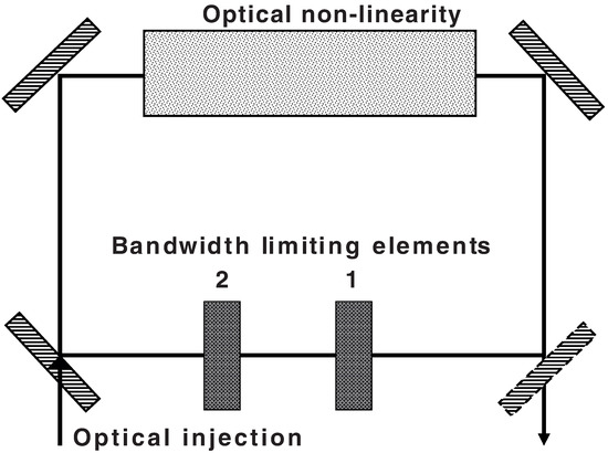
Figure 1. Schematic representation of the considered device.

2.1. Transfer Function of the Filter

The transfer function of the two filters shown in Figure 1 can be written in the standard form [30,31]

$$F\left(\omega \right)=e^{f\left(\omega \right)},$$

(3)

where the complex function $f\left(\omega \right)$ can be expanded in power series near $\omega =0$

$$f\left(\omega \right)=\sum _k{D}_k{\omega }^k,$$

(4)

and $\Im D_k$ represents the dispersion of the kth order. ( For example, for a single Lorentzian absorption line we have $f=\frac{-\sigma L}{\Gamma +i(\omega +\Omega )}$ [31], and second-order dispersion coefficient takes the form $\Im D_2=\Im \frac{d^{2}f}{d{\omega }^2}\approx \frac{2\sigma L}{{\Omega }^3}$ for $0<\Gamma \ll |\Omega |$, and the sign of the coefficient coincides with the sign of $\Omega$.)

From Equations (1) and (2) one obtains that the two filter transfer function is

$$F\left(\omega \right)=\frac{{\gamma }_1{\gamma }_2}{\left[{\gamma }_1+i(\omega -{\omega }_1)\right]\left[{\gamma }_2+i(\omega -{\omega }_2)\right]}.$$

(5)

Since in the frequency domain the transfer functions of two filters are multiplied, see Equation (5), their ordering does not play any role. Therefore, without loss of generality we can assume that ${\gamma }_1\ge {\gamma }_2$ and the reference frequency is chosen in such a way that the maximum of the function $\left|F\right(\omega \left)\right|$ is at $\omega =0$, so that ${\left[\frac{d\left|F\right(\omega \left)\right|}{d\omega }\right]}_{\omega =0}=0$. The latter condition is equivalent to

$${\delta }_F={\gamma }_2^2{\omega }_1+{\omega }_2\left[{\gamma }_1^2+{\omega }_1({\omega }_1+{\omega }_2)\right]=0,$$

(6)

which has two solutions ${\omega }_2={\omega }_{2\pm }=\frac{-{\gamma }_1^2-{\omega }_1^2\pm \sqrt{D_F}}{2{\omega }_1}$, $D_F=-4{\gamma }_2^2{\omega }_1^2+{({\gamma }_1^2+{\omega }_1^2)}^2$. One can see that both ${\omega }_{2\pm }$ can be obtained for any values of ${\omega }_1\ne 0$ and $0<{\gamma }_2<{\gamma }_1$ due to $D_F>0$, and, moreover,

$$|{\omega }_1^2-{\gamma }_1^2|\le \sqrt{D_F}\le {\gamma }_1^2+{\omega }_1^2.$$

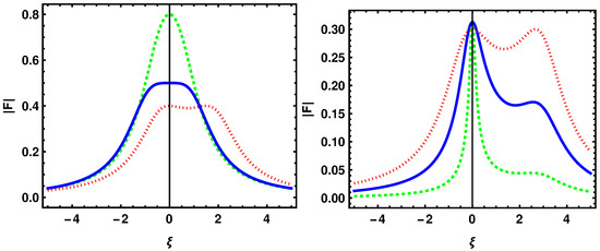
Below we will assume that the condition ${\omega }_2={\omega }_{2+}$ is satisfied that corresponds to a situation when the largest of the two maximums of $\left|F\right(\omega \left)\right|$ is located at zero frequency, see Figure 2. In the left panel of this figure we fix ${\gamma }_1={\gamma }_2=1$ and demonstrate that for ${\omega }_1<1$ we have one global maximum, whereas for ${\omega }_1>1$ we can get two local maxima in our combined filter of the same magnitude. In the second case, or for values of ${\gamma }_2$ close to ${\gamma }_1$, this kind of filter can lead to complex dynamical behaviour in the system, similarly to the case of the Mamyshev oscillator [15,16]. However, in this paper we are focused on the impact of the filter on the frequency of injection, which is assumed to be near or at the global maximum at zero frequency. In the right panel we can observe how the second maximum is suppressed with ${\gamma }_2$ decreasing from 1 to $\frac{1}{8}$. For ${\omega }_2={\omega }_{2+}$ we have

$$\begin{array}{c}{\omega }_2{\omega }_1<0,\left|{\omega }_2\right|\le \left|{\omega }_1\right|,\left|\frac{d{\omega }_2}{d{\omega }_1}\right|<1,\end{array}$$

and one can see that

$$\frac{d|{\omega }_2-{\omega }_1|}{d\left|{\omega }_1\right|}>0,$$

i.e., the difference between the two frequencies grows with $\left|{\omega }_1\right|$, and since for any of ${\omega }_1=\pm {\omega }_1^{*}$ we have ${\omega }_2=\mp {\omega }_2^{*}$, respectively, for any fixed $0<{\gamma }_2<{\gamma }_1$ we can choose $|{\omega }_2-{\omega }_1|$ and find corresponding value of ${\omega }_1$ (negative or positive) and ${\omega }_2={\omega }_{2+}$, which means that we can have any possible combinations of two filters (narrow filter to the left or to the right of the broad filter), disregarding frequency shift of the combined filter. Moreover, these inequalities immediately imply that the largest maximum of $\left|F\right(\omega \left)\right|$ is at $\omega =0$ for ${\omega }_2={\omega }_{2+}$ as claimed earlier, since more narrow Lorentzian filter with the width ${\gamma }_2$ has the central frequency ${\omega }_2$ closer to zero frequency. The other root (6) ${\omega }_2={\omega }_{2-}$ can correspond to a global maximum, a local maximum, or a local minimum, which do not provide any additional useful alternatives, if we are interested to fix the maximum of the combined filter $\left|F\right(\omega \left)\right|$ at zero frequency $\omega =0$.

Figure 2. Absolute value of the transfer function F defined by Equation (5), where ${\omega }_2={\omega }_{2+}$ satisfies (6), ${\gamma }_1=1$ and other parameters are varied: (left) ${\gamma }_2=1$, ${\omega }_1=\frac{1}{2}$ (dashed), ${\omega }_1=1$ (solid), ${\omega }_1=2$ (dotted); (right) ${\omega }_1=3$, ${\gamma }_2=\frac{1}{8}$ (dashed), ${\gamma }_2=\frac{1}{2}$ (solid), ${\gamma }_2=1$ (dotted). The corresponding values of ${\omega }_2$, $\beta$, $\sigma$ are $\{-\frac{1}{2},-1,-\frac{1}{2}\}$, $\{0,0,\frac{3}{4}\}$ and $\{\frac{4}{\sqrt{5}},\sqrt{2},\frac{5}{\sqrt{8}}\}$ (left); $\{-0.0047,-0.07677,-\frac{1}{3}\}$, $\{2.66,1.95,\frac{4}{3}\}$ and $\{8.58,3.84,\frac{5\sqrt{2}}{3}\}$ (right).

Since $f\left(\omega \right)=lnF\left(\omega \right)$, in the power series expansion (4) we obtain the second-order coefficient as

$$D_2=\frac{{\omega }_1^2-{\gamma }_1^2-2i{\gamma }_1{\omega }_1}{2{({\gamma }_1^2+{\omega }_1^2)}^2}+\frac{{\omega }_2^2-{\gamma }_2^2-2i{\gamma }_2{\omega }_2}{2{({\gamma }_2^2+{\omega }_2^2)}^2}.$$

One can check that $D_2$ can be represented in the following way

$$\begin{array}{c}{D}_2=\rho \left(-\frac{{\sigma }^2-2}{2}+i\beta \right)+\frac{{\delta }_F\left[{\delta }_F-2i\left({\gamma }_1^2{\gamma }_2+{\gamma }_1{\gamma }_2^2+{\gamma }_2{\omega }_1^2+{\gamma }_1{\omega }_2^2\right)\right]}{2\left({\gamma }_1^2+{\omega }_1^2\right)\left({\gamma }_2^2+{\omega }_2^2\right)({\gamma }_1{\gamma }_2-{\omega }_1{\omega }_2)},\end{array}$$

(7)

with

$$\begin{array}{c}\rho =\frac{{\gamma }_1{\gamma }_2-{\omega }_1{\omega }_2}{\left({\gamma }_1^2+{\omega }_1^2\right)\left({\gamma }_2^2+{\omega }_2^2\right)},\end{array}$$

(8)

$$\begin{array}{c}\sigma =\frac{\sqrt{\rho }\left({\gamma }_1^2{\gamma }_2+{\gamma }_1{\gamma }_2^2+{\gamma }_2{\omega }_1^2+{\gamma }_1{\omega }_2^2\right)}{{\gamma }_1{\gamma }_2-{\omega }_1{\omega }_2},\end{array}$$

(9)

$$\begin{array}{c}\beta =\frac{{\gamma }_1{\omega }_2+{\gamma }_2{\omega }_1}{{\gamma }_1{\gamma }_2-{\omega }_1{\omega }_2}.\end{array}$$

(10)

It follows from the conditions (6), where ${\omega }_2={\omega }_{2+}$, and the relation ${\gamma }_1\ge {\gamma }_2$ that the second term in the right hand side (RHS) of (7) vanishes, $\rho >0$, and $\mathrm{sign}\beta =\mathrm{sign}{\omega }_1$. Hence, the parameters $\beta$ and $\frac{{\sigma }^2-2}{2}$ represent the normalized second-order dispersion and the diffusion near zero frequency, respectively, whereas the parameter $\sqrt{\rho }$ can be considered as a scaling coefficient.

One can see that under these conditions

$$\frac{d\left|\beta \right|}{d\left|{\omega }_1\right|}>\frac{\sqrt{D}(\sqrt{D}+{\omega }_1^2-{\gamma }_1^2)}{4{\gamma }_1{\omega }_1^2({\gamma }_1^2+{\omega }_1^2)}>0,$$

and since $|{\omega }_2-{\omega }_1|$ grows with $\left|{\omega }_1\right|$, second-order dispersion grows with the difference between the frequencies. Moreover, using (6) to express ${\omega }_2^2$ one obtains

$$\begin{array}{c}\sigma =\frac{({\gamma }_2{\omega }_1-{\gamma }_1{\omega }_2)\mathrm{Sign} {\omega }_1}{\sqrt{{\omega }_1{\omega }_2({\omega }_1{\omega }_2-{\gamma }_1{\gamma }_2)}},\\ \frac{d\sigma }{d{\gamma }_2}=\frac{\left|{\omega }_1\right|({\gamma }_1{\gamma }_2{\omega }_1+({\gamma }_1^2-2{\omega }_1^2){\omega }_2)({\gamma }_2\frac{d{\omega }_2}{d{\gamma }_2}-{\omega }_2)}{2{\left({\omega }_1{\omega }_2({\omega }_1{\omega }_2-{\gamma }_1{\gamma }_2)\right)}^{3/2}},\\ {\gamma }_2\frac{d{\omega }_2}{d{\gamma }_2}-{\omega }_2={\omega }_2\frac{{\gamma }_1^2+{\omega }_1^2}{2\sqrt{D}},\\ {\omega }_1({\gamma }_1{\gamma }_2{\omega }_1+({\gamma }_1^2-2{\omega }_1^2){\omega }_2)<-\frac{{\gamma }_1^2({\gamma }_1^2+{\omega }_1^2)}{2},\end{array}$$

hence due to ${\omega }_1{\omega }_2<0$ we see that $\frac{d\sigma }{d{\gamma }_2}<0$, and $\sigma$ decreases with ${\gamma }_2$ increasing from 0 to ${\gamma }_1$. Therefore, the lower bound on $\sigma$ can be estimated assuming ${\gamma }_2={\gamma }_1$, where ${\omega }_2=\frac{-{\gamma }_1^2-{\omega }_1^2+|{\omega }_1^2-{\gamma }_1^2|}{2{\omega }_1}$ and

$$\sigma \ge {\sigma }_{{\gamma }_2={\gamma }_1}=\left\{\begin{array}{cc}\begin{array}{c}\sqrt{2}\sqrt{1+{\beta }^2},\left|{\omega }_1\right|\ge {\gamma }_1,\hfill \\ 2\frac{{\gamma }_1\sqrt{1+{\beta }^2}}{\sqrt{{\gamma }_1^2+{\omega }_1^2}},\left|{\omega }_1\right|<{\gamma }_1.\hfill \end{array}& \ge \sqrt{2}\sqrt{1+{\beta }^2}.\end{array}\right.$$

(11)

2.2. Normalized DDE Model

By substituting Equation (2) into Equation (1), using Equation (6), and rescaling time as $t\to t/\sqrt{\rho }$, we obtain the following normalized dimensionless second-order DDE

$$\begin{array}{c}{A}^{″}\left(t\right)(1+i\beta )+\sigma A^{\prime }\left(t\right)+A\left(t\right)=\sqrt{\kappa }{e}^{i\alpha {\left|A(t-T)\right|}^2+i\phi }A(t-T)+\eta e^{i{\omega }_{0}t},\\ \sigma >\sqrt{2}\sqrt{1+{\beta }^2},\end{array}$$

(12)

where losses and forcing take the form $\sqrt{\kappa }=r\sqrt{{\kappa }_l}\le 1$, $\eta =r{\eta }_0$ with $r=\frac{{\gamma }_1{\gamma }_2}{\sqrt{({\gamma }_1^2+{\omega }_1^2)({\gamma }_2^2+{\omega }_2^2)}}\le 1$, and the phase shift is $\phi =\varphi +arg\frac{1}{{\gamma }_2{\gamma }_2-{\omega }_1{\omega }_2-i({\gamma }_1{\omega }_2+{\omega }_2{\gamma }_1)}$. Here, similarly to the previous section one can see that $\frac{dr}{d\left|{\omega }_1\right|}<0$ for ${\gamma }_1>{\gamma }_2$ and ${\omega }_2={\omega }_{2+}$, hence for fixed ${\kappa }_l$ the parameter $\kappa$ decreases with increasing detuning between the two frequencies $|{\omega }_2-{\omega }_1|$. With the condition (11) on dimensionless parameters $\sigma$ and $\beta$ the equation is equivalent to the system with two filters (1) and (2) for any $\kappa <1$ with global maximum of the combined filter transfer function $F\left(\omega \right)$ (5) located at zero frequency $\omega =0$, $\left|F\right(\omega \left)\right|\le \left|F\right(0\left)\right|\le 1$. We note that for $\sqrt{2}\le \sigma \le \sqrt{2(1+{\beta }^2)}$ the global maximum of $F\left(\omega \right)$ is at another frequency and additional constraints on parameter $\kappa$ are necessary, whereas for $\sigma <\sqrt{2}$ the diffusion coefficient in (7) becomes negative, equivalence with (1) and (2) is lost and zero solution $A=0$ for $\eta =0$ is unstable.

For $\beta =0$ relation (7) gives zero dispersion coefficient and diffusion coefficient equal to $({\sigma }^2-2)/2$, which agrees with previous analysis of a similar DDE [39] in case of $\sigma >\sqrt{2}$.

We note that the direct application of truncated expansion (4) in the RHS of DDE models similar to (1) and (12) would lead to the appearance of the second derivative of the delayed variable $A^{″}(t-T)$ in and spurious instability [31]. In contrast, non-delayed second order derivative $A^{″}\left(t\right)$ in (12) appears without any expansions, and the term $i\beta A^{″}\left(t\right)$ is responsible for the second-order chromatic dispersion similarly to the CGL equations. On the other hand, unlike the cubic CGL model, where the real coefficient by the second derivative is responsible for the diffusion (or parabolic spectral filtering), the filtering in (12) is performed by two Lorentzian filters, which are introduced by the presence of of both the first and the second order derivatives. Therefore, the generality of this kind of dispersion operator is still not directly comparable to the operators in CGL-type equations or systems with distributed delay [31]. However, in contrast to the approximate DDEs [32], the physical meaning of this filter is clear for any feasible parameters. For simplicity below we consider the case of non-detuned injection, ${\omega }_0=0$.

2.3. Limit of Lugiato-Lefever Equation

Assuming large delay limit $T=r/\epsilon$, where $\epsilon \ll 1$ and $r=1+a_1\epsilon +a_2{\epsilon }^2+\dots$, taking ${\omega }_0=0$, and rescaling the time variable $t\to t/\epsilon$ we can rewrite (12) in the form

$$\begin{array}{c}{\epsilon }^2{A}^{″}\left(t\right)(1+i\beta )+\epsilon \sigma A^{\prime }\left(t\right)+A\left(t\right)=\sqrt{\kappa }{e}^{i\alpha {\left|A(t-r)\right|}^2+i\phi }A(t-r)+\eta ,\end{array}$$

(13)

Let the injection rate, the linear cavity losses and the phase shift be small,

$$\eta ={\epsilon }^{3}S,\kappa =1-2{\epsilon }^{2}k,\phi ={\epsilon }^2\theta .$$

(14)

Then looking the solution in the form $A\left(t\right)=\epsilon u(t,\tau )+{\epsilon }^{2}v(t,\tau )+\dots$ with $\tau ={\epsilon }^{2}t$, applying multiscale analysis [40,41], collecting the first order in $\epsilon$, and using solvability condition of the resulting equation we get the periodic boundary condition:

$$u(t,\tau )=u(t-1,\tau ).$$

(15)

Next, in the second order in $\epsilon$ we obtain

$$\begin{array}{c}v(t,\tau )-v(t-1,\tau )=a_1{u}_t(t-1,\tau )-\sigma u_t(t,\tau ),\end{array}$$

which implies the periodicity of v, $v(t-1,\tau )=v(t,\tau )$ and the relation $a_1=\sigma$ with the periodicity condition (15). Finally collecting the third order terms in $\epsilon$, using the relation $a_2={\sigma }^2$, and applying solvability condition [40,41] we get the generalized Lugiato-Lefever equation (LLE)

$$u_{\tau }=S-ku+i\theta u+i\alpha u{\left|u\right|}^2+\left(\frac{{\sigma }^2-2}{2}-i\beta \right)u_{tt}$$

(16)

with the diffusion coefficient $({\sigma }^2-2)/2$ and the boundary condition (15). It is well known that for $\beta <0$ in Equation (16) corresponds to anomalous dispersion regime, and for $\theta <0$ this equation can demonstrate the formation of bright dissipative solitons [35]. Dimensionless dispersion and diffusion coefficients in Equation (16) coincide with those defined by Equation (7).

3. Continuous Wave (CW) State

The CW state of the Equation (12) with ${\omega }_0=0$ takes the form $A=A_0{e}^{i\psi }$, where the real quantities $A_0$ and $\psi$ satisfy the system of the transcendental equations

$$\begin{array}{c}{A}_0\left[1-\sqrt{\kappa }cos\left(\alpha A_0^2+\phi \right)\right]=\eta cos\psi ,\end{array}$$

(17)

$$\begin{array}{c}{A}_0\sqrt{\kappa }sin\left(\alpha A_0^2+\phi \right)=\eta sin\psi ,\end{array}$$

(18)

which leads to a single transcendental equation for $A_0^2$

$$\begin{array}{c}{A}_0^2\left[\kappa +1-2\sqrt{\kappa }cos\left(\alpha A_0^2+\phi \right)\right]={\eta }^2.\end{array}$$

(19)

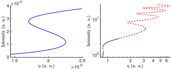
Assuming $\epsilon \ll 1$, $A_0=\epsilon u_0$, $\phi ={\epsilon }^2\theta$, $0<1-\kappa$∼$2{\epsilon }^{2}k$, and $\eta ={\epsilon }^{3}S$, this equation can be approximated by a cubic equation for $u_0^2$

$$S^2\approx u_0^2\left[k^2+{(\theta +\alpha u_0^2)}^2\right],$$

(20)

which coincides with the equation for the uniform stationary solutions of the LLE (16). Therefore, in this limit Equation (12) can have up to three coexisting CW states similarly to LLE (see Figure 3, left), however out of this limit for strong injection there can be more coexisting CW states, see right panel of Figure 3. Here, the upper CW state looses stability via a modulational instability, and unstable CW states are shown by dotted red line.

Figure 3. Intensity ${\left|A_0\right|}^2$ of CW states (17) and (18) obtained by varying parameter $\eta$ (left). Here, ${\omega }_0=0$, $\kappa =1-{10}^{-4}$, $\sigma =\sqrt{2.5}$, $\alpha =1$, $\phi =-3\times {10}^{-4}$, which in the LLE limit (13) corresponds to $\epsilon =0.01$. In the right panel we choose $\kappa =exp(-2)$, $\phi =-2$, which corresponds to $\epsilon =1$, where solid lines correspond to stable CWs and dashed - to unstable.

Stability of CW Solution and MI

Here, we demonstrate how MI of an initially stable CW state can appear in the anomalous dispersion regime in the limit of large delay $T\gg 1$. For that, we linearize the Equation (12) near the CW state $A\left(t\right)=(A_0+\delta A{e}^{\lambda t})e^{i\psi }$ and calculate the determinant of the Jacobian of the linearised system to obtain the following characteristic equation for the eigenvalues $\lambda$ describing the stability of the CW solution:

$$\begin{array}{c}\hfill \kappa Y^2+\lambda \{\lambda \left[\left({\beta }^2+1\right){\lambda }^2+2\lambda \sigma +{\sigma }^2+2\right]+2\sigma \}+1+\\ \hfill 2\sqrt{\kappa }Y\{sin\left(\alpha A_0^2+\phi \right)\left[\alpha A_0^2\left({\lambda }^2+\lambda \sigma +1\right)-\beta {\lambda }^2\right]-\\ \hfill cos\left(\alpha A_0^2+\phi \right)\left[{\lambda }^2\left(\alpha A_0^2\beta +1\right)+\lambda \sigma +1\right]\}=0.\end{array}$$

(21)

where $Y\left(\lambda \right)=exp(-\lambda T)$. In the limit of large delay time $T\to \infty$ the eigenvalues belonging to the pseudo-continuous spectrum can be represented in the form $\lambda =i\mu +\frac{\Lambda }{T}+\mathcal{O}(1/T^2)$ with real $\mu$ [42]. Thus, in this limit the characteristic equation is a quadratic equation for Y with the coefficients depending only on the imaginary part $\mu$ of the eigenvalue, and we can obtain from (21) two branches of pseudo-continuous spectrum given by

$${\Lambda }_{\pm }\left(\mu \right)=-\Re ln{Y}_{\pm }\left(i\mu \right).$$

(22)

For a stable CW solution we have ${\Lambda }_{\pm }\left(\mu \right)\le 0$ and, in particular, ${\Lambda }_{\pm }\left(0\right)=-\Re ln{Y}_{\pm }\left(0\right)\le 0$, where

$$\begin{array}{c}{Y}_{\pm }\left(0\right)=\frac{1}{\sqrt{\kappa }}\left[cos\left(\alpha A_0^2+\phi \right)-\alpha A_0^{2}sin\left(\alpha A_0^2+\phi \right)\pm \sqrt{D}\right],\end{array}$$

(23)

$$\begin{array}{c}D={\left[cos\left(\alpha A_0^2+\phi \right)-\alpha A_0^{2}sin\left(\alpha A_0^2+\phi \right)\right]}^2-1.\end{array}$$

(24)

Moreover, the second derivative of ${\Lambda }_{\pm }\left(\mu \right)$ at $\mu =0$ takes the form

$$\begin{array}{c}{\Lambda }_{\pm }^{″}\left(0\right)=2-{\sigma }^2\pm 2\beta \Re \mathcal{B}(\alpha ,\phi ,\eta ,\kappa ),\end{array}$$

(25)

$$\begin{array}{c}\mathcal{B}=\frac{\alpha A_0^{2}cos\left(\alpha A_0^2+\phi \right)+sin\left(\alpha A_0^2+\phi \right)}{\sqrt{D}}.\end{array}$$

(26)

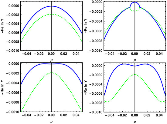
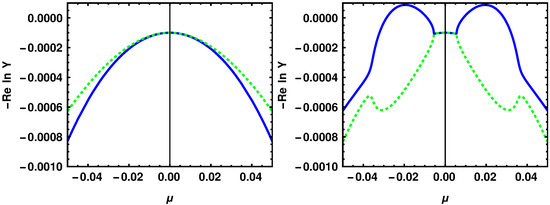
One can see from (25) that for small $\beta \approx 0$ and $\sigma >\sqrt{2}$ we have ${\Lambda }_{\pm }^{″}\left(0\right)<0$ for the CW solutions on the upper branch of S-shaped bifurcation curve depicted in Figure 3 (see top-left panel of Figure 4). It is known that strong anomalous dispersion can lead to the change of the curvature of one of the two branches ${\Lambda }_{\pm }\left(\mu \right)$ of the pseudo-continuous spectrum at $\mu =0$ (see Figure 4, bottom-left) [31]. Moreover, further increase of anomalous dispersion can lead to a MI of a CW state (see Figure 4, bottom-right) [32]. On the other hand, in the case of strong normal dispersion regime the sign change of the curvature of the curve with smaller ${\Lambda }_{\pm }\left(0\right)$ does not lead to a MI, as it is seen from the top-right panel of Figure 4.

Figure 4. Curves of pseudocontinuous spectrum in the limit of large delay (21) of (12) of the CW with the largest intensity ($\left|A_0\right|\approx 0.0169$ out of another two $\left|A_0\right|\approx 0.0167$ and $\left|A_0\right|\approx 0.006$) near the LLE limit, $\eta \approx 1.707\times {10}^{-6}$, and varying $\beta =0$ (top-left), $\beta =1/4$ (top-right), $\beta =-1/8$ (bottom-left), $\beta =-1/4$ (bottom-right). Other parameters are as in Figure 3.

The stability condition of the CW state can be written in the form $\left|Y_{\pm }\left(i\mu \right)\right|>1$ for all the wavenumbers $\mu$. In particular, at zero wavenumber $\mu =0$ we get

$$\left|Y_{\pm }\left(0\right)\right|>1.$$

(27)

A CW solution satisfying this condition is stable with respect to perturbations at zero wavenumber, but may be unstable with respect to MI at nonzero wavenumbers. A possible (but not unique) way how such a MI can develop is related to the change of the sign from negative to positive of one of the two quantities ${\Lambda }_{\pm }^{″}\left(0\right)$ corresponding to the greater of the two values ${\Lambda }_{\pm }^{″}\left(0\right)$. Note, that both the quantities ${\Lambda }_{\pm }^{″}\left(0\right)$ are always negative at $\beta =0$ due to the inequality (11). It follows from Equation (26) that such a sign change can take place only in the case when

$$D>0$$

(28)

and, hence, $Y_{\pm }\left(0\right)$ must be real. Otherwise, $\mathcal{B}$ is purely imaginary and the last term in the RHS of Equation (25) vanishes. It is shown in Appendix A that in the LLE limit (14) we have ${\Lambda }_{+}\left(0\right)<{\Lambda }_{-}\left(0\right)$ and for the CW state with the highest intensity we can have ${\Lambda }_{-}^{″}\left(0\right)>0$ only in the anomalous dispersion regime $\beta <0$. Out of LLE limit we can have positive ${\Lambda }_{\pm }^{″}\left(0\right)$ in case of $\beta >0$ as well (see Appendix B for numerical treatment).

Note, that the development of MI on the stable upper part of the CW branch can be correlated with the appearance of stable localized structures. In the next section we study numerically how the dispersion coefficient $\beta$ affects the existence range of these structures. Remarkably, there are also scenarios out of the LLE limit where localized structures can be observed for zero and small positive $\beta$.

We note that the condition ${\Lambda }^{″}\left(0\right)>0$ precedes the appearance of MI of the CW for stronger dispersion if $Y_{\pm }\left(0\right)$ is real-valued. If it is complex-valued, MI is still possible for sufficiently strong dispersion (see Figure 5). In the LLE limit, one can derive an approximate condition for MI development (see Appendix A), and demonstrate that for typical parameters in this limit strong anomalous dispersion can lead to the instability.

Figure 5. Curves of pseudocontinuous spectrum in the limit of large delay (21) of (12) of the CW with the largest intensity ($\left|A_0\right|\approx 0.0178$ out of another two $\left|A_0\right|\approx 0.0156$ and $\left|A_0\right|\approx 0.0065$) near the LLE limit with $\beta =1/2$ (left) and $\beta =1/2$ (right), and $\eta \approx 1.797\times {10}^{-6}$. Other parameters are as in Figure 3.

4. Numerical Results

In this section, we perform numerical bifurcation analysis of Equation (12) using DDE-BIFTOOL [43]. Let us start with the parameter set close to the LLE limit. We take $\sigma =\sqrt{2.5}$, $\beta =-0.5$, which corresponds to two filters (5) with ${\gamma }_1={\gamma }_2$, ${\omega }_1=-\frac{1+\sqrt{5}}{2}{\gamma }_1\approx -1.62{\gamma }_1$, ${\omega }_2=\frac{\sqrt{5}-1}{2}{\gamma }_2\approx 0.62{\gamma }_2$. Let $\alpha =1$, ${\omega }_0=0$ and $\phi ={\phi }_{\epsilon }$, $\kappa ={\kappa }_{\epsilon }$, where

$${\kappa }_{\epsilon }=exp(-2{\epsilon }^2),{\phi }_{\epsilon }=-2{\epsilon }^2$$

are chosen according to analysis of DDE (13) in the limit $\epsilon \to 0$. These values directly correspond to the parameters of LLE (16) where localized structures are known to exist ($\theta =\phi /{\epsilon }^2<-\sqrt{3}$). We also pick a reference injection strength

$${\eta }_{\epsilon }={\epsilon }^3\sqrt{\frac{8}{{\sqrt{3}}^3}+\frac{4}{3}\left(-\frac{{\phi }_{\epsilon }}{{\epsilon }^2}-\sqrt{3}\right)},$$

(29)

where three CW states are guaranteed to coexist for $\epsilon \ll 1$, and vary $\eta$ near ${\eta }_{\epsilon }$. The main numerical difficulty in this limit is that the delay time T and the width of the localized structures are proportional to the large quantity ${\epsilon }^{-1}$. Figure 6 was obtained with $\epsilon =0.05$, which was the smallest value of $\epsilon$ used in our simulations and corresponded to $\kappa \approx 0.995$. Similarly to the LLE [44,45] the bifurcation diagram in the left panel of this figure shows a typical S-shaped CW branch with stable lower part and modulationally unstable upper part. The branch of unstable periodic solutions bifurcates from the unstable middle part of the CW branch and it becomes stable after a fold bifurcation at $\eta \approx 0.00022$. The stable periodic solution has only a slight asymmetry in its time profile and resembles the temporal dissipative solitons of the LLE, see right panel of Figure 6.

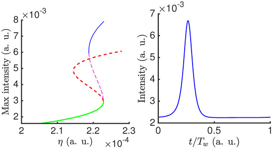
Figure 6. Left panel: One-parameter bifurcation diagram of Equation (12) with $\phi ={\phi }_{\epsilon }$, $\kappa ={\kappa }_{\epsilon }$, and $\epsilon =0.05$. CW (periodic) solutions are shown by thick (thin) lines. Solid lines represent stable states and dashed lines represent unstable states. The parameter $\eta$ is changed near ${\eta }_{\epsilon }$ defined by Equation (29). Right panel: Stable localized periodic solution for $\eta \approx 0.000223$, where $T_w$∼$1/\epsilon$ is the period of the solution controlled by the choice of delay time T. Other parameters are $\alpha =1$, $\sigma =\sqrt{2.5}$, $\beta =-0.5$.

Thus, close to the limit $\epsilon \to 0$ the normalized second-order DDE (12) demonstrates the bifurcation structure similar to that of the LLE. Note, however, that the magnitude of the parameters $\sigma$, $\beta$ and $1-\kappa$ in the normalized Equation (12) depends on the frequency detuning of the linear filters with respect to each other in the original equivalent system (1) and (2), and stronger detuning results for fixed $\sigma$ in larger $\left|\beta \right|$ as discussed in Section 2.1, and higher losses $1-\kappa$ at the same time as discussed in Section 2.2. Therefore, it is necessary to investigate how larger values of $\epsilon$ corresponding to smaller values of the attenuation factor $\kappa$ (larger losses) affect the properties of the localized solutions. For example, for the considered parameters $\sigma =\sqrt{2.5}$ and $\beta =-0.5$ from Equations (1) and (2) and the condition ${\kappa }_l\le 1$ one obtains $\kappa \le 0.4$ in (12), which is satisfied for $\epsilon \ge 0.7$.

For larger $\epsilon =0.2$, which corresponds to $\kappa \approx 0.92$, the stable part of the periodic solution branch is split into two parts separated by two fold bifurcation points, see left panel of Figure 7. Both these parts correspond to very asymmetric localized pulses, but the second part contains wider pulses then the first one, see right panel of Figure 7. Figure 8 and Figure 9 show the branches of CW and periodic solutions with scaled intensity (In these figures $\eta$ is shifted, more precisely, $\stackrel{\sim }{\eta }=\eta -{\eta }_{\epsilon }-{\eta }_{1,j}+{10}^{-5}j$ for the left panel of Figure 8, $\stackrel{\sim }{\eta }=\eta -{\eta }_{\epsilon }-{\eta }_{2,j}+5j{\eta }_{2,1}$ for the right panel, $\stackrel{\sim }{\eta }=\eta -{\eta }_{\epsilon }-{\eta }_{1,j}+{10}^{-2}(j-4)$ for the left panel of Figure 9, $\stackrel{\sim }{\eta }=\eta -{\eta }_{\epsilon }-{\eta }_{2,j}+2\times {10}^{-3}(j-4)$ for the right panel, and $\epsilon ={ϵ}_j$, $\overrightarrow{ϵ}=\{0.05,0.1,0.2,0.3,0.4,0.5,0.6,0.7,0.8,0.9,1.0\}$, ${\overrightarrow{\eta }}_1=\{-1.2\times {10}^{-5},-1.634\times {10}^{-4},$ $-7.69\times {10}^{-4},-0.0039,-0.0136,-0.0245,-0.059,-0.11,-0.195,-0.347,-0.5474\}$, ${\overrightarrow{\eta }}_2=\{1.413\times {10}^{-6},4.3\times {10}^{-6},-1.2\times {10}^{-4},-0.0015,-0.006,-0.019,-0.047,-0.099$, $-0.185-0.333,-0.5294\}$) obtained by increasing gradually $\epsilon$ up to 1, which corresponds to $\kappa \approx 0.135$. The width of the S-shaped area of the CW branches as well as the width of the branch of the localized solutions increases with $\epsilon$ up to $\epsilon =0.8$ and then decreases. For $\epsilon \ge 0.4$ the upper branch of CW states stabilizes for the chosen parameter values (Figure 9, left). Asymmetric localized structures corresponding to the stable parts of the periodic solution branches with $\epsilon \ge 0.2$ in Figure 10 look similar to the those shown in the right panel of Figure 7 obtained for $\epsilon =0.2$.

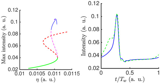
Figure 7. Left panel: One-parameter bifurcation diagram of Equation (12) with $\phi ={\phi }_{\epsilon }$, $\kappa ={\kappa }_{\epsilon }$, and $\epsilon =0.2$. CW (periodic) solutions are shown by thick (thin) lines. Solid lines represent stable states and dashed lines represent unstable states. The parameter $\eta$ is changed near ${\eta }_{\epsilon }$ defined by Equation (29). Right panel: Stable localized periodic solutions for the same $\eta$ from the first (main) stable part of the periodic solution branch (solid) and the secondary stable part (dashed). Other parameters are as in Figure 6.

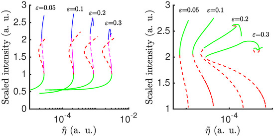
Figure 8. Bifurcation diagrams of Equation (12) obtained for different values of $\epsilon$. Left panel: CW states cut around S-shaped bifurcation curve (thick lines) and periodic solutions (thin lines). Solid lines represent stable states and dashed lines represent unstable states, $\stackrel{\sim }{\eta }=\eta -{\eta }_{\epsilon }+\delta \eta \left(\epsilon \right)$ is a shifted value of $\eta$. Right panel: Branches of periodic solutions from the left panel, magnified. The intensity is scaled by ${\epsilon }^2$ and other parameters are as in Figure 6.

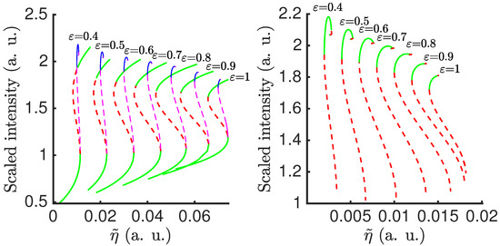
Figure 9. CW states cut around S-shaped bifurcation curve (thick lines) and periodic solutions (thin lines) of (12), where solid lines represent stable states and dashed lines represent unstable states. Right panel: Branches of periodic solutions from the left panel, magnified. The intensity is scaled by ${\epsilon }^2$, the curves from left to right correspond to $j=5,6,7,8,9,10,11$, and other parameters are as in Figure 8.

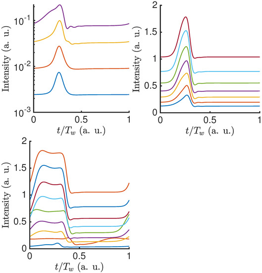
Figure 10. Top panels: Localized periodic solutions of Equation (12) from the middle points of the stable parts of the branches depicted on Figure 8 and Figure 9 for $\epsilon$ increasing from 0.05 (bottom curve of the left upper panel) to 1 (top curve of the bottom panel). Bottom panel: Wider localized solutions from the secondary parts of the periodic solution branches for $\epsilon$ increasing from 0.2 (bottom curve) to 1 (top curve). Time is scaled by the solution period $T_w$∼${\epsilon }^{-1}$, which is controlled by the delay time T. Other parameters are as in Figure 8.

Finally, let us study how the variation of the effective dispersion coefficient $\beta$ influences the existence range of the temporal localized structures. One can see in the top left panel of Figure 11 that near the LLE limit ($\epsilon =0.05$) the localized solutions can be observed only for negative $\beta <-0.05$ corresponding to the anomalous dispersion regime. It is seen that when $\beta$ increases the interval of the injection rates between two fold bifurcations, where stable localized solutions exist, shrinks so that for $\beta \ge -0.06$ one can hardly see any stable localized structure in the region of S-shaped CW curve. However, by increasing $\epsilon$ out of the LLE limit first to $\epsilon =0.3$ (top right panel of Figure 11) and then to $\epsilon =0.5$ (bottom left panel), one can see that around $\epsilon \approx 0.5$ localized structures can be observed for $\beta =0$ as well. Furthermore, for $0.5\le \epsilon \le 1$ (bottom right panel) stable bright temporal dissipative solitons can be observed even with small positive $\beta$, $0\le \beta <0.1$. Therefore, we conclude that out of the LLE limit temporal localized structures in the DDE model (12) could be observed not only in anomalous dispersion regime but also for positive $\beta$, although in a smaller range of the injection rates $\eta$. We have considered here only one possible way to exit the LLE limit in a continuous manner, however our preliminary numerical simulations suggest that there are many possible combinations of values of $\kappa$, $\eta$, $\phi$, and $\beta$ away from the LLE limit, where stable or unstable temporally localized structures can be observed. We leave this question to further studies, and, in particular, for experimentally justified parameters.

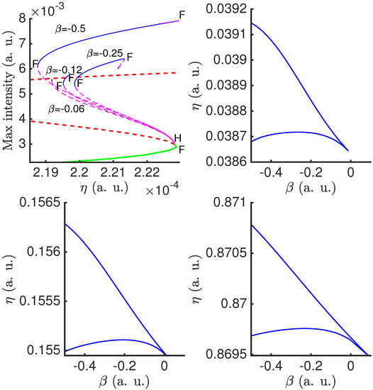
Figure 11. Top left: Bifurcation diagram of Equation (12) for $\epsilon =0.05$ and various values of $\beta$. Thick lines indicate CW solutions cut around S-shaped bifurcation curve, while thin lines correspond to periodic solutions. Solid (dashed) lines represent stable (unstable) solutions. Fold bifurcations are marked by F and Hopf bifurcations are marked by H. Other panels show fold bifurcations of the localized periodic solutions of (12) on the plane of two parameters, $\beta$ and $\eta$. They correspond to $\epsilon =0.3$ (top right), $\epsilon =0.5$ (bottom left), and $\epsilon =1.0$ (bottom right). Other parameters are as in Figure 8.

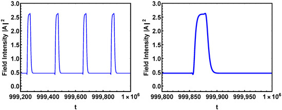
In this section we have demonstrated the existence of bright localized structures of the second oder DDE model (12). It follows from this result that such kind of structures should also exist in the original set of two DDEs (1) and (2). We can use this theory then to find parameters for (1) and (2) where localized structures exist (see Figure 12).

Figure 12. Periodic pulse train solution $A\left(t\right)$ of (1) and (2) (left) and single pulse (right), where the parameters are ${\gamma }_1=1$, ${\omega }_1\approx 1.29$, ${\gamma }_2\approx 0.26$, ${\omega }_2\approx -0.034$, ${\kappa }_l\approx 0.68$, $\varphi \approx -4.17$, ${\eta }_0\approx 1.65$, $\alpha =1.5$, $T=200$. In the normalized Equation (12) these values correspond to $\sigma =3.23$, $\beta =1$, $\kappa =0.25$, $\phi \approx -3.383$, $\eta =1$.

5. Conclusions

We have considered a DDE model of an optically injected ring Kerr cavity with two spectral filters having different widths and central frequencies. We have derived a normalized complex-valued second order DDE (12), which is similar to real-valued DDE reported in [39]. This equation can be considered as a generalization of the Ikeda map, which explicitly contains second-order dispersion coefficient at zero frequency as a parameter. We have derived an admissibility relation for these parameters, analyzed stability of the CW solutions of this model in the limit of large delay, and demonstrated the effect of strong dispersion on the development of modulational instability. We have shown that in the limit of small losses and weak injection the DDE model can be reduced to a generalized version of the well known LLE, which is known to have dissipative soliton solutions. We have performed numerical bifurcation analysis of CW solutions and temporal localized structures using DDE-BIFTOOL package [43] and demonstrated qualitative similarity of the solutions of the DDE model with those of the LLE in the regime of anomalous dispersion ($\beta <0$) in the corresponding limit. Moreover, out of LLE limit one can observe numerically stable asymmetric bright localized structures not only in the anomalous dispersion regime, but also at zero and small positive values of $\beta$, albeit in a shrinkingly smaller interval of existence. This is in agreement with the results of Ref. [46] obtained using an extended LLE with the third order dispersion term included. Experimental observations of asymmetric temporal Kerr cavity solitons near zero dispersion point, where higher order dispersion comes into play, were reported in [47].

To summarize, we have proposed theoretically a Kerr cavity scheme, where the dispersion introduced by two spectral filters with different central frequencies can lead to the development of modulational instability and appearance of stable temporal cavity solitons even when the material dispersion is negligible. This scheme is different from the traditional Kerr cavity setups for frequency comb generation, where chromatic dispersion of the intracavity material plays a crucial role in soliton formation. The modeling approach we have developed is also suitable for the analysis of more complex systems with two spectral filters, such as Mamyshev oscillators. Investigation of short pulse generation in Mamyshev oscillators using the theoretical basis developed here might be a subject for future research.

References

- Fortier, T.; Baumann, E. 20 years of developments in optical frequency comb technology and applications. Commun. Phys. 2019, 2, 153. [Google Scholar] [CrossRef]
- Kippenberg, T.J.; Gaeta, A.L.; Lipson, M.; Gorodetsky, M.L. Dissipative Kerr solitons in optical microresonators. Science 2018, 361, eaan8083. [Google Scholar] [CrossRef]
- Bao, H.; Cooper, A.; Rowley, M.; Di Lauro, L.; Totero Gongora, J.S.; Chu, S.T.; Little, B.E.; Oppo, G.L.; Morandotti, R.; Moss, D.J.; et al. Laser cavity-soliton microcombs. Nat. Photonics 2019, 13, 384–389. [Google Scholar] [CrossRef]
- Wang, W.; Wang, L.; Zhang, W. Advances in soliton microcomb generation. Adv. Photonics 2020, 2, 034001. [Google Scholar] [CrossRef]
- Weiner, A.M. Cavity solitons come of age. Nat. Photonics 2017, 11, 533–535. [Google Scholar] [CrossRef]
- Herr, T.; Brasch, V.; Jost, J.D.; Wang, C.Y.; Kondratiev, N.M.; Gorodetsky, M.L.; Kippenberg, T.J. Temporal solitons in optical microresonators. Nat. Photonics 2014, 8, 145–152. [Google Scholar] [CrossRef]
- Boutabba, N.; Eleuch, H. Slowing light control for a soliton-pair. Appl. Math. Inf. Sci. 2013, 7, 1505. [Google Scholar] [CrossRef]
- Englebert, N.; De Lucia, F.; Parra-Rivas, P.; Arabí, C.M.; Sazio, P.J.; Gorza, S.P.; Leo, F. Parametrically driven Kerr cavity solitons. Nat. Photonics 2021, 15, 857–861. [Google Scholar] [CrossRef]
- Leo, F.; Coen, S.; Kockaert, P.; Gorza, S.P.; Emplit, P.; Haelterman, M. Temporal cavity solitons in one-dimensional Kerr media as bits in an all-optical buffer. Nat. Photonics 2010, 4, 471–476. [Google Scholar] [CrossRef]
- Williams, K.; Thompson, M.; White, I. Long-wavelength monolithic mode-locked diode lasers. New J. Phys. 2004, 6, 179. [Google Scholar] [CrossRef]
- Turaev, D.; Vladimirov, A.G.; Zelik, S. Long-Range Interaction and Synchronization of Oscillating Dissipative Solitons. Phys. Rev. Lett. 2012, 108, 263906. [Google Scholar] [CrossRef] [PubMed]
- Vladimirov, A.G.; Gurevich, S.V.; Tlidi, M. Effect of Cherenkov radiation on localized-state interaction. Phys. Rev. A 2018, 97, 013816. [Google Scholar] [CrossRef]
- Vladimirov, A.G.; Tlidi, M.; Taki, M. Dissipative soliton interaction in Kerr resonators with high-order dispersion. Phys. Rev. A 2021, 103, 063505. [Google Scholar] [CrossRef]
- Dong, X.; Spiess, C.; Bucklew, V.G.; Renninger, W.H. Chirped-pulsed Kerr solitons in the Lugiato-Lefever equation with spectral filtering. Phys. Rev. Res. 2021, 3, 033252. [Google Scholar] [CrossRef]
- Mamyshev, P. All-optical data regeneration based on self-phase modulation effect. In Proceedings of the 24th European Conference on Optical Communication, ECOC’98 (IEEE Cat. No. 98TH8398), Madrid, Spain, 20–24 September 1998; Volume 1, pp. 475–476. [Google Scholar]
- Liu, Z.; Ziegler, Z.M.; Wright, L.G.; Wise, F.W. Megawatt peak power from a Mamyshev oscillator. Optica 2017, 4, 649–654. [Google Scholar] [CrossRef] [PubMed]
- Ikeda, K. Multiple-valued stationary state and its instability of the transmitted light by a ring cavity system. Opt. Commun. 1979, 30, 257–261. [Google Scholar] [CrossRef]
- Lang, R.; Kobayashi, K. External optical feedback effects on semiconductor injection laser properties. IEEE J. Quantum Electron. 1980, 16, 347–355. [Google Scholar] [CrossRef]
- Vladimirov, A.G.; Turaev, D. New model for mode-locking in semiconductor lasers. Radiophys. Quant. Electron. 2004, 47, 857–865. [Google Scholar] [CrossRef]
- Vladimirov, A.G.; Turaev, D. Model for passive mode-locking in semiconductor lasers. Phys. Rev. A 2005, 72, 033808. [Google Scholar] [CrossRef]
- Vladimirov, A.G.; Turaev, D.; Kozyreff, G. Delay differential equations for mode-locked semiconductor lasers. Opt. Lett. 2004, 29, 1221–1223. [Google Scholar] [CrossRef]
- Viktorov, E.A.; Mandel, P.; Vladimirov, A.G.; Bandelow, U. Model for mode locking in quantum dot lasers. Appl. Phys. Lett. 2006, 88, 201102. [Google Scholar] [CrossRef]
- Viktorov, E.A.; Mandel, P.; Huyet, G. Long-cavity quantum dot laser. Opt. Lett. 2007, 32, 1268–1270. [Google Scholar] [CrossRef] [PubMed]
- Rossetti, M.; Bardella, P.; Montrosset, I. Modeling passive mode-locking in quantum dot lasers: A comparison between a finite-difference traveling-wave model and a delayed differential equation approach. IEEE J. Quantum Electron. 2011, 47, 569–576. [Google Scholar] [CrossRef]
- Vladimirov, A.G.; Kovalev, A.V.; Viktorov, E.A.; Rebrova, N.; Huyet, G. Dynamics of a class-a nonlinear mirror mode-locked laser. Phys. Rev. E 2019, 100, 012216. [Google Scholar] [CrossRef] [PubMed]
- Vladimirov, A.G.; Suchkov, S.; Huyet, G.; Turitsyn, S.K. Delay-differential-equation model for mode-locked lasers based on nonlinear optical and amplifying loop mirrors. Phys. Rev. A 2021, 104, 033525. [Google Scholar] [CrossRef]
- Vladimirov, A.G.; Panajotov, K.; Tlidi, M. Orthogonally polarized frequency combs in a mode-locked VECSEL. Opt. Lett. 2020, 45, 252–255. [Google Scholar] [CrossRef]
- Slepneva, S.; Kelleher, B.; O’Shaughnessy, B.; Hegarty, S.; Vladimirov, A.; Huyet, G. Dynamics of Fourier domain mode-locked lasers. Opt. Express 2013, 21, 19240–19251. [Google Scholar] [CrossRef]
- Slepneva, S.; O’Shaughnessy, B.; Kelleher, B.; Hegarty, S.; Vladimirov, A.; Lyu, H.C.; Karnowski, K.; Wojtkowski, M.; Huyet, G. Dynamics of a short cavity swept source OCT laser. Opt. Express 2014, 22, 18177–18185. [Google Scholar] [CrossRef] [PubMed]
- Heuck, M.; Blaaberg, S.; Mørk, J. Theory of passively mode-locked photonic crystal semiconductor lasers. Opt. Express 2010, 18, 18003–18014. [Google Scholar] [CrossRef]
- Pimenov, A.; Slepneva, S.; Huyet, G.; Vladimirov, A.G. Dispersive Time-Delay Dynamical Systems. Phys. Rev. Lett. 2017, 118, 193901. [Google Scholar] [CrossRef]
- Pimenov, A.; Amiranashvili, S.; Vladimirov, A.G. Temporal cavity solitons in a delayed model of a dispersive cavity ring laser. Math. Model. Nat. Phenom. 2020, 15, 47. [Google Scholar] [CrossRef]
- Schelte, C.; Camelin, P.; Marconi, M.; Garnache, A.; Huyet, G.; Beaudoin, G.; Sagnes, I.; Giudici, M.; Javaloyes, J.; Gurevich, S. Third order dispersion in time-delayed systems. Phys. Rev. Lett. 2019, 123, 043902. [Google Scholar] [CrossRef] [PubMed]
- Grelu, P.; Akhmediev, N. Dissipative solitons for mode-locked lasers. Nat. Photonics 2012, 6, 84–92. [Google Scholar] [CrossRef]
- Lugiato, L.A.; Lefever, R. Spatial dissipative structures in passive optical systems. Phys. Rev. Lett. 1987, 58, 2209. [Google Scholar] [CrossRef]
- Maleki, L.; Ilchenko, V.; Savchenkov, A.; Liang, W.; Seidel, D.; Matsko, A. High performance, miniature hyper-parametric microwave photonic oscillator. In Proceedings of the 2010 IEEE International Frequency Control Symposium, Newport Beach, CA, USA, 2–4 June 2010; pp. 558–563. [Google Scholar]
- Matsko, A.B.; Savchenkov, A.A.; Liang, W.; Ilchenko, V.S.; Seidel, D.; Maleki, L. Mode-locked Kerr frequency combs. Opt. Lett. 2011, 36, 2845–2847. [Google Scholar] [CrossRef]
- Chembo, Y.K.; Menyuk, C.R. Spatiotemporal Lugiato-Lefever formalism for Kerr-comb generation in whispering-gallery-mode resonators. Phys. Rev. A 2013, 87, 053852. [Google Scholar] [CrossRef]
- Kashchenko, I.S. Local dynamics of equations with large delay. Comput. Math. Math. Phys. 2008, 48, 2172–2181. [Google Scholar] [CrossRef]
- Kolokolnikov, T.; Nizette, M.; Erneux, T.; Joly, N.; Bielawski, S. The Q-switching instability in passively mode-locked lasers. Phys. D Nonlinear Phenom. 2006, 219, 13–21. [Google Scholar] [CrossRef]
- Wolfrum, M.; Yanchuk, S. Eckhaus instability in systems with large delay. Phys. Rev. Lett. 2006, 96, 220201. [Google Scholar] [CrossRef]
- Yanchuk, S.; Wolfrum, M. A Multiple Time Scale Approach to the Stability of External Cavity Modes in the Lang-Kobayashi System Using the Limit of Large Delay. SIAM J. Appl. Dyn. Syst. 2010, 9, 519–535. [Google Scholar] [CrossRef]
- Engelborghs, K.; Luzyanina, T.; Samaey, G. DDE-BIFTOOL v.2.00: A MATLAB package for bifurcation analysis of delay differential equations. In Technical Report TW-330; Department of Computer Science, K.U.Leuven: Leuven, Belgium, 2001. [Google Scholar]
- Scroggie, A.; Firth, W.; McDonald, G.; Tlidi, M.; Lefever, R.; Lugiato, L.A. Pattern formation in a passive Kerr cavity. Chaos Solitons Fractals 1994, 4, 1323–1354. [Google Scholar] [CrossRef]
- Leo, F.; Gelens, L.; Emplit, P.; Haelterman, M.; Coen, S. Dynamics of one-dimensional Kerr cavity solitons. Opt. Express 2013, 21, 9180–9191. [Google Scholar] [CrossRef] [PubMed]
- Parra-Rivas, P.; Gomila, D.; Gelens, L. Coexistence of stable dark-and bright-soliton Kerr combs in normal-dispersion resonators. Phys. Rev. A 2017, 95, 053863. [Google Scholar] [CrossRef]
- Li, Z.; Xu, Y.; Todd, C.; Xu, G.; Coen, S.; Murdoch, S.G.; Erkintalo, M. Observations of existence and instability dynamics of near-zero-dispersion temporal Kerr cavity solitons. Phys. Rev. Res. 2021, 3, 043207. [Google Scholar] [CrossRef]
- Godey, C.; Balakireva, I.V.; Coillet, A.; Chembo, Y.K. Stability analysis of the spatiotemporal Lugiato-Lefever model for Kerr optical frequency combs in the anomalous and normal dispersion regimes. Phys. Rev. A 2014, 89, 063814. [Google Scholar] [CrossRef]
- Puzyrev, D.; Skryabin, D. Finesse and four-wave mixing in microresonators. Phys. Rev. A 2021, 103, 013508. [Google Scholar] [CrossRef]
- Skryabin, D.; Fan, Z.; Villois, A.; Puzyrev, D. Threshold of complexity and Arnold tongues in Kerr-ring microresonators. Phys. Rev. A 2021, 103, L011502. [Google Scholar] [CrossRef]
Publisher’s Note: MDPI stays neutral with regard to jurisdictional claims in published maps and institutional affiliations. |
© 2022 by the authors. Licensee MDPI, Basel, Switzerland. This article is an open access article distributed under the terms and conditions of the Creative Commons Attribution (CC BY) license (https://creativecommons.org/licenses/by/4.0/).