Kinetic Energy and the Free Energy Principle in the Birth of Human Life

Abstract

The retrospective noninterventional study investigated the kinetic energy of video images of 18 fertilized eggs (7 were normal and 11 were abnormal) recorded by a time-lapse device leading up to the beginning of the first cleavage. The norm values of cytoplasmic particles were measured by the optical flow method. Three phase profiles for normal cases were found regarding the kinetic energy: 2.199 × 10⁻²⁴ ± 2.076 × 10⁻²⁴, 2.369 × 10⁻²⁴ ± 1.255 × 10⁻²⁴, and 1.078 × 10⁻²⁴ ± 4.720 × 10⁻²⁵ (J) for phases 1, 2, and 3, respectively. In phase 2, the energies were 2.369 × 10⁻²⁴ ± 1.255 × 10⁻²⁴ and 4.694 × 10⁻²⁴ ± 2.996 × 10⁻²⁴ (J) (mean ± SD, p = 0.0372), and the time required was 8.114 ± 2.937 and 6.018 ± 5.685 (H) (p = 0.0413) for the normal and abnormal cases, respectively. The kinetic energy change was considered a condition for applying the free energy principle, which states that for any self-organized system to be in equilibrium in its environment, it must minimize its informational free energy. The kinetic energy, while interpreting it in terms of the free energy principle suggesting clinical usefulness, would further our understanding of the phenomenon of fertilized egg development with respect to the birth of human life.

1. Introduction

Biological systems consume energy to carry out various vital functions [1]. In the partitioning phenomenon during human cells’ growth process, there are naturally potential changes in aspects such as kinetic energy, chemical energy, and thermal energy within the cell. Although measurements are extremely difficult with current measurement technology for cells, kinetic energy can be determined by observing the movement of microscopic intracytoplasmic particles within a fertilized egg using a sophisticated microscope that provides detailed images. It is therefore possible to measure kinetic energy’s dynamics over the course of the growth process. Cytoplasmic dynamics measured by particle image velocimetry that was based on identifying matching sub-regions within sequential pairs of images in time [2] were reported regarding human oocytes [3,4] and mouse embryos [2,5,6]. In a normal mouse oocyte, actin filament flow generates cytoplasmic streaming [7]. However, to our knowledge, there is no principled biological explanation for the phenomenon.

The free energy principle [8] states that, for any self-organized system to be in equilibrium in its environment, it must minimize its informational free energy [9]. In recent years, substantial research has been conducted on this principle for describing the brain activity mechanism. As the principle also explains the function of a single neuron [10], the hypothesis that the principle can be applied to fertilized eggs also warrants consideration. The lead author (Y. Miyagi) has indirectly estimated free energy values by analyzing fetal facial expressions with artificial intelligence for fetal brain activity to obtain chaotic dimensions [11,12]. However, there are no reports on free energy evaluation in fertilized eggs. If the hypothesis is correct, the free energy fluctuations, especially decreases, should be observed during the developmental stages.

In this study, using an original microscope for high-precision time-lapse observation immediately after fertilization [13,14,15], we investigated the characteristics of intracytoplasmic particle movement observed after sperm penetration in fertilized eggs that underwent normal first cleavage and compared them with abnormal cases that failed at normal cleavage. We then investigated whether the free energy principle could explain the dynamics of kinetic energy.

2. Materials and Methods

2.1. Patients

Informed consent was obtained from participants at Mio Fertility Clinic between 31 October 2004 and 12 September 2008, with completely deidentified data enrolled. The Institutional Review Board of Mio Fertility Clinic conducted this retrospective, noninterventional study (Institutional Review Board number: MFC-2004-6, 1 June 2004). We defined cases in which the first cleavage occurred within 56 h and a live birth was obtained later as the “normal” group, and those in which the first cleavage did not occur up to 56 h and embryo transfer could not be performed as the “abnormal” group.

2.2. Image Capturing Method

A novel cinematography system for time-lapse observations, developed by Mio and colleagues and described elsewhere [13,14,15] was used in this study. Briefly, an inverted microscope (IX-71; Olympus, Tokyo, Japan) with Nomarski differential interference contrast optics (Olympus) and a micromanipulator (Narishige, Tokyo, Japan), which was covered with a handcrafted chamber made of acrylic resin, were used. An air heater was placed in the corner of the chamber to maintain the optimal temperature. Our system also contained a small acrylic chamber (15 cm × 15 cm × 3 cm) surrounded by a small water bath on the stage of the microscope. A glass Petri dish with a microdrop of culture medium (5 µL) was placed in the center of the small chamber. Humidified CO₂ gas was infused into the chamber through the water bath. The volume of flowing CO₂ and the temperature within the chamber were adjusted to give the optimal values (temperature of 37 °C ± 0.3 °C, and pH of 7.45 ± 0.03). To obtain ideal culture conditions in the microdrop of culture medium that was covered with mineral oil (Sage, Pasadena, CA, USA), the following settings were used: CO₂ flow, 40 mL/min; air heater in the large chamber set to 38.0 °C; and the thermoplate on the microscope stage set to 41.8 °C. The inverted microscope was equipped with a CCD digital camera (Roper Scientific Photometrics, Tucson, AZ, USA), which was connected to the computer and display by MetaMorph (Universal Imaging Co., Downingtown, PA, USA). A glass Petri dish with a microdrop of culture medium was placed in the center of the small chamber. The oocytes were placed on the dish, and then the sperm were attached. Digital images were taken at 2 min intervals until the first cleavage began, or up to 56 h.

The image files were transferred offline to Medical Data Labo (Okayama, Japan). The analysis period was from the time the sperm reached the egg cell to the beginning of the first cleavage.

2.3. Vector Data Acquisition

The image was adjusted and cropped so that the fertilized egg was placed in the center of the 262 × 262 pixel square. The motion of particles measuring approximately 2 pixels at 706 fixed, evenly distributed grid points was extracted as vector time series data.

When the still image at time t was image(t), the difference in pixels between image(t) and image(t + Δt) at each grid point was extracted to obtain the norm value using optical flow, which is the pattern of apparent motion of image objects between two consecutive frames caused by the movement of the object [16]. From the norm value, the particle velocity v(t) (m/s) was calculated. The particle diameter was 0.8% of the egg cell diameter as measured on the image.

2.4. Kinetic Energy Calculation

By setting the oocyte diameter to 120 µm [17] and mass to $1.62\times {10}^{-12}\mathrm{k}\mathrm{g}$, assuming the mass of an average human cell, the mass of the particle m was determined as $8.303\times {10}^{-19}\mathrm{k}\mathrm{g}$. The kinetic energy value E_m (t) at a certain time t was then obtained with the following equation:

$$E_m\left(t\right)=\sum \frac{1}{2}m{v\left(t\right)}^2$$

(1)

The observation period was divided into appropriate phases as needed in accordance with the change in kinetic energy. The phase period, kinetic energy value, kinetic energy value per hour, and respective regression functions were analyzed to compare the normal and abnormal groups. A regression line was obtained for each phase using the logarithm of the energy value as the dependent variable.

2.5. Application of the Free Energy Principle

Let W be the total workload and ΔF be the difference in free energy between the transient energy steady state at an appropriate phase from immediately after fertilization to the start of the first cleavage. As the two states are considered to follow a canonical distribution, the Jarzynski equality yields the following equation [18]:

$$⟨e^{-\frac{W}{k_{B}T}}⟩=e^{-\frac{\Delta F}{k_{B}T}}$$

(2)

and,

$$W\approx E_m,$$

(3)

then,

$$\Delta F\approx E_m,$$

(4)

can be estimated.

We investigated whether the following free energy principle can explain the important kinetic energy changes during the process of fertilizing eggs up to the first cleavage.

The variational free energy, F, in generating fetal expressions using the free energy principle is as follows:

$$F\left(\tilde{\mathrm{o}},\mu \right)=D_{KL}\left[Q\left(\tilde{s},\tilde{u}|\mu \right)\left|\right|P\left(\tilde{s},\tilde{u}|\tilde{o}\right)\right]-\ln P\left(\tilde{o}|m\right)$$

(5)

$${\mu }_t={\mathit{arg} min}_{\mu }F\left(\left\{o_0,\dots ,o_{t+1}\right\},\mu \right)$$

(6)

$$a_t={\arg min}_a{\sum }_{\mathsf{\Omega }}P\left(o_{t+1}|o_t,a\right)F\left(\left\{o_0,\dots ,o_{t+1}\right\},{\mu }_t\right)$$

(7)

$$x\in a,$$

(8)

$$\tilde{o}=\left(o_1,o_2,\dots o_t\right),$$

(9)

$$\tilde{s}=\left(s_1,s_2,\dots s_t\right),$$

(10)

$$\tilde{u}=\left(u_1,u_2,\dots u_t\right),$$

(11)

where a is actions, D_KL is Kullback–Leibler divergence [19], m is a model, o_t is situational information, P is generative density, Q is recognition density, s_t is hidden states originally built into the fertilized egg, u is prediction of the result of causing an action [20], Ω is a set of information about the situation, μ is sufficient statistics [21], µ_t is internal observational information of the fertilized egg itself, and x is actions that could be observed.

If the equilibrium state is temporarily reached and particle motion is barely observed, $E_m=E_{min}$ when $E_{min}$ is the minimum value, then the variational free energy F will be the minimum value at this time.

That is

$$\min F=-\ln p\left(Y\right)\ge E_{min},$$

(12)

where

$$F=\Delta F+\min F,$$

(13)

therefore,

$$F\approx E_m+\min F.$$

(14)

We then considered the distance the vector travels at the observed fixed point in the image as the amount of action in the free energy principle and examined whether the fertilized egg development process followed this principle. We also developed an example model of variational free energy change with particle motion.

2.6. Statistical Analysis

Wolfram Language and Mathematica 12.3 (Wolfram Research, Champaign, IL, USA) was used for all analyses as well as statistical analyses: analysis of variance (ANOVA) test with Scheffé’s method, Bartlett’s test for variance, Chi-square test, Kruskal–Wallis test, linear regression analysis, Mann–Whitney test, t-test, and variance test. We set p < 0.05 as statistically significant.

3. Results

There were 7 normal and 11 abnormal cases enrolled. The maternal age of the normal and abnormal cases was a mean ± standard deviation (SD) of 31.86 ± 4.06 (range: 27–38) and 31.45 ± 4.29 (range: 27–39), respectively. Maternal ages were not significantly different (p = 0.845). The fraternal age of the normal and abnormal cases was 32.42 ± 4.54 (range: 27–41) and 36.18 ± 5.90 (range: 25–50), respectively. The fraternal ages were not significantly different (p = 0.061). The sterility periods (months) of the normal and abnormal cases were 29.29 ± 19.89 (range: 12–60) and 23.90 ± 16.05 (range: 10–60), respectively. Sterility periods were not significantly different (p = 0.359). The speculated reasons for sterility were two endometrioses, two male infertility, and three unknowns for the normal group, and three endometrioses, three male infertility, and five unknowns for the abnormal group. The speculated reasons for sterility were not significantly different (p = 0.110). All the assisted reproduction methods, if implemented, were IVF.

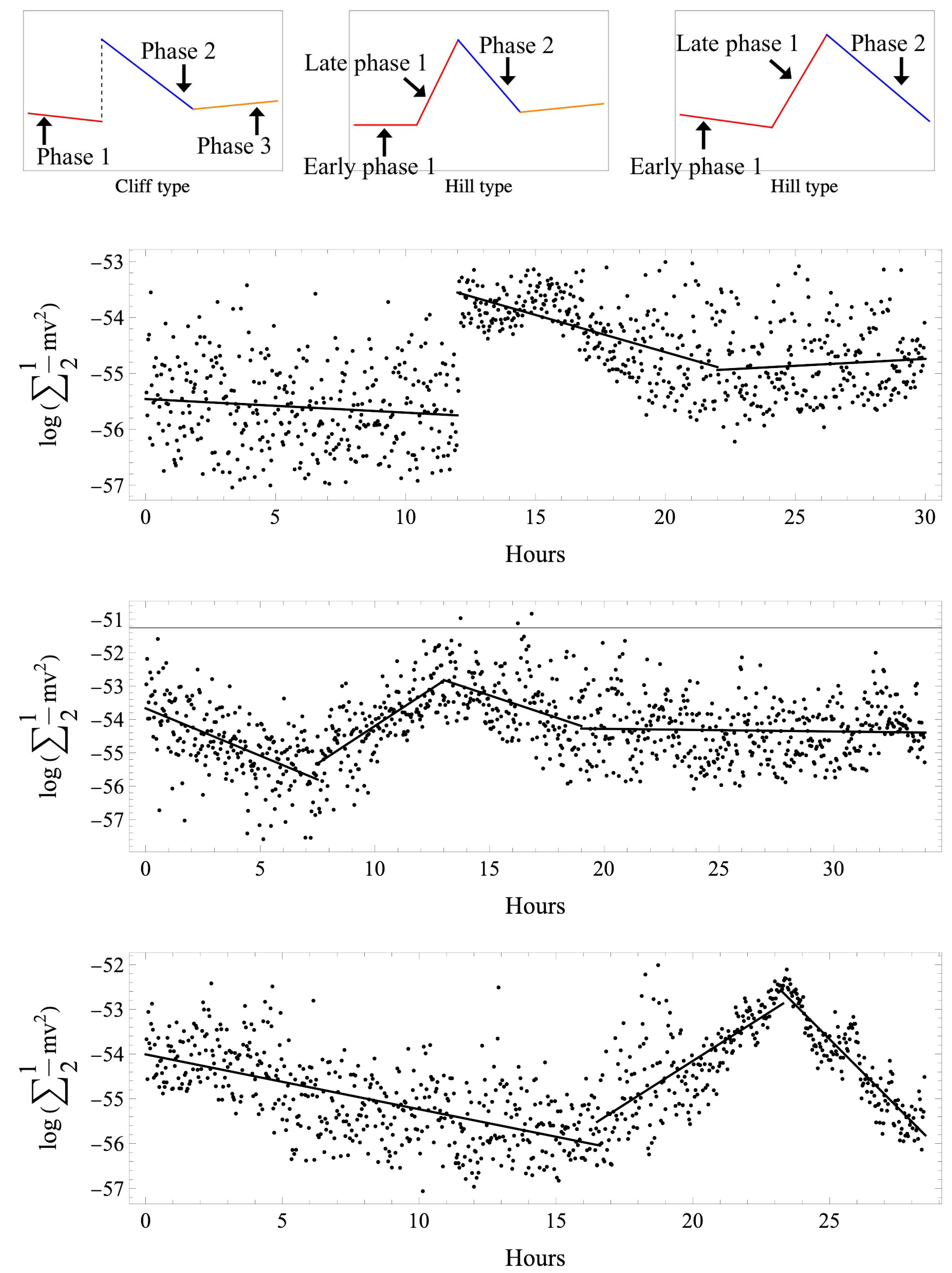
The motion of the particles in the fertilized egg was obtained as a vector, and energy changes over time. Figure 1 shows the samples of the actual profile and scheme, with three types we classified by the profile of the kinetic energy change. All normal cases first showed a slow transition (phase 1), followed by a sudden increase in kinetic energy values mid-transition, resulting in the energy peak that we defined as the start of phase 2, then a gradual decrease (phase 2), and, finally, another slow transition (phase 3). This was defined as the “cliff” type. In addition to the 3 cliff-type cases in the abnormal group, 10 cases were biphasic, with early phase 1 and late phase 1 defined as the “hill” type. The remaining case was a hill type that had moved to first cleavage without phase 3.

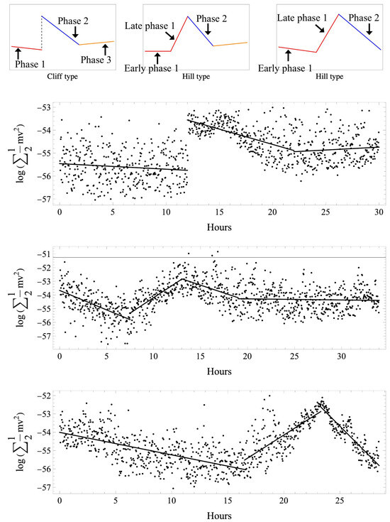
Figure 1. Classification of time variation of the kinetic energy of intracytoplasmic particles in a fertilized egg (top panel). Insemination was defined as the starting point, and analysis was conducted up to the start of the first cleavage. All normal cases first showed a slow transition (phase 1; red line), followed by a sudden increase in kinetic energy values mid-transition, then a gradual decrease (phase 2; blue line), and again a slow transition (phase 3; orange line). This was defined as the cliff type. In addition to the 3 cliff-type cases in the abnormal group, 10 cases were biphasic, with early phase 1 and late phase 1, which were defined as the hill type. The remaining case was a hill type that had moved to first cleavage without phase 3. Actual examples of time variation of kinetic energy and regression lines are shown (lower three panels). The horizontal axis shows the elapsed time after insemination (hours). The vertical axis shows the kinetic energy calculated from norm values (J) and expressed in a logarithm. Cliff-type normal cases (upper panel), hill-type abnormal cases with early and late phase 1 (middle panel), and hill-type abnormal cases with early and late phase 1 but without phase 3 (lower panel) are shown. All normal cases were cliff-type.

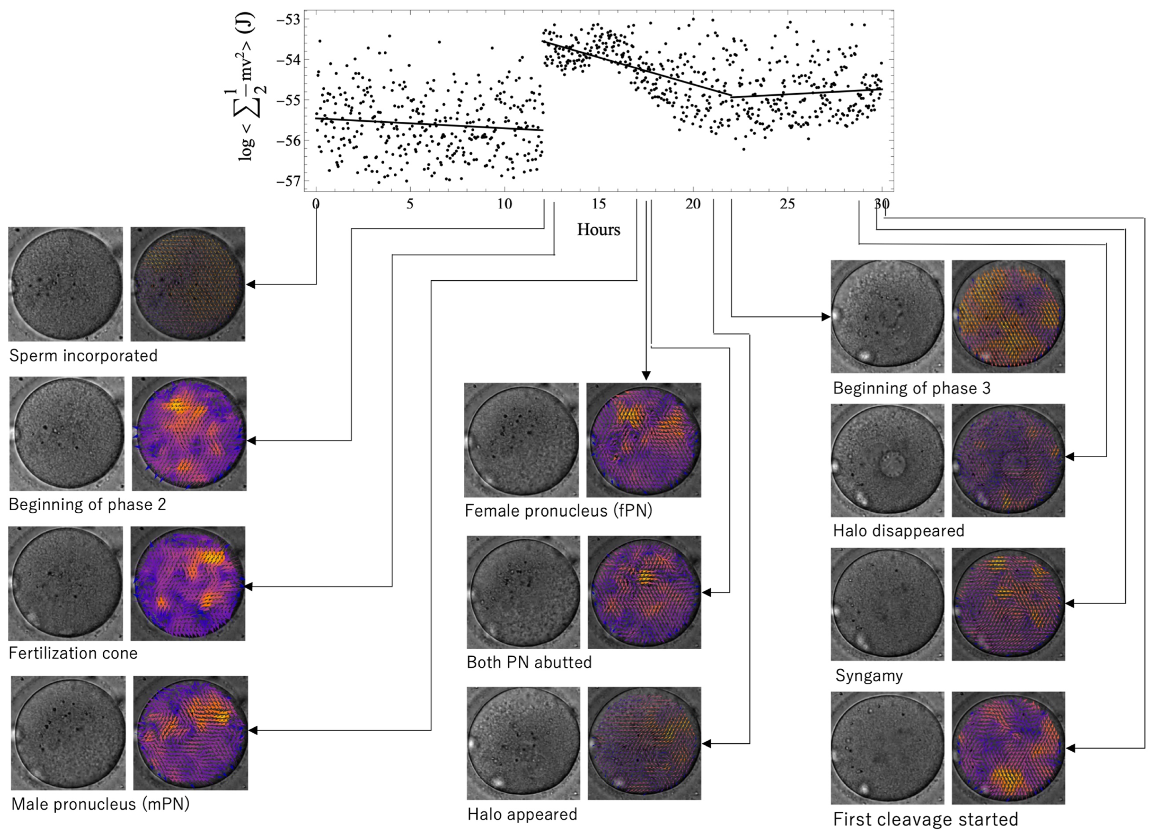
Figure 2 shows the time series evolution of the relationship among morphological characteristics, observed vectors, and kinetic energy values in the normal case. Brighter tones represent larger vectors. The coloration was uneven, and particle movement in the cytoplasm was not uniform. The time when the morphological features were seen did not coincide with the time of energy change, that is, the phase boundary.

Figure 2. The time series evolution of the relationship among morphological characteristics, observed vectors, and kinetic energy values in a normal case. Brighter tones represent larger vectors. The coloration was uneven, and particle movement in the cytoplasm was not uniform. The time when the morphological features were seen did not coincide with the time of energy change; that is, the phase boundary. The fertilization cone, male pronucleus, female pronucleus, and halo appearance emerged during phase 2. PN, pronucleus.

3.1. Analysis in Normal Cases

3.1.1. Time

The transition time (hours) for each phase in normal cases was 7.429 ± 4.201 and 15.543 ± 5.113 (mean ± SD) for phases 1–2 and phases 2–3, respectively, and the time of the first cleavage start was 25.857 ± 6.203 (Table 1, Figure 3). Duration (hours) was 25.771 ± 6.172, 7.429 ± 4.201, 8.114 ± 2.937, and 10.314 ± 3.062, for the entire period and phases 1, 2, and 3, respectively. There were no significant differences in variance or mean among phases 1, 2, and 3, but the mean and median tended to become longer as the phase progressed.

Table 1. Transition duration for each phase in normal and abnormal cases (J). For normal cases, there were no significant differences in variance or mean among phases 1, 2, and 3, but both the mean and median tended to become longer as the phase progressed. For abnormal cases, there was a difference in variance (p = 0.0235) and a significant difference in mean (p = 0.00367) when analyzing five groups: phase 1, early phase 1, late phase 1, phase 2, and phase 3. Analysis of four groups—phase 1, early and late phase 1, phase 2, and phase 3—showed no difference in variance and a significant difference in mean (p = 0.0263), with phase 2 smaller than the other three groups (p < 0.05). Analysis of all three groups (phases 1, 2, and 3) showed no difference in variance and a significant difference in mean (p = 0.0195), with phase 2 smaller than the other two groups (p < 0.05).

	Total	Phase 1	Early Phase 1	Late Phase 1	Phase 2	Phase 3
Normal Case 1	17	8	N/A	N/A	2	7
Normal Case 2	30	12	N/A	N/A	10	8
Normal Case 3	25	2.8	N/A	N/A	11	11.2
Normal Case 4	36	14	N/A	N/A	9.5	12.5
Normal Case 5	21	6.5	N/A	N/A	7.5	7
Normal Case 6	24	4	N/A	N/A	8.5	11.5
Normal Case 7	28	4.7	N/A	N/A	8.3	15
Mean	25.857	7.429	N/A	N/A	8.114	10.314
SD	6.203	4.201	N/A	N/A	2.937	3.062
Q1/4	21	4	N/A	N/A	7.5	7
Med	25	6.5	N/A	N/A	8.5	11.2
Q3/4	30	12	N/A	N/A	10	12.5
Min	17	2.8	N/A	N/A	2	7
Max	36	14	N/A	N/A	11	15
Abnormal Case 8	55.5	33	N/A	N/A	6	16.5
Abnormal Case 9	37	16.5	N/A	N/A	8.5	12
Abnormal Case 10	37.5	4.5	N/A	N/A	6.5	26.5
Abnormal Case 11	28.5	N/A	16.5	6.8	5.2	N/A
Abnormal Case 12	36.5	N/A	15	8	5	8.5
Abnormal Case 13	23.16	N/A	2.5	1.5	0.5	18.66
Abnormal Case 14	20.2	N/A	3	1	1.7	14.5
Abnormal Case 15	34	N/A	7.5	5.5	6	15
Abnormal Case 16	38.5	N/A	8	2.5	21.5	6.5
Abnormal Case 17	35.5	N/A	2	3	4	26.5
Abnormal Case 18	35.7	N/A	4.8	1.4	1.3	28.2
Mean	34.733	18	7.412	3.713	6.018	17.286
SD	9.206	14.309	5.609	2.691	5.685	7.644
Q1/4	28.5	4.5	2.5	1.4	1.7	12
Med	35.7	16.5	4.8	2.5	5.2	15
Q3/4	37.5	33	8	5.5	6.5	26.5
Min	20.2	4.5	2	1	0.5	6.5
Max	55.5	33	16.5	8	21.5	28.2

Med, median; Min, minimum; Max, maximum; N/A, not available; Q1/4, 0.25 quartile; Q3/4, 0.75 quartile; SD, standard deviation.

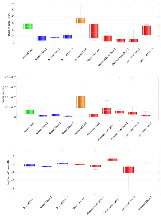
Figure 3. The transition time for each phase in normal and abnormal cases (top panel). For normal cases, duration (hours) was a mean ± standard deviation, median of 25.771 ± 6.172, 25, 7.429 ± 4.201, 6.5, 8.114 ± 2.937, 8.5, and 10.314 ± 3.062, 11.2 for the entire period and phases 1, 2, and 3, respectively. There were no significant differences in variance or mean among phases 1, 2, and 3, but the mean and median tended to become longer as the phase progressed. For abnormal cases, there was a difference in variance (p = 0.0235) and a significant difference in mean (p = 0.00367) when analyzing five groups: phase 1, early phase 1, late phase 1, phase 2, and phase 3. Analysis of four groups—phase 1, early and late phase 1, phase 2, and phase 3—showed no difference in variance and a significant difference in mean (p = 0.0263), with phase 2 smaller than the other three groups (p < 0.05). Analysis of all three groups (phases 1, 2, and 3) showed no difference in variance and a significant difference in mean (p = 0.0195), with phase 2 smaller than the other two groups (p < 0.05).

The average kinetic energy of the intracytoplasmic particles of each phase in the normal case (J) is shown (middle panel). For normal cases, the variance value was higher in phase 1 (p = 0.0065), but there was no significant difference in mean among the phases. For abnormal cases, there was a difference in variance (p = 0.0227) and a significant difference in mean (p = 0.0101). There was a difference in variance (p = 0.0170) and a significant difference in mean (p = 0.000347) among four groups (phase 1, early and late phase 1, phase 2, and phase 3), with early and late phase 1 larger than the other three groups (p < 0.05). There was a variance (p = 0.000263) and a significant difference in mean (p = 0.0138) for all three groups (phases 1, 2, and 3), with phase 1 larger than the other two groups (p < 0.05) and phase 3 smaller (p < 0.05).

The slope ${\beta }_1$ of the regression lines for each phase using the logarithm of the energy value as the objective variable in normal and abnormal cases is shown (lower panel). For normal cases, there was no difference in variance among the phases, but there was a difference in mean (p = 0.0015), and the value of phase 2 was significantly smaller (p < 0.05). For abnormal cases, there was a significant difference in variance among phases (p = 2.325 × 10⁻¹⁰) and a difference in mean (p = 1.454 × 10⁻⁶), with a significantly smaller mean in phase 2 (p < 0.05).

3.1.2. Kinetic Energy Value

Table 2 and Figure 3 show the average kinetic energy of each phase’s intracytoplasmic particles in the normal case. The kinetic energy values (J) were 5.647 × 10⁻²⁴ ± 2.599 × 10⁻²⁴, 2.199 × 10⁻²⁴ ± 2.076 × 10⁻²⁴, 2.369 × 10⁻²⁴ ± 1.255 × 10⁻²⁴, and 1.078 × 10⁻²⁴ ± 4.720 × 10⁻²⁵ for the entire period and phases 1, 2, and 3, respectively. The variance value was higher in phase 1 (p = 0.0065), but there was no significant difference in the means among the phases. The value of $\min F$ was about $1.078\times {10}^{-26}\left(\mathrm{J}\right)$.

Table 2. The average kinetic energy of the intracytoplasmic particles of each phase in normal cases (J). In normal cases, the variance value was higher in phase 1 (p = 0.0065), but there was no significant difference in means among the phases. For abnormal cases, when analyzed among the five groups, there was a difference in variance (p = 0.0227) and a significant difference in mean (p = 0.0101). There was a difference in variance (p = 0.0170) and a significant difference in mean (p = 0.000347) among four groups (phase 1, early and late phase 1, phase 2, and phase 3), with early and late phase 1 larger than the other three groups (p < 0.05). There was a variance (p = 0.000263) and a significant difference in mean (p = 0.0138) for all three groups (phases 1, 2, and 3), with phase 1 larger than the other two groups (p < 0.05) and phase 3 smaller (p < 0.05).

	Total	Phase 1	Early Phase 1	Late Phase 1	Phase 2	Phase 3
Normal Case 1	3.670 × 10−24	2.548 × 10−24	N/A	N/A	6.395 × 10−25	5.083 × 10−25
Normal Case 2	6.304 × 10−24	9.569 × 10−25	N/A	N/A	3.441 × 10−24	1.907 × 10−24
Normal Case 3	3.721 × 10−24	8.320 × 10−25	N/A	N/A	1.932 × 10−24	9.574 × 10−25
Normal Case 4	3.617 × 10−24	1.599 × 10−24	N/A	N/A	1.358 × 10−24	6.595 × 10−25
Normal Case 5	1.053 × 10−24	6.702 × 10−24	N/A	N/A	2.418 × 10−24	1.410 × 10−24
Normal Case 6	4.321 × 10−24	9.727 × 10−25	N/A	N/A	2.405 × 10−24	9.441 × 10−25
Normal Case 7	7.337 × 10−24	1.781 × 10−24	N/A	N/A	4.393 × 10−24	1.163 × 10−24
Mean	5.647 × 10−24	2.199 × 10−24	N/A	N/A	2.369 × 10−24	1.078 × 10−24
SD	2.599 × 10−24	2.076 × 10−24	N/A	N/A	1.255 × 10−24	4.720 × 10−25
Q1/4	3.696 × 10−24	9.570 × 10−25	N/A	N/A	1.358 × 10−24	6.590 × 10−25
Med	4.321 × 10−24	1.599 × 10−24	N/A	N/A	2.405 × 10−24	9.570 × 10−25
Q3/4	7.337 × 10−24	2.548 × 10−24	N/A	N/A	3.441 × 10−24	1.410 × 10−24
Min	3.617 × 10−24	8.320 × 10−25	N/A	N/A	6.390 × 10−25	5.080 × 10−25
Max	1.053 × 10−23	6.702 × 10−24	N/A	N/A	4.393 × 10−24	1.907 × 10−24
Abnormal Case 8	5.404 × 10−24	8.491 × 10−25	N/A	N/A	3.230 × 10−24	1.326 × 10−24
Abnormal Case 9	2.125 × 10−24	3.232 × 10−25	N/A	N/A	1.275 × 10−24	5.266 × 10−25
Abnormal Case 10	9.050 × 10−24	4.444 × 10−24	N/A	N/A	3.161 × 10−24	1.445 × 10−24
Abnormal Case 11	1.145 × 10−23	N/A	1.988 × 10−24	4.733 × 10−24	4.733 × 10−24	N/A
Abnormal Case 12	1.634 × 10−23	N/A	1.031 × 10−23	2.104 × 10−24	2.713 × 10−24	1.219 × 10−24
Abnormal Case 13	1.097 × 10−23	N/A	3.533 × 10−24	3.579 × 10−24	2.784 × 10−24	1.071 × 10−24
Abnormal Case 14	1.985 × 10−23	N/A	8.334 × 10−24	6.963 × 10−24	3.540 × 10−24	1.017 × 10−24
Abnormal Case 15	2.146 × 10−23	N/A	2.990 × 10−24	5.375 × 10−24	9.351 × 10−24	3.745 × 10−24
Abnormal Case 16	3.611 × 10−23	N/A	1.686 × 10−23	6.223 × 10−24	1.122 × 10−23	1.802 × 10−24
Abnormal Case 17	1.958 × 10−23	N/A	5.475 × 10−24	7.603 × 10−24	4.398 × 10−24	2.109 × 10−24
Abnormal Case 18	2.376 × 10−23	N/A	8.234 × 10−24	4.392 × 10−24	5.226 × 10−24	5.910 × 10−24
Mean	1.601 × 10−23	1.872 × 10−24	7.215 × 10−24	5.121 × 10−24	4.694 × 10−24	2.017 × 10−24
SD	9.598 × 10−24	2.243 × 10−24	4.878 × 10−24	1.813 × 10−24	2.997 × 10−24	1.625 × 10−24
Q1/4	9.050 × 10−24	3.232 × 10−25	2.990 × 10−24	3.579 × 10−24	2.784 × 10−24	1.071 × 10−24
Med	1.634 × 10−23	8.491 × 10−25	6.854 × 10−24	5.054 × 10−24	3.540 × 10−24	1.385 × 10−24
Q3/4	2.146 × 10−23	4.444 × 10−24	8.334 × 10−24	6.223 × 10−24	5.226 × 10−24	2.109 × 10−24
Min	2.125 × 10−24	3.232 × 10−25	1.988 × 10−24	2.104 × 10−24	1.275 × 10−24	5.266 × 10−25
Max	3.611 × 10−23	4.444 × 10−24	1.686 × 10−23	7.603 × 10−24	1.122 × 10−23	5.910 × 10−24

Med, median; Min, minimum; Max, maximum; N/A, not available; Q1/4, 0.25 quartile; Q3/4, 0.75 quartile; SD, standard deviation.

3.1.3. Regression Function

A regression line was obtained for each phase using the logarithm of the energy value Y as the objective variable $\widehat{Y}$ with the intercept as ${\beta }_0$ and slope as ${\beta }_1$ (Table 3).

Table 3. Parameters of regression lines obtained for each phase using the logarithm of the energy value Y as the objective variable $\widehat{Y}$ with the intercept as ${\beta }_0$ and slope as ${\beta }_1$. In normal cases, there was no difference in variance between the phases, but there was a difference in mean (p = 0.0015), the value of phase 2 was significantly smaller (p < 0.05), and there was a significant decrease in energy in phase 2 for 100% (7/7) of cases. In abnormal cases, there was a significant difference in variance between phases (p = 2.325 × 10⁻¹⁰) and a difference in mean (p = 1.454 × 10⁻⁶), with a significantly smaller value in phase 2 (p < 0.05).

Case No.	Phase 1			Early Phase 1			Late Phase 1			Phase 2			Phase 3
	Time (H)	${\mathit{\beta }}_0$ ± SE	${\mathit{\beta }}_1$ ± SE	Time (H)	${\mathit{\beta }}_0$ ± SE	${\mathit{\beta }}_1$ ± SE	Time (H)	${\mathit{\beta }}_0$ ± SE	${\mathit{\beta }}_1$ ± SE	Time (H)	${\mathit{\beta }}_0$ ± SE	${\mathit{\beta }}_1$ ± SE	Time (H)	${\mathit{\beta }}_0$ ± SE	${\mathit{\beta }}_1$ ± SE
1	0–8	−52.852 ± 0.090 a	−0.4308 ±0.018 a	N/A	N/A	N/A	N/A	N/A	N/A	8–10	−52.726 ± 1.067 a	−0.352 ± 0.118 c	10–17	−56.724 ± 0.245 a	0.047 ± 0.018 d
2	0–12	−55.458 ± 0.079 a	−0.024 ± 0.011 d	N/A	N/A	N/A	N/A	N/A	N/A	12–22	−51.951 ± 0.187 a	−0.133 ± 0.011 a	22–30	−55.484 ± 0.467 a	0.025 ± 0.018 ¶
3	0–2.8	−56.106 ± 0.224 a	0.024 ± 0.137 ¶	N/A	N/A	N/A	N/A	N/A	N/A	2.8–13.8	−52.810 ± 0.094 a	−0.266 ± 0.010 a	13.8–25	−58.150 ± 0.213 a	0.130 ± 0.011 a
4	0–14	−54.752 ± 0.093 a	−0.084 ± 0.011 a	N/A	N/A	N/A	N/A	N/A	N/A	14–23.5	−51.655 ± 0.291 a	−0.199 ± 0.015 a	23.5–36	−55.681 ± 0.393 a	−0.026 ± 0.013 d
5	0–6.5	−52.722 ± 0.115 a	−0.333 ± 0.030 a	N/A	N/A	N/A	N/A	N/A	N/A	6.5–14	−52.616 ± 0.345 a	−0.249 ± 0.033 a	14–21	−60.091 ± 0.443 a	0.272 ± 0.025 a
6	0–4	−55.562 ± 0.149 a	−0.029 ± 0.064 ¶	N/A	N/A	N/A	N/A	N/A	N/A	4–12.5	−52.871 ± 0.137 a	−0.215 ± 0.016 a	12.5–24	−55.340 ± 0.240 a	−0.017 ± 0.013 ¶
7	0–4.7	−55.157 ± 0.142 a	0.0131 ± 0.053 ¶	N/A	N/A	N/A	N/A	N/A	N/A	4.7–13	−51.222 ± 0.114 a	−0.327 ± 0.012 a	13–28	−56.837 ± 0.169 a	0.064 ± 0.008 a
Mean		−54.659	−0.123								−52.265	−0.249		−56.901	0.070
SD		1.343	0.182								0.653	0.075		1.718	0.103
Q1/4		−55.510	−0.208								−52.768	−0.296		−57.494	0.004
Med		−55.158	−0.029								−52.616	−0.249		−56.724	0.047
Q3/4		−53.803	−0.006								−51.803	−0.207		−55.582	0.097
Min		−56.106	−0.431								−52.871	−0.352		−60.091	−0.026
Max		−52.722	0.024								−51.222	−0.133		−55.340	0.272
8	0–33	−55.808 ± 0.046 a	9.661 × 10−06 ± 0.002 ¶	N/A	N/A	N/A	N/A	N/A	N/A	33–39	−42.949 ± 1.056 a	−0.321 ± 0.029 a	39–55.5	−56.303 ± 0.305 a	0.022 ± 0.006 b
9	0–16.6	−56.949 ± 0.053 a	0.0181 ± 0.006 c	N/A	N/A	N/A	N/A	N/A	N/A	16.5–25	−48.123 ± 0.152 a	−0.352 ± 0.007 a	25–37	−61.593 ± 0.237 a	0.172 ± 0.008 a
10	0–4.5	−53.696 ± 0.101 a	−0.125 ± 0.039 c	N/A	N/A	N/A	N/A	N/A	N/A	4.5–11	−52.283 ± 0.209 a	−0.289 ± 0.026 a	11–37.5	−56.091 ± 0.099 a	0.028 ± 0.004 a
11	N/A	N/A	N/A	0–16.5	−54.008 ± 0.065 a	−0.123 ± 0.007 a	16.5s–23.3	−61.936 ± 0.509 a	0.389 ± 0.025 a	23.3–28.5	−38.327 ± 0.596 a	−0.614 ± 0.023 a		N/A	N/A
12	N/A	N/A	N/A	0–15	−52.3388 ± 0.111 a	−0.244 ± 0.013 a	15–23	−58.327 ± 0.471 a	0.175 ± 0.025 a	23–28	−46.234 ± 0.942 a	−0.328 ± 0.037 a	28–36.5	−55.886 ± 0.592 a	0.013 ± 0.018 ¶
13	N/A	N/A	N/A	0–2.5	−53.892 ± 0.095 a	−0.150 ± 0.064 d	2.5–4	−55.682 ± 0.432 a	0.497 ± 0.133 b	4–4.5	−40.558 ± 2.238 a	−3.260 ± 0.526 a	4.5–23.16	−55.825 ± 0.097 a	0.020 ± 0.007 c
14	N/A	N/A	N/A	0–3	−52.764 ± 0.119 a	−0.418 ± 0.067 a	3–4	−57.628 ± 0.486 a	1.206 ± 0.138 a	4–5.7	−48.509 ± 0.418 a	−1.182 ± 0.086 a	5.7–20.2	−56.184 ± 0.104 a	0.048 ± 0.008 a
15	N/A	N/A	N/A	0–7.5	−53.667 ± 0.120 a	−0.284 ± 0.028 a	7.5–13	−58.697 ± 0.377 a	0.450 ± 0.036 a	13–19	−49.846 ± 0.620 a	−0.229 ± 0.038 a	19–34	−54.126 ± 0.250 a	−0.008 ± 0.009 ¶
16	N/A	N/A	N/A	0–8	−52.209 ± 0.139 a	−0.267 ± 0.030 a	8–10.5	−60.157 ± 1.192 a	0.681 ± 0.128 a	10.5–32	−51.052 ± 0.142 a	−0.125 ± 0.006 a	32–38.5	−60.612 ± 0.845 a	0.158 ± 0.024 a
17	N/A	N/A	N/A	0–2	−53.395 ± 0.258 a	−0.647 ± 0.219 c	2–5	−55.114 ± 0.371 a	0.432 ± 0.103 a	5–9	−50.252 ± 0.367 a	−0.566 ± 0.052 a	9–35.5	−55.198 ± 0.114 a	0.004 ± 0.005 ¶
18	N/A	N/A	N/A	0–4.8	−53.432 ± 0.163 a	−0.091 ± 0.058 ¶	4.8–6.2	−57.645 ± 0.822 a	0.680 ± 0.149 a	6.2–7.5	−45.846 ± 2.410 a	−1.204 ± 0.351 c	7.5–35.7	−54.795 ± 0.127 a	0.022 ± 0.006 a
Mean		−55.484	−0.036		−53.213	−0.278		−58.148	0.564		−46.725	−0.770		−56.661	0.048
SD		1.651	0.078		0.692	0.182		2.221	0.306		4.481	0.902		2.449	0.064
Q1/4		−56.378	−0.063		−53.723	−0.318		−59.062	0.422		−50.049	−0.898		−56.273	0.015
Med		−55.808	9.661 × 10−6		−53.413	−0.255		−57.986	0.474		−48.123	−0.352		−55.989	0.022
Q3/4		−54.752	0.009		−52.658	−0.143		−57.142	0.680		−44.398	−0.305		−55.354	0.043
Min		−56.949	−0.125		−54.008	−0.648		−61.936	0.175		−52.283	−3.260		−61.593	−0.008
Max		−53.696	0.018		−52.209	−0.091		−55.115	1.206		−38.327	−0.125		−54.126	0.172

a, p < 0.0001; b, p < 0.001; c, p < 0.01, d, p < 0.05; Med, median; Min, minimum; Max, maximum; N/A, not available; Q1/4, 0.25 quartile; Q3/4, 0.75 quartile; SE, standard error; SD, standard deviation; ${\beta }_0$, slope; ${\beta }_1$, intercept; ¶ not significant.

The ${\beta }_1$ (J/H) was −0.123 ± 0.182, −0.249 ± 0.075, and 0.070 ± 0.103 (mean ± standard error (SE)) for phases 1, 2, and 3, respectively (Figure 3). There was no difference in variance among the phases, but there was a difference in means (p = 0.0015), and the value of phase 2 was significantly smaller (p < 0.05). In other words, there was a significant decrease in kinetic energy from hyperkinetic energy in phase 2. The kinetic energy value calculated from the regression function rising from the end of phase 1 to the beginning of phase 2 was 4.071 × 10⁻²⁴ ± 3.573 × 10⁻²⁴.

The case-count study results showed that energy in phase 1 decreased in 85.7% (6/7) and increased in 14.3% (1/7) of cases. There was no significant increase in energy in phase 1. There was a significant decrease in energy in phase 2 for 100% (7/7) of cases. Energy in phase 3 increased in 71.4% (5/7) of cases but decreased in 28.6% (2/7) of cases. There was a significant increase in energy in phase 3 for 0 cases, a significant decrease in 14.2% (1/7), and neither a decrease nor an increase in 85.7% (6/7).

3.2. Analysis in Abnormal Cases

3.2.1. Time

Table 1 and Figure 3 show the time required for the entire period, cliff type phase 1, early phase 1, late phase 1, phase 2, and phase 3 in the abnormal cases. Durations (hours) were 34.733 ± 9.206, 18.000 ± 14.309, 7.412 ± 5.609, 3.713 ± 2.691, 6.018 ± 5.685, and 17.286 ± 7.644 (mean ± SD) for the entire period, cliff-type phase 1, early phase 1, late phase 1, phase 2, and phase 3, respectively. Analysis of all three groups (phases 1, 2, and 3) showed no difference in variance and a significant difference in mean (p = 0.0195), with phase 2 smaller than the other two groups (p < 0.05).

3.2.2. Kinetic Energy Value

Table 2 and Figure 3 show the kinetic energies of the entire period, cliff-type phase 1, early phase 1, late phase 1, phase 2, and phase 3 in the abnormal cases. The kinetic energy values (J) were 1.601 × 10⁻²³ ± 9.598 × 10⁻²⁴, 1.872 × 10⁻²⁴ ± 2.243 × 10⁻²⁴, 7.215 × 10⁻²⁴ ± 4.878 × 10⁻²⁴, 5.121 × 10⁻²⁴ ± 1.813 × 10⁻²⁴, 4.694 × 10⁻²⁴ ± 2.997 × 10⁻²⁴, and 2.017 × 10⁻²⁴ ± 1.625 × 10⁻²⁴ (mean ± SD) for the entire period, cliff-type phase 1, early phase 1, late phase 1, phase 2, and phase 3, respectively. There was a variance (p = 0.000263) and a significant difference in mean (p = 0.0138) for all three groups (phases 1, 2, and 3), with phase 1 larger than the other two groups (p < 0.05) and phase 3 smaller (p < 0.05).

3.2.3. Regression Function

Figure 3 shows a graph of the slope ${\beta }_1$ of the regression line for the entire period, cliff-type phase 1, early phase 1, late phase 1, phase 2, and phase 3 in the abnormal cases. Table 3 provides details. ${\beta }_1$, (J/H) was −0.036 ± 0.078, −0.278 ± 0.183, 0.564 ± 0.306, −0.770 ± 0.902, and 0.0479 ±0.064 (mean ± SE) for the entire period, cliff type phase 1, early phase 1, late phase 1, phase 2, and phase 3. There was a significant difference in variance among phases (p = 2.325 × 10⁻¹⁰) and a difference in mean (p = 1.454 × 10⁻⁶), with a significantly smaller value in phase 2 (p < 0.05).

Comparison of Normal and Abnormal Cases

Comparing the overall transit time, the normal and abnormal cases showed 25.857 ± 6.203 and 34.609 ± 9.210 (mean ± SD), respectively. There was no difference in variance between the two groups, with the normal cases reaching first cleavage earlier than the abnormal cases (t-test, p = 0.0425). The total energy values for normal and abnormal cases were 5.647 × 10⁻²⁴ ± 2.599 × 10⁻²⁴ and 1.601 × 10⁻²³ ± 9.598 × 10⁻²⁴, respectively, with a large variance (p = 0.000492) for the abnormal cases. The normal cases tended to have lower total energy values than the abnormal cases, though there was no significant difference (p = 0.124). Comparing the total energy per hour, the normal and abnormal cases were 2.110 × 10⁻²⁵ ± 8.495 × 10⁻²⁶, and 4.989 × 10⁻²⁵ ± 3.017 × 10⁻²⁵, respectively, and the variance significantly differed (p = 0.000742), indicating the total energy per hour was lower in the normal cases than in the abnormal cases (p = 0.0463).

3.3. Comparison of Normal and Abnormal Cases in Phase 2

The time required was 8.114 ± 2.937 and 6.018 ± 5.685 (H) (mean ± SD) for the normal and abnormal groups, respectively, and was greater in the normal group (p = 0.0413). The kinetic energy of phase 2 was 2.369 × 10⁻²⁴ ± 1.255 × 10⁻²⁴, 4.694 × 10⁻²⁴ ± 2.996 × 10⁻²⁴ (J) for the normal and abnormal groups, respectively, and smaller in the normal group (p = 0.0372). ${\beta }_1$ in phase 2 was −0.249 ± 0.075 and −0.770 ± 0.902 (J/H) for the normal and abnormal groups, respectively, with ${\beta }_1$ less in the normal group (p = 0.0372).

3.4. Kinetic Energy and Free Energy Principle

Figure 4 shows an example of the relationship among kinetic energy, sufficient statistics, and free energy calculated every 2 min in phase 2 under certain conditions. As the kinetic energy decreases, the sufficient statistics increase, and the free energy decreases. When sufficient statics are maximized, kinetic energy and free energy are minimized. In phase 2, the change in kinetic energy was considered a sufficient condition for applying the free energy principle.

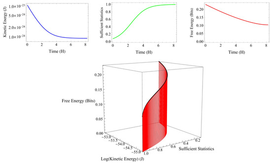
Figure 4. An example of the relationship among kinetic energy, sufficient statistics, and free energy calculated every 2 min in phase 2 under certain conditions (lower panel). As the kinetic energy (blue curve) decreases, the sufficient statics (green curve) increase, and the free energy (red curve) decreases (upper panel). When sufficient statics are maximized, kinetic energy and free energy are minimized. In phase 2, the change in kinetic energy was considered a sufficient condition for applying the free energy principle.

4. Discussion

We have used the free energy principle to explain the biological principle of cytoplasmic dynamics using time-lapse image information. We quantitatively found three phases of kinetic energy change of the particles at the boundary of each elapsed time of 7.429 and 15.543 h in normal cases. Phase 1 is the preparation period for kinetic energy expression, and phase 2 is the period for kinetic energy expression, both of which have almost the same duration. In other words, the time for expression and preparation are almost the same, but the reason for this is unknown. The free energy principle could explain the kinetic energy’s behavior in phase 2, where this energy was most active. The fact that sustained exercise was observed is consistent with the theory that continuous energy consumption is required for stabilizing the adapted state [22].

In phase 2 of normal cases, the kinetic energy value was the largest, though not significant (Table 2, Figure 3), and morphological changes such as male and female pronucleus formation, both pronuclei abutted, and halo appearance were observed. Regarding the clinical significance of the magnitude of kinetic energy and time course in relation to outcome, normal cases reached first cleavage earlier than abnormal cases (p = 0.0425). Kinetic energy profiles showed that all normal cases had a sudden increase in kinetic energy in phase 2, while 27.3% (3/11) of abnormal cases were cliff-type, but 72.7% (8/11) of abnormal cases had a slow transition to phase 2. Total kinetic energy tends to be lower in normal cases. Normal cases have less kinetic energy in phase 2. We considered phase 2 to be the most relevant period. Phase 1 seems to be an energetic preparatory state for phase 2, and when entering phase 2, kinetic energy suddenly rises within 2 min, followed by a gradual decrease to end phase 2. The process then enters phase 3, the final preparatory period for the first cleavage. The biochemical energy metabolism, including thermodynamics, inside the fertilized egg is unknown, but there is probably a major change in the metabolic pathway at the time of the phase 2 transition. In addition to kinetic energy, chemical and thermal energy may be present in the cell, but direct measurement of these energies is extremely difficult because sufficient heat dissipation is required for rapid or accurate development [22].

The findings indicate that when an abnormality in the fertilized egg prevents conception and implantation, the free energy principle theoretically suggests the existence of an abnormality in the generative model generative density, inferential model recognition density, internal observational data of the egg itself, or latent variables originally incorporated in the egg. Specifically, biochemical signal transduction abnormalities correspond to generative model abnormalities, abnormal protein synthesis due to DNA abnormalities and protein production disorders due to ribosomal receptor abnormalities correspond to internal observation data abnormalities, and inborn errors in latent variables are considered to correspond to pathological conditions such as functional abnormalities in which the egg cleavage is not set as recognition density. Therefore, fertilized eggs’ developmental abnormalities could be explained from the viewpoint of the free energy principle. Recently, many embryo evaluation methods using artificial intelligence [23,24,25,26] and estimation of chromosomal aberrations [27,28] have been reported. However, as this research method is in its early stages, the measurement of various parameters related to time and kinetic energy offers potential for prenatal diagnosis, including embryonic development, prediction of live birth, and detection of chromosomal aberrations and genetic abnormalities.

This study does have limitations. The kinetic energy change was largely divided into three phases, though it is possible to further subdivide the time course and interpret that the energy changes up to the first egg cleavage should have more steps. The appropriate image acquisition interval is unknown. In normal cases, the transition to phase 2 occurs within 2 min and should be observed at least every ≤2 min. Second, the relationship between factors possibly associated with particle movement, such as maternal age, maternal complications, information on sperm, chromosomal abnormalities, and genetic abnormalities, needs examining.

The free energy principle has been widely reported in recent years regarding brain function. Though direct free energy measurement is difficult, we were able to estimate the free energy indirectly. The free energy principle, also known as the survival principle of living organisms, was, through this research, suggested as already existing from the moment of birth. The biology of human development encompasses kinetic energy changes and seems to have minimized the developmental system’s informational free energy.

5. Conclusions

The phenomena up to the initiation of the first cleavage in human fertilized eggs are accompanied by dynamic changes in the kinetic energy of cytoplasmic particles. This suggests they may follow the free energy principle. The measurement of kinetic energy while interpreting it in terms of the free energy principle, suggesting clinical usefulness, would further our understanding of the phenomenon of fertilized egg development with respect to the birth of human life. The free energy principle has probably never been discussed in all organisms, not just humans, at the birth of life. Research on the physiological significance of the free energy principle in humans will begin and will be followed by research on its pathological and clinical significance in the future.

References

- Koshland, D.E.; Goldbeter, A.; Stock, J.B. Amplification and adaptation in regulatory and sensory systems. Science 1982, 217, 220–225. [Google Scholar] [CrossRef] [PubMed]
- Ajduk, A.; Ilozue, T.; Windsor, S.; Yu, Y.; Bianka Seres, K.; Bomphrey, R.J.; Tom, B.D.; Swann, K.; Thomas, A.; Graham, C.; et al. Rhythmic actomyosin-driven contractions induced by sperm entry predict mammalian embryo viability. Nat. Commun. 2011, 2, 417. [Google Scholar] [CrossRef] [PubMed]
- Graham, C.F.; Windsor, S.; Ajduk, A.; Trinh, T.; Vincent, A.; Jones, C.; Coward, K.; Kalsi, D.; Zernicka-Goetz, M.; Swann, K.; et al. Dynamic shapes of the zygote and two-cell mouse and human. Biol. Open 2021, 10, bio059013. [Google Scholar] [CrossRef] [PubMed]
- Swann, K.; Windsor, S.; Campbell, K.; Elgmati, K.; Nomikos, M.; Zernicka-Goetz, M.; Amso, N.; Lai, F.A.; Thomas, A.; Graham, C. Phospholipase C-ζ-induced Ca2+ oscillations cause coincident cytoplasmic movements in human oocytes that failed to fertilize after intracytoplasmic sperm injection. Fertil. Steril. 2012, 97, 742–747. [Google Scholar] [CrossRef] [PubMed]
- Milewski, R.; Szpila, M.; Ajduk, A. Dynamics of cytoplasm and cleavage divisions correlates with preimplantation embryo development. Reproduction 2018, 155, 1–14. [Google Scholar] [CrossRef] [PubMed]
- Bui, T.T.H.; Belli, M.; Fassina, L.; Vigone, G.; Merico, V.; Garagna, S.; Zuccotti, M. Cytoplasmic movement profiles of mouse surrounding nucleolus and not-surrounding nucleolus antral oocytes during meiotic resumption. Mol. Reprod. Dev. 2017, 84, 356–362. [Google Scholar] [CrossRef]
- Yi, K.; Unruh, J.R.; Deng, M.; Slaughter, B.D.; Rubinstein, B.; Li, R. Dynamic maintenance of asymmetric meiotic spindle position through Arp2/3-complex-driven cytoplasmic streaming in mouse oocytes. Nat. Cell Biol. 2011, 13, 1252–1258. [Google Scholar] [CrossRef] [PubMed]
- Friston, K.; Kilner, J.; Harrison, L. A free energy principle for the brain. J. Physiol. Paris. 2006, 100, 70–87. [Google Scholar] [CrossRef]
- Friston, K.J. The free-energy principle: A unified brain theory? Nat. Rev. Neurosci. 2010, 11, 127–138. [Google Scholar] [CrossRef]
- Isomura, T.; Shimazaki, H.; Friston, K.J. Canonical neural networks perform active inference. Commun. Biol. 2022, 5, 55. [Google Scholar] [CrossRef]
- Miyagi, Y.; Hata, T.; Miyake, T. Fetal brain activity and the free energy principle. J. Perinat. Med. 2023, 51, 925–931. [Google Scholar] [CrossRef] [PubMed]
- Miyagi, Y.; Hata, T.; Bouno, S.; Koyanagi, A.; Miyake, T. Artificial intelligence to understand fluctuation of fetal brain activity by recognizing facial expressions. Int. J. Gynecol. Obstet. 2023, 161, 877–885. [Google Scholar] [CrossRef] [PubMed]
- Mio, Y. Morphological analysis of human embryonic development using time-lapse cinematography. J. Mamm. Ova Res. 2006, 23, 27–36. [Google Scholar] [CrossRef]
- Mio, Y.; Maeda, K. Time-lapse cinematography of dynamic changes occurring during in vitro development of human embryos. Am. J. Obstet. Gynecol. 2008, 199, 660.e1–660.e5. [Google Scholar] [CrossRef] [PubMed]
- Payne, D.; Flaherty, S.P.; Barry, M.F.; Matthews, C.D. Preliminary observations on polar body extrusion and pronuclear formation in human oocytes using time-lapse video cinematography. Hum. Reprod. 1997, 12, 532–541. [Google Scholar] [CrossRef] [PubMed]
- Horn, B.K.P.; Schunck, B.G. Determining optical flow. Artif. Intell. 1981, 17, 185–203. [Google Scholar] [CrossRef]
- Kyogoku, H.; Kitajima, T.S. Large cytoplasm is linked to the error-prone nature of oocytes. Dev. Cell 2017, 41, 287–298. [Google Scholar] [CrossRef]
- Jarzynski, C. Nonequilibrium equality for free energy differences. Phys. Rev. Lett. 1997, 78, 2690. [Google Scholar] [CrossRef]
- Joyce, J.M. Kullback-Leibler Divergence. In International Encyclopedia of Statistical Science; Lovric, M., Ed.; Springer: Berlin/Heidelberg, Germany, 2011; pp. 720–722. [Google Scholar]
- Inui, T. The free-energy principle: A unified theory of brain functions. Nihon Shinkei Kairo Zassi 2018, 25, 123–134. [Google Scholar] [CrossRef]
- Friston, K.J. The free-energy principle: A rough guide to the brain? Trends Cogn. Sci. 2009, 13, 293–301. [Google Scholar] [CrossRef]
- Lan, G.; Sartori, P.; Neumann, S.; Sourjik, V.; Tu, Y. The energy–speed–accuracy trade-off in sensory adaptation. Nat. Phys. 2012, 8, 422–428. [Google Scholar] [CrossRef]
- Miyagi, Y.; Habara, T.; Hirata, R.; Hayashi, N. New methods for comparing embryo selection methods by applying artificial intelligence: Comparing embryo selection AI for live births. Br. J. Healthc. Med. Res. 2022, 9, 36–44. [Google Scholar]
- Miyagi, Y.; Habara, T.; Hirata, R.; Hayashi, N. Predicting a live birth by artificial intelligence incorporating both the blastocyst image and conventional embryo evaluation parameters. Artif. Intell. Med. Imaging 2020, 1, 94–107. [Google Scholar] [CrossRef]
- Miyagi, Y.; Habara, T.; Hirata, R.; Hayashi, N. Feasibility of deep learning for predicting live birth from a blastocyst image in patients classified by age. Reprod. Med. Biol. 2019, 18, 190–203. [Google Scholar] [CrossRef] [PubMed]
- Miyagi, Y.; Habara, T.; Hirata, R.; Hayashi, N. Feasibility of predicting live birth by combining conventional embryo evaluation with artificial intelligence applied to a blastocyst image in patients classified by age. Reprod. Med. Biol. 2019, 18, 344–356. [Google Scholar] [CrossRef] [PubMed]
- Miyagi, Y.; Habara, T.; Hirata, R.; Hayashi, N. Feasibility of artificial intelligence for predicting live birth without aneuploidy from a blastocyst image. Reprod. Med. Biol. 2019, 18, 204–211. [Google Scholar] [CrossRef]
- Miyagi, Y.; Habara, T.; Hirata, R.; Hayashi, N. Deep Learning to predicting live births and aneuploid miscarriages from images of blastocysts combined with maternal age. Int. J. Bioinfor Intell. Comput. 2022, 1, 10–21. [Google Scholar] [CrossRef]
Disclaimer/Publisher’s Note: The statements, opinions and data contained in all publications are solely those of the individual author(s) and contributor(s) and not of MDPI and/or the editor(s). MDPI and/or the editor(s) disclaim responsibility for any injury to people or property resulting from any ideas, methods, instructions or products referred to in the content. |
© 2024 by the authors. Licensee MDPI, Basel, Switzerland. This article is an open access article distributed under the terms and conditions of the Creative Commons Attribution (CC BY) license (https://creativecommons.org/licenses/by/4.0/).