Numerical Simulation of the Interaction between a Planar Shock Wave and a Cylindrical Bubble

Abstract

Three-dimensional (3D) computational fluid dynamics (CFD) simulations have been carried out to investigate the complex interaction of a planar shock wave (Ma = 1.22) with a cylindrical bubble. The unsteady Reynolds-averaged Navier–Stokes (URANS) approach with a level set coupled with volume of fluid (LSVOF) method has been applied in the present study. The predicted velocities of refracted wave, transmitted wave, upstream interface, downstream interface, jet, and vortex filaments are in very good agreement with the experimental data. The predicted non-dimensional bubble and vortex velocities also have great concordance with the experimental data compared with a simple model of shock-induced Rayleigh–Taylor instability (i.e., Richtmyer–Meshkov instability) and other theoretical models. The simulated changes in the bubble shape and size (length and width) against time agree very well with the experimental results. Comprehensive flow analysis has shown the shock–bubble interaction (SBI) process clearly from the onset of bubble compression up to the formation of vortex filaments, especially elucidating the mechanism on the air–jet formation and its development. It is demonstrated for the first time that turbulence is generated at the early phase of the shock cylindrical bubble interaction process, with the maximum turbulence intensity reaching about 20% around the vortex filament regions at the later phase of the interaction process.

1. Introduction

Shock–bubble interaction (SBI) is an unsteady flow phenomenon created by the shock wave propagation through a distinct round inhomogeneity surrounded by the ambient fluid in an otherwise uniform medium [1]. There are two possible shock refraction patterns when a planar incident shock wave interacts with a gas inhomogeneity: divergent and convergent refraction, depending on the Atwood number (A), defined as follows:

$$A=\frac{{\rho }_2-{\rho }_1}{{\rho }_2+{\rho }_1}$$

(1)

where ${\rho }_1$is the density of the bubble gas and ${\rho }_2$is the density of the ambient gas. When A < 0 (negative), as in the present study, it is referred to as a light bubble case [1,2,3,4]. With respect to the ideal gas speed of sound and at a constant uniform ratio of specific heats, the light bubble case indicates that $c_2$ > $c_1$, where $c_1$ denotes the speed of sound of the ambient unshocked gas while $c_2$ represents the speed of sound of the unshocked bubble gas. Zabusky and Zeng [5] referred to this scenario as the slow-fast-slow, as the speed of sound in the upstream ambient gas is lower (compared with that of the unshocked bubble gas). The speed of sound then increases in the bubble gas and finally reduces within the downstream surrounding gas.

The acoustic impedance $\left(\rho c\right)$ disparity at the interface also represents another method to analyse divergence of shock refraction through the bubble, and SBIs will generally show a divergent ‘light bubble’ refraction feature in the non-uniform-specific heat ratio scenario for ${\rho }_2{c}_2/\left({\rho }_1{c}_1\right)<1$ [1,4,6,7,8,9], where ${\rho }_1$ denotes the density of the ambient unshocked gas while ${\rho }_2$ represents the density of the unshocked bubble gas. For the case where ${\rho }_2{c}_2/\left({\rho }_1{c}_1\right)<1$ at the interface and at small angles of incidence, the regular refraction happens where the transmitted wave and incident wave meet the interface at the same point while irregular refraction patterns are observed at higher angles [10,11]. SBI is also characterised by nonlinear acoustic impacts, which deal with refraction, reflection, and diffraction of the incident shock wave by the bubble. This process also involves a subsequent change in the shape and motion configuration of the shock wave by the bubble attributable to the interface curvature and disparity of the acoustic impedance.

Many studies have been carried out to investigate shock cylindrical bubble interaction experimentally and numerically. Rudinger and Somers [12] investigated the behaviour of cylindrical gas bubbles in accelerated flows experimentally and theoretically. Their theoretical model shows that the ratio of the bubble velocity to the ambient gas velocity is dependent on the density ratio of the two gases as well as the bubble shape. Their experimental results, using hydrogen (H₂), helium (He), and sulphur hexafluoride (SF₆), accelerated by varying the strength of shock waves, are in good concordance with the theoretical predictions. Jacobs [7,8] experimentally investigated the distortion of a helium cylinder by a weak shock wave through the planar laser-induced fluorescence (PLIF) for flow visualisation instead of using shadowgraphs. There was a good agreement between their results and the past experimental/computational results with respect to the deformation of the helium cylinder induced by the propagating shock wave, and their work showed that a rapid mixing occurred due to the vorticity-induced motion. Ding et al. [13] performed experimental and numerical studies of the interaction of a planar shock wave with two-dimensional (2D) and three-dimensional (3D) nitrogen-filled cylinders surrounded by sulphur hexafluoride (SF₆). Their research highlighted the impacts of the initial interface curvature on flow morphology, wave pattern, distribution of vorticity, and interface movement. Their numerical research combined the high-order weighted essentially non-oscillatory construction with the double-flux scheme to study the detailed 3D flow structures. Their results showed that at very preliminary phases of SBI, pressure oscillations in the evolving interface area stimulated by complex waves contribute significantly to the 3D gas cylinder’s distortion. However, following shock propagation through the cylinder, baroclinic vorticity deposited at the gas cylinder controls the deformation of the interface.

Piccone and Boris [14] performed the first comprehensive numerical study of SBI in 2D simulations following the experiments performed by Haas and Sturtevant [6] for spherical and cylindrical bubbles. Even though their 2D simulations only had a grid resolution of fewer than 50 cells per bubble radius (R50), they still managed to represent the evolution of the vortical features observed by Haas and Sturtevant [6]. Quirk and Karni [15] described a comprehensive numerical investigation of SBI using a sophisticated adaptive mesh refined algorithm with a non-conservative shock-capturing scheme. The adaptive mesh refinement technique allowed them to yield outcomes with high resolution at a low computational cost, and there was an effective resolution of the shock refraction pattern and vortical features noticed by Haas and Sturtevant [6]. Bagabir and Drikakis [16] investigated the impact of the strength of the incident shock on the cylindrical bubble behaviour with similar characteristics as in the experiments conducted by Haas and Sturtevant [6]. Their simulations used the Euler equations, together with a high-resolution Godunov-type method and an implicit solver, for various incident shock Ma. Their simulations revealed, at higher Ma, extra gas dynamic characteristics like the secondary-reflected shock and circular-shaped structure as opposed to the ‘c-shaped’ structure observed at lower Ma. Marquina and Mulet [9] simulated the experiments of Haas and Sturtevant [6], utilising a conservative extension of the Euler equations (solved using a flux-split algorithm in conjunction with a high-order (WENO5) flux reconstruction to decrease the oscillations in the vicinity of the air–gas interface) and a very high spatial resolution. The results revealed the evolution of distinctive turbulent features in the flow field during delayed timescales. Taniguchi et al. [17] used an advanced volume of fluid (VOF) technique called the non-uniform sub-cell scheme (NSS) [18], which helped to track a sharp interface for an extended duration whilst ensuring conservation of mass. They also adopted the total variation diminishing (TVD) scheme [19] to capture the shock waves. Their results showed that the proposed method could predict the 2D interaction of a shock wave interacting with an air–gas interface accurately. Wang et al. [20] numerically investigated the vortex breakdown behaviour of the scaling criterion in the interaction between an incident shock and a cylindrical bubble, showing the appearance of a vortex breakdown in terms of bubble morphology and interface stretching. Chen et al. [21] numerically studied the interaction of shock waves with circular or elliptic bubbles in an air medium. They used a five-equation model and the finite volume method (FVM) to numerically examine the generation/distribution of vorticity as well as its impact on the bubble interface deformation and turbulent mixing acceleration of the two-phase gas. Singh et al. [22] numerically studied the effect of bulk viscosity on flow morphology of shock-accelerated cylindrical light bubbles in both diatomic and polyatomic gases. They adopted an explicit mixed-type modal discontinuous Galerkin scheme with the uniform meshes to solve a 2D system of unsteady physical conservation laws. They compared their results with monoatomic gases and elucidated that diatomic and polyatomic gases produce bigger rolled-up vortex chains, different inward jet formations, and sizeable mixing zones with intense large-scale expansion.

The aforementioned numerical investigations are mainly 2D, and so far, not many fully 3D numerical studies have been performed. Our current understanding of the SBI process is far from complete, especially on the generation/development of turbulence that has not been addressed previously. The main objective of the present study is to advance our current understanding of the shock–cylindrical bubble interaction process through a detailed 3D simulation, especially on the generation and development of turbulence as well as the evolution of vortex filaments.

This paper is structured as follows: the methodology employed for this study is described in Section 2, including the governing equations and numerical methods, computational details, and mesh independence study. Section 3 presents both quantitative and qualitative comparisons between the numerical predictions and measured experimental data as well as a comprehensive analysis of the instantaneous flow fields to elucidate the SBI process. Section 4 draws the concluding remarks.

2. Methodology

2.1. Governing Equations

The fundamental governing equations (Navier–Stokes equations) based on the conservation of mass, momentum, and energy are standard equations, which can be found in many textbooks and papers and hence will not be presented here again. SBI is predominantly unsteady, and turbulence is generated at the later stage of SBI with usually large-scale unsteady flow structures. It was demonstrated by Onwuegbu and Yang [23] that for this kind of flow, the unsteady Reynolds-averaged Navier–Stokes (URANS) approach could predict the flow accurately at a significantly reduced cost so that there was no need in using two other more accurate approaches, i.e., large-eddy simulation (LES) and direct numerical simulation (DNS). The URANS equations are obtained by averaging the fundamental governing equations, leading to some extra terms called Reynolds stresses being generated due to the averaging process. Those terms needed to be approximated (modelled) using a turbulence model; otherwise, the number of unknowns is more than the number of equations. There are many turbulence models available, and the selection of an appropriate turbulence model for this study is presented in Section 2.6.

2.2. Level Set Coupled with Volume of Fluid

One-fluid formulation with an interface capturing approach has been adopted in the present study. An accurate interface tracking technique is hence required to capture the bubble deformation properly. Several methods are available to track the interface, but most of them struggle to handle large interface distortions, i.e., disintegration and fronts fusing [24]. Our previous study of a shock–spherical bubble interaction [23] showed that a level set coupled with volume of fluids (LSVOF) model would be able to capture the bubble deformation accurately. Two transport equations need to be solved in the LSVOF approach, one for the level set and one for the volume fraction. The level set (LS) method, which is a popular interface-tracking method for computing two-phase flows with topologically complex interfaces, captures and tracks the interface by the level-set function specified as a signed distance from the interface [25]. However, the level-set method suffers from a deficiency in volume conservation preservation [26]. The VOF, on the other hand, can preserve volume conservation, as it calculates and tracks the volume fraction of a particular phase in each cell instead of the interface itself. However, the computation of the spatial derivatives for the VOF method poses a challenge, as the volume fraction of a particular phase is not continuous across the interface. The LSVOF enables the added sophistication of automatically treating topological alterations with a higher accuracy than the standalone LS and VOF models, as it combines their merits and overcomes their deficiencies. Thus, LSVOF offers the benefits of being discretely conservative at the air–helium bubble interface and also correctly predicting the position of the interface and the shockwaves.

In the present study, a transport equation for the volume fraction of helium takes the following simpler form without any source terms on the right-hand side since there is no mass transfer between air and helium.

$$\frac{\partial {\alpha }_h}{\partial t}+\nabla ·\left({\alpha }_h\overrightarrow{V}\right)=0$$

(2)

where ${\alpha }_h$is the volume fraction of helium, and the volume fraction of air can be computed from the following equation:

$${\alpha }_h+{\alpha }_a=0$$

(3)

The density and viscosity in each cell are calculated based on the volume fraction:

$$\rho ={\alpha }_h{\rho }_h+{\alpha }_a{\rho }_a \mu ={\alpha }_h{\mu }_h+{\alpha }_a{\mu }_a$$

(4)

A single momentum is solved in the present study with the resulted velocity shared by both air and helium.

2.3. Spatial and Temporal Discretisation

A third-order monotone upstream-centered schemes for conservation laws (MUSCL) without a slope limiter has been employed for spatial discretisation. This scheme was introduced by Van Leer [27] based on the original MUSCL by blending a central differencing scheme and second-order upwind scheme.

A first-order implicit scheme has been used for the temporal discretisation. To achieve numerical stability (the Courant–Friedrichs–Lewy number was set as 0.5) and accuracy; a very small-time step of $4\times {10}^{-7}$seconds has been used in the present study.

2.4. Computational Details

The computational set-up replicates the experiment carried out by Haas and Sturtevant [6] with the key parameters shown in

Table 1. Experimental conditions.

Bubble Gas	Helium
Ambient gas	Air
Ma number	1.22
Atwood number	−0.715

.

Figure 1 shows the computational domain, where the $x$-axis is horizontal, the $y$-axis is vertical, and the $z$-axis is spanwise. The length of the computational domain is 5d and both the height and width are 2d (d is the bubble diameter, 50 mm, used in the experiment of Haas and Sturtevant [6]). The domain length has been selected to provide enough space for the shocked bubble to travel throughout the monitored time. The no-slip boundary condition is employed on the top, bottom, and side walls. At the outlet boundary, a zero gradient boundary condition is used for all the variables. At inlet, the horizontal velocity component is 115 m/s, and both the vertical and spanwise velocity components are zero, pressure is 263,325 Pa, and density is 1.8 kg/m³. The initial values in the rest of the computational domain are as follows: velocity is zero, pressure is 101,325 Pa both inside and outside the bubble, air density is 1.29 kg/m³, and helium density inside the bubble is 0.214 kg/m³. It is worth pointing out that in the experiment [6], there existed a finite-thickness interfacial transition layer at the initial interface, while in the simulations, a sharp interface with the interface discontinuities was used. Furthermore, a nitrocellulose membrane was used with a slight overpressure in the cylinder to form the initial interface in the experiment [6]. This introduces additional surface and viscous forces on the interface, whereas no additional forces were introduced in the simulations.

The computational mesh shown in Figure 2a,b mainly consists of structured mesh, while unstructured mesh is employed in the vicinity of the bubble (both inside and outside). The unstructured cells used in the bubble vicinity enable the local alignment of the grid orientation to the dominant flow direction due to their flexible nature, thus lessening numerical diffusion [28], and have been validated by the works of previous researchers [28,29]. The Cartesian cut-cell method, previously applied by Ingram et al. [30] and Johnson [31], has been used to produce this mesh to make sure that a high-quality mesh can be generated in the bubble vicinity.

Adaptive mesh refinement (AMR) helps to generate a more robust high-resolution grid capable of reproducing a sharp representation of discontinuities and also sufficiently resolving the various flow structures to be investigated. AMR thus ensures that the mesh is refined inside the bubble and its vicinity (including the primary shock wave), guaranteeing that the fine cells surround and travel with the bubble to provide for the strong interaction between the incident shock waves and the bubble.

2.5. Mesh Independence Study

A mesh independence study has been performed with three meshes (4.5, 5.8, and 9.5 × 10⁶ cells) to ensure that the predictions are independent of the mesh size. Figure 3 shows the bubble evolution with time using three representative positions, i.e., upstream, jet, and downstream locations. From Figure 3, the predicted results from all three meshes show little variation, but mesh-independent results are not really achieved. Hence the experimental data are added to Figure 3, which shows that with the increasing grid number, the predictions monotonically approach the experimental data [6] so that the mesh with 9.5 M elements would be the best for this study.

2.6. Turbulence Model Selection

Many turbulence models have been developed, but selecting a suitable model is quite difficult since their performances are often case dependent. In the present study, three widely used and highly rated models were tested: the realisable k-ε, the shear stress transport (SST) k-ω, and a Reynolds stress model (RSM). Figure 4 shows the comparison between the predicted results and the experimental data [6]. Inviscid simulations were also performed and presented in Figure 4. It is clear from Figure 4 that initially all the predictions are more or less the same, and as the flow develops with time, the predictions using all three turbulence models show a better agreement with the experimental measurements of Haas and Sturtevant [6] than the inviscid predictions. This indicates that turbulence is generated after the shock interacts with the bubble, and turbulence modelling is needed in order to obtain accurate results. Furthermore, the predictions using all three turbulence models show little disparity, but the results obtained using the realisable k-ε model are very slightly closer to the experimental data. Therefore, the realisable k-ε turbulence model has been used in this study.

3. Results

3.1. Comparison between the Measured and Predicted Velocities

Table 2. Comparison between the predictions and the experimental data [6] (velocity unit: $\mathrm{m}/\mathrm{s}$).

	Experimental Data	Current Study
$u_I$	410	403.3
$u_R$	900	894.6
$u_T$	393	388.8
$u_{IU}$	170	166.5
$u_{FU}$	113	110
$u_{ID}$	145	141.3
$u_{AJ}$	230	2226.7
$u_f$	128	122.2

below presents the comparison between the measured and predicted velocities of incident ($u_I$), refracted ($u_R$), and transmitted waves ($u_T$), as well as the different characteristic interface points, i.e., initial upstream interface ($u_{IU}$), final upstream interface ($u_{FU}$), initial downstream interface ($u_{ID}$), air-jet head ($u_{AJ}$), and vortex filament ($u_f$). The velocities of these acoustic wave characteristics are obtained by using minimum squares line adjustments to estimate their approximate locations, at different times, along the bubble trajectory. It is evident from Table 2 that there is an excellent agreement between the numerical predictions and the experimental data for all the derived velocities, with the maximum error being about 3% for the final upstream interface velocity.

3.2. Air Displacement, Bubble Acceleration, and Vortex Formation

Air is accelerated in the shock tube during the shock wave propagation, from a state of rest to a uniform velocity, $U_2$:

$$U_2=\frac{2a_0}{\gamma +1}\left(M{a}_1-\frac{1}{M{a}_1}\right)$$

(5)

As helium is less dense than air, the cylinder containing helium will be accelerated to a larger velocity than $U_2$, and the flow behind the incident shock acts as a piston on the bubble, thus leading to the bubble deformation and compression. This then means that the light helium gas travels ahead of the ambient air as it is propagated down the shock tube following the incident shock wave. Even though helium bubble initially translates as a solid cylinder, it eventually yields to the forces induced by the propagation of the ambient air. This is what leads to the formation of the vortex filament pair.

Rudinger and Somers [12] presented a simple two-phase model of SBI in which throughout the early transients, the bubble accelerates as a solid body to a velocity of $U_b$ and is transformed into a vortex ring with a velocity of $U_v$ in the final evolution phase, following Taylor’s mechanism [32]. The travelling, undistorted bubble during the first phase functions as Taylor’s ‘undissolved’ vortex-generating disk such that $U_b$ represents the disk velocity. Rudinger and Somers [12] proposed that the impulse per unit volume undergone by the bubble, $I_b$, would equal that underwent by the ambient air, i.e., ${\rho }_{air}\times U_2$, where ${\rho }_{air}$ denotes the ambient gas density. Mathematically, this is shown below:

$$I_b={\rho }_a \times U_2={\rho }_h{U}_b+k{\rho }_a\left(U_b-U_2\right)$$

(6)

where $k$ represents the apparent mass fraction for a cylinder, which is equal to 1.0, ${\rho }_h$ denotes the bubble gas density, and ${\rho }_a$is the air density. From Equation (6), the initial non-dimensional bubble velocity is then calculated as:

$$U_{N{D}_b}=\frac{U_b}{U_2}=\frac{1+k}{\sigma +k}$$

(7)

where $\sigma$ = ${\rho }_h/{\rho }_a$.

The conversion of the bubble into a vortex implies a drop in the relative velocity, as shown below:

$$U_v-U_2=\beta \left(U_b-U_2\right)$$

(8)

where $\beta$ has a numerical value of 0.203 for the cylinder as computed by Rudinger and Somer [12].

From Equation (8), the non-dimensional vortex velocity can be calculated as:

$$U_{N{D}_v}=\frac{U_v}{U_2}=1+\beta \frac{1-\sigma }{\sigma +k}$$

(9)

Just as in the experimental works of Haas and Sturtevant [6], $U_b$ is obtained as the average of the predicted initial upstream and downstream interface velocities $u_{IU}$ and $u_{ID}$ from Table 2. $U_v$ is obtained as $u_f$ from Table 2. The predicted, theoretical, and measured values for those two non-dimensional velocities are presented in

Table 3. Theoretical, numerical, and experimental non-dimensional bubble and vortex velocities.

	Theoretical Values	Experimental Data	Current Study
$U_{N{D}_b}$	1.692	1.37	1.345
$U_{N{D}_v}$	1.14	1.12	1.068

.

Table 3 shows that the predicted initial non-dimensional bubble velocity agrees very well with the experimental data, while the theoretical value is far too large. Nevertheless, for the non-dimensional vortex velocity, the theoretical value is slightly closer to the experimental data than the current prediction, indicating that the theoretical model could capture the vortex formation reasonably well but not the bubble acceleration. It is demonstrated that the complete process of bubble acceleration and vortex formation are well captured by the current simulations.

3.3. Distortion and Evolution of the Interface

Figure 5 presents the comparison between the predicted dimensionless displacement of the upstream interface $(y_{ups}/d)$ and the experimental data [6] plus the previous numerical results by Chen et al. [21]. It can be seen clearly that a very good agreement between the current predictions and the experimental data has been obtained for the whole process, while the numerical results by Chen et al. [21] start to divert away from both experimental data and the current predictions after the first 125 μs.

Figure 6 shows the predicted dimensionless displacement of the downstream interface $(y_{downs}/d)$ with time compared with the experimental data [6] and the numerical results of Wang et al. [20]. It can be seen clearly that the current predictions show a very good agreement with the experimental data. It is also observable that the current study provides slight underpredictions of the displacement, while the previous numerical study overpredicted the displacement slightly.

Figure 7 presents the predicted and measured location changes of the bubble with time at the three characteristic interface points. As shown in Figure 8, the predictions match the experimental data [6] extremely well.

It is evident from the above quantitative comparisons between the predictions and experimental data that the simulations have captured the complex shock–bubble interaction accurately. Further qualitative analysis will be presented below to elucidate the complex shock–bubble interaction process, leading to a better understanding of the process.

3.4. Shock–Bubble Interaction Process on a 2D Plane

The intricate and crucial processes involved in the bubble deformation, generation of vorticity, growth of the air-jet, and the overall development of the SBI process will be further elucidated in this section. Figure 8 presents eight snapshots of the simulated images (right) on the central x-y plane and shadow-photographs (left) captured in the experiment. The dimensionless time, t, is normalised by the shock velocity and the diameter of the bubble, and t = 0 corresponds to the instant when the incidence shock impinges the upstream end of the bubble. In Figure 8, $ue$, $de$, $aj$, $hbs$, and $vf$ represent the upstream interface, downstream interface, air-jet, helium bridge structure, and vortex filament. It is evident from Figure 8 that the simulated images are quite similar to the shadow-photographs [6] at all those eight instants. This demonstrates that the predictions capture the SBI process very well, reproducing all the major characteristics observed in the experiment [6]. Figure 8a shows the helium cylindrical bubble at $t$ = 0.34 following the incident shock wave ($iw$) impingement on the upstream side of the helium volume from the right-hand-side. The $iw$ is seen as two straight branches connected at the top and bottom of the bubble interface to the curved refracted wave ($rs$) travelling inside the bubble and to the reflected wave ($rfw$) travelling outside the bubble. Figure 8b ($t$ = 0.51) reveals the $rs$ travelling further forward and faster than the $iw$ (because the sound velocity of the helium bubble is greater than that of air). The $rs$ is connected to the two branches of the primary transmitted wave, $pts$, at the top/bottom of the bubble, and the $pts$ intersect the two branches of the $iw$. At $t$ = 0.6, there is a complete emergence of the $pts$ from the downstream end of the bubble, coupled with the appearance of the converging internal reflected wave ($irw$), as shown in Figure 8c. The simulated image in Figure 8d at $t$ = 0.85 shows that the $irw$ has developed into a diverging wave (not very visible from experiments) after propagating across its caustic. The continuous compression of the upstream interface means the cylindrical bubble distortion persists, and at $t$ = 2.11, the deformed helium bubble has attained a kidney shape and the $aj$ starts to form, as seen in Figure 8e. It can be seen from Figure 8f,g at $t$ = 3.88 and $t$ = 5.74, respectively, the $aj$ develops through the bubble centre, and a spike forms behind the jet. The magnitude of the velocity arriving at the bubble centre becomes progressively greater. Although the bubble is severely distorted up to $t$ = 5.74, the $aj$ has not completely penetrated the bubble. Due to the interfacial density mismatch, the pressure on the upstream end of the bubble increases with the $aj$. This makes the lighter helium push against the heavier air, causing the top and bottom ends of the upstream interface to move up and the middle end of the upstream interface (area through which $aj$ pushes through) to move down. This movement leads to a caving of the upstream interface through the centre, leading to the formation of $hbs$ and $vf$, as shown in Figure 8g. At $t$ = 8.44, the experimental shadow-photograph in Figure 8h shows that the bubble has been more or less smashed, and $hbs$ and $vf$ are not visible anymore, while in the simulated image, the $aj$ is about to penetrate the bubble completely, and $hbs$ and $vf$ are still clearly visible. Furthermore, it is clear from the experimental shadow-photograph in Figure 8h that small flow structures have been formed, especially at the bottom half, indicating that turbulence is already developed, which will be further discussed in Section 3.7.

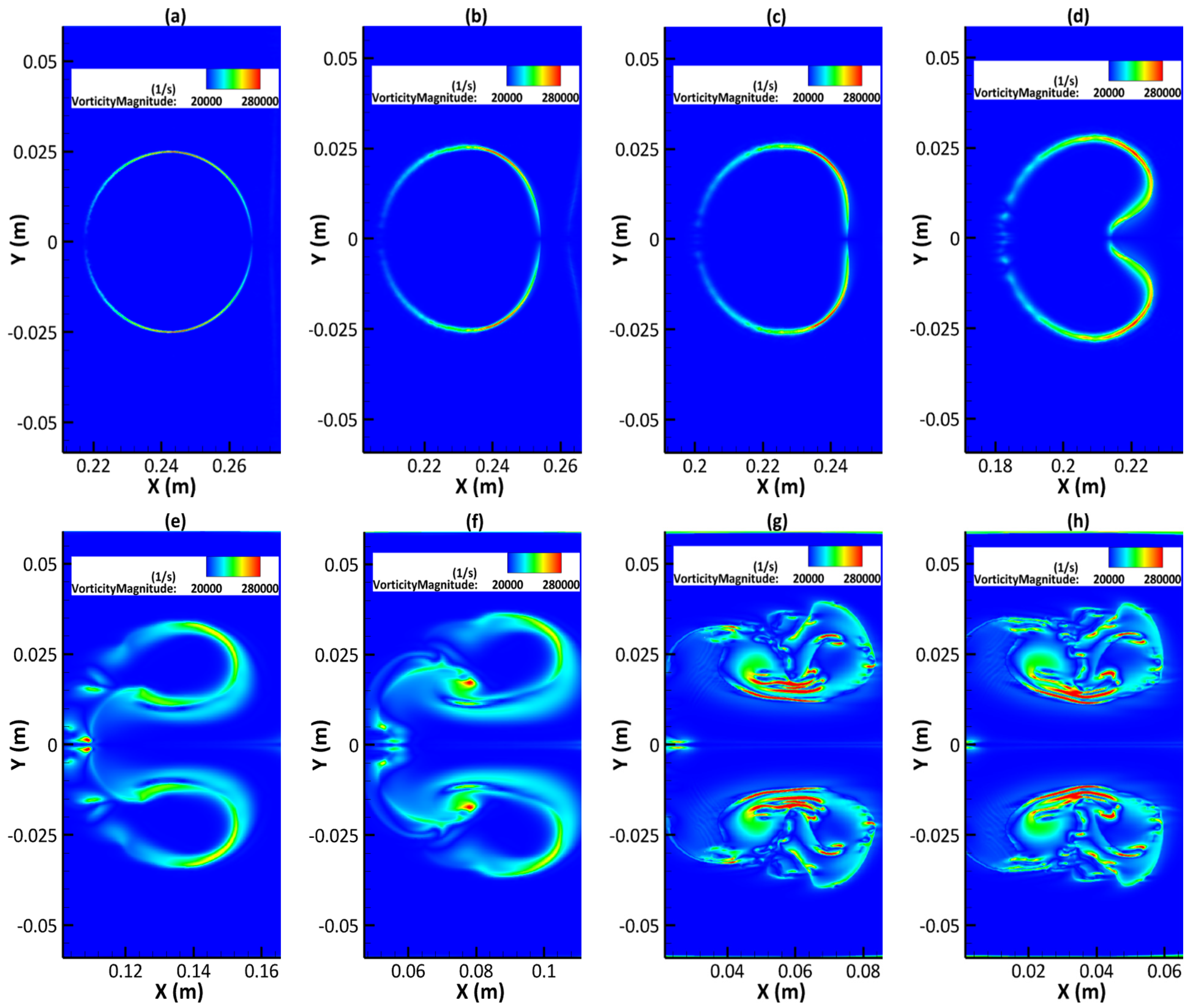
3.5. Vorticity Generation

One of the most essential phases of SBI is the vorticity generation and deposition due to the disparity between the pressure and density gradients. As the shock waves (incident, refracted, diffracted, and focused waves) propagate through the bubble, vorticity is generated and transported in the flow. Vorticity is so essential in SBI as it, together with aerodynamic forces, principally influences the motion and structure of the bubble [2].

Figure 9 shows contours of the vorticity magnitude on the central x-y plane at different stages of the SBI process. At the early stage, as shown in Figure 9a–d, vorticity is produced around the air–helium interface (bubble surface) as a result of flow baroclinity, i.e., due to the misalignment of the local pressure gradient from the density gradient, and the air-jet formation can be clearly seen in Figure 9d. Figure 9e at $t$ = 3.88 shows that the air-jet is about to reach the downstream interface, and the upstream interface is severely distorted, with more vorticity generated around the interface region. At $t$ = 5.74, the air-jet reaches the downstream interface, as shown in Figure 9f, and a pair of vortex filaments ($vf$) is clearly observed, with high vorticity concentrated in the vortex filament region. As time passes by, more vorticity is generated around the $vf$ region and the surrounding regions, as shown in Figure 9g,h. Small flow structures can also be observed at the later stages of the SBI process. This strongly suggests that vorticity, generated by baroclinic mechanism, plays a very important role in the SBI process, i.e., it initiates the deformation of the upstream surface, and afterwards, strong rotational motions are produced, which pull a jet of ambient air through the centre of the bubble. The jet deforms the bubbles until it pierces the downstream bubble interface. Vortices at the bubble surface roll up and drag helium into a distinctive downstream $vf$ pair, as shown in Figure 9f–h.

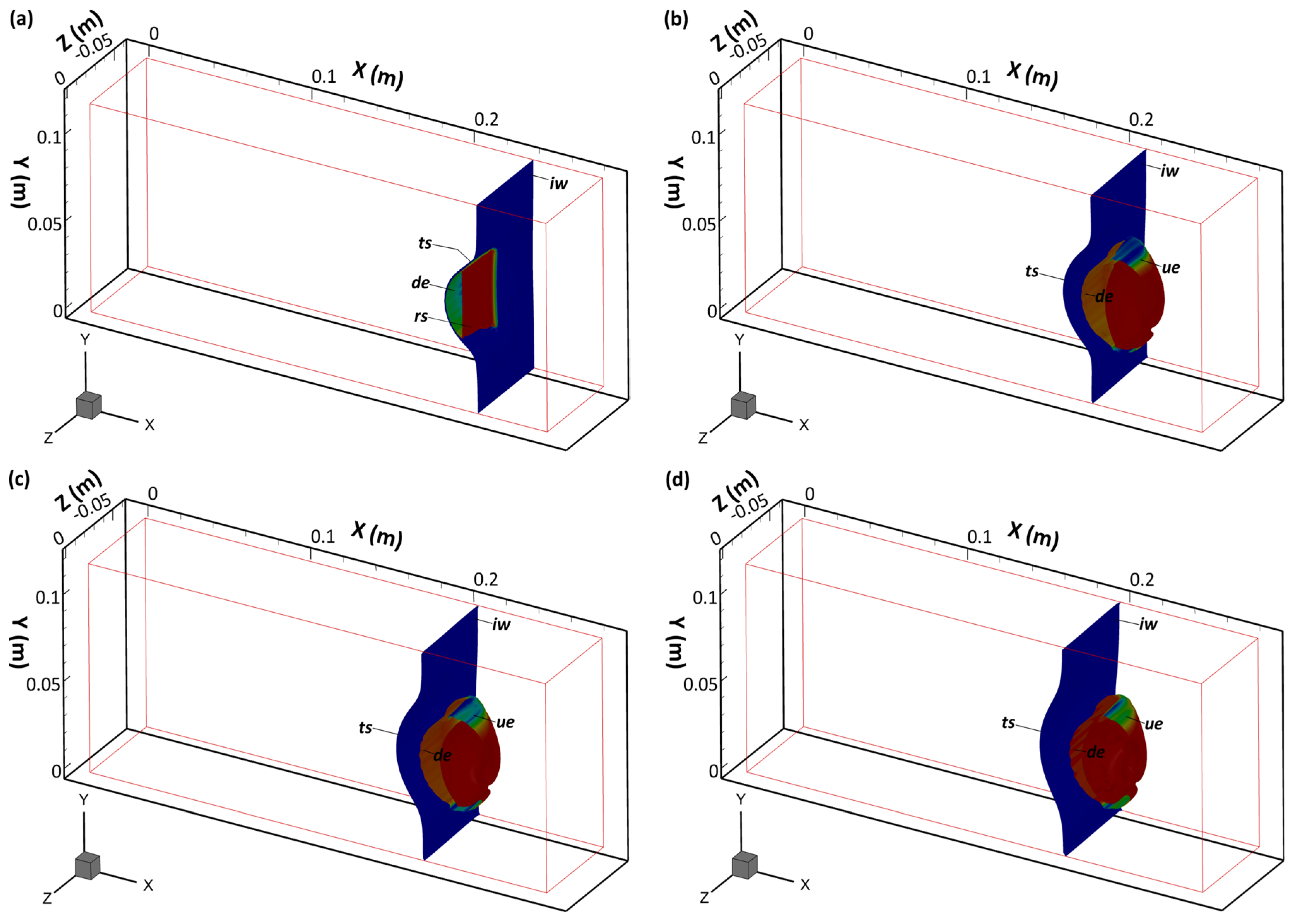
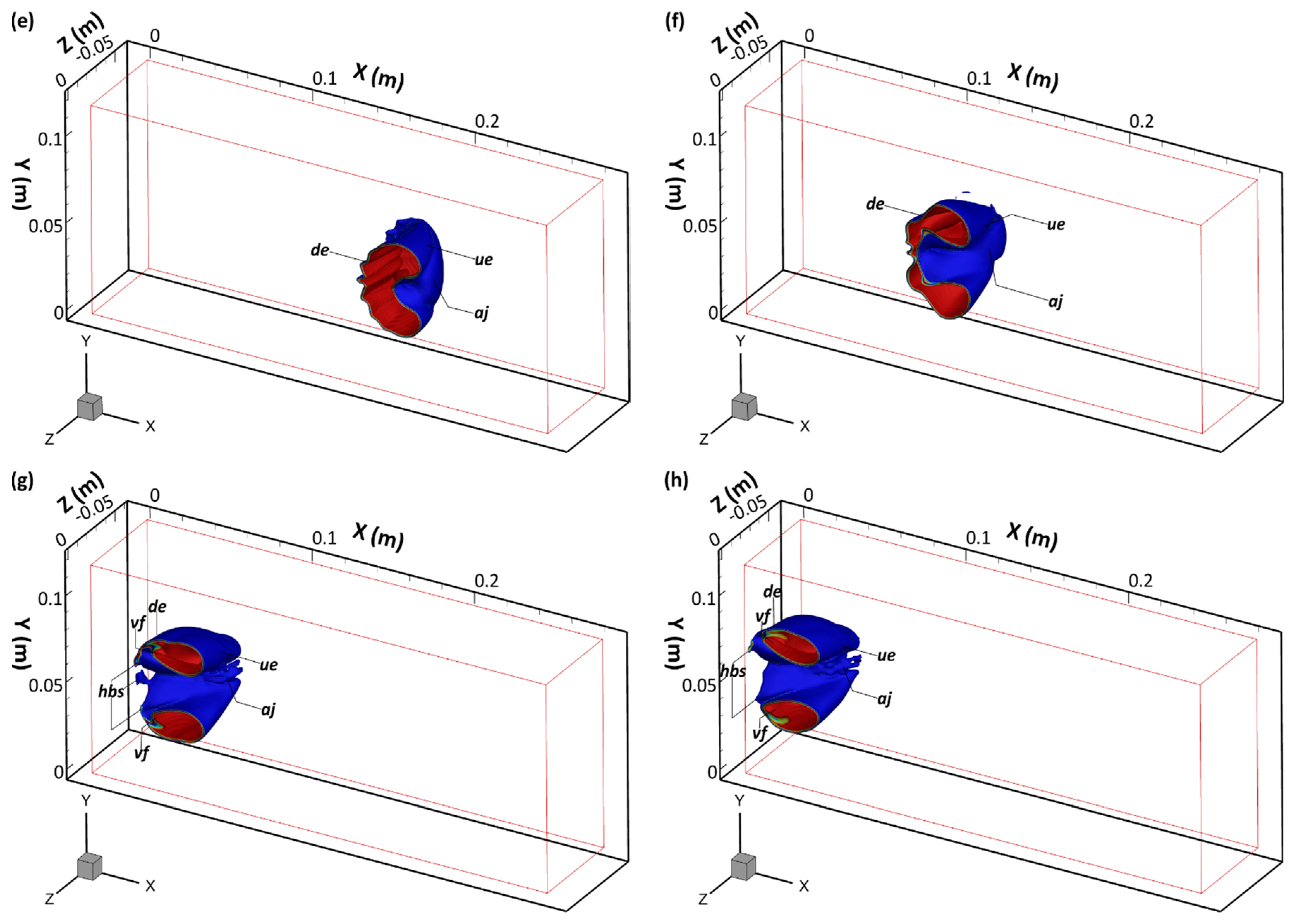
3.6. Shock–Bubble Interaction Process in 3D

Figure 10 shows eight snapshots of the predicted pressure iso-surfaces, revealing more clearly specific characteristics of the full bubble compression process and shock travel, particularly with respect to the observation of various wave patterns, wave propagation, bubble deformation, and the air-jet formation/development as a result of vorticity, which also leads to the formation of a pair of vortex filaments at the later phase of the SBI process.

Once the planar incident wave ($iw$) impacts the bubble’s upstream edge, a refracted wave ($rs$) is generated inside the bubble, and the $rs$ travels faster than the $iw$ because the speed of sound in the bubble gas, i.e., helium, is greater than the speed of sound in the surrounding gas, i.e., air. As shown in Figure 10a, at $t$ = 0.51, the $rs$ is already located closer towards the downstream bubble interface than the $iw$. As the upstream interface continues to deform and compress at $t$ = 0.68, the transmitted shock ($ts$) has emerged from the downstream end and has travelled a small distance away from the downstream interface, as shown in Figure 10b. It can also be seen from Figure 10b that the $iw$ has travelled about half of the bubble length and lags the $ts$. Figure 10c, at $t$ = 0.85, shows that the $ts$ has propagated more distance away from the downstream interface, with the $iw$ still trailing, but has itself travelled more than half of the length of the bubble. At $t$ = 1.02, the $iw$ has almost travelled the entire bubble length, and the bubble is also nearly entirely flattened at the upstream interface, as shown in Figure 10d. This is because the shocked bubble has been perturbed by continuous wave accelerations, thus subjecting it to considerable compression and distortion. At $t$ = 2.11, the $iw$ propagates across the bubble; vorticity production and deposition/distribution across the air–helium interface produced by the baroclinic effect during shock impingement on the upstream end of the bubble and the subsequent shock propagation across the bubble ensure that the associated rotational motion pulls a jet of ambient air ($aj$) through the centre of the bubble, as shown in Figure 10e. In addition, it is clearly observable from Figure 10e that at $t$ = 2.11, the bubble has been deformed considerably and is now ‘kidney-shaped’. At $t$ = 3.88, the $aj$ is more clearly visible from Figure 10f, as vorticity has intensified significantly. At the later phase of the shock–bubble interaction process ($t$ = 5.74 and $t$ = 8.44), the $aj$ has penetrated through the centre of the bubble and impinged on the downstream bubble end, with vorticity rolling up and dragging helium into a pair of vortex filaments ($vf$) at the downstream side of the deformed bubble. The $aj$ that pierces through the helium bubble volume and impinges on the downstream edge is analogous to the so-called RMI spike at a perturbed air–helium interface. It is worth pointing out that the present study elucidates how the $aj$ forms and develops, which has not been clearly detailed in the past literature, particularly with respect to a shock–cylindrical bubble interaction.

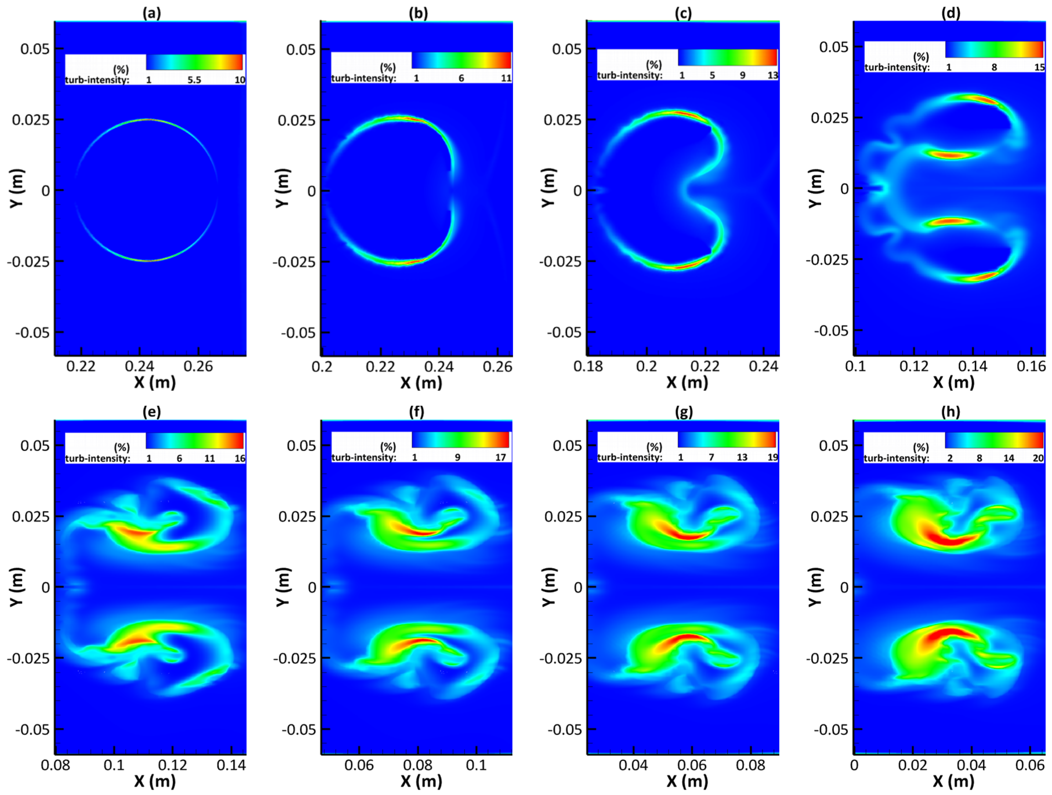
3.7. Turbulence Generation and Development

It has been shown above that the shock–bubble interaction process entails a wide range of complicated characteristics, from shock wave refraction and reflection, generation, and transport of vorticity, to the air-jet ($aj$) penetrating through the severely distorted bubble and the formation of vortex filaments. Nevertheless, to our best knowledge, there are rarely any previous experimental and numerical studies that have addressed one very important aspect of the shock–cylindrical bubble interaction process—turbulence generation and development. Figure 11 shows the predicted contours of turbulence intensity on the central x-y plane. As shown in Figure 11a, that turbulence starts to be generated initially in a small region at the bubble interface at the early stage ($t$ = 0.51). As time progresses, the bubble interface is deformed, as shown in Figure 11b,c at $t$ = 1.02 and $t$ = 2.11, and the upstream edge has caved in through the middle under the influence and penetration of the $aj$, but turbulence is still concentrated in a narrow region around the bubble interface, with the maximum turbulence intensity reaching about 11% at $t$ = 3.88, as shown in Figure 11d. Turbulence intensity gradually increases as the $aj$ continues to interact with the compressed upstream air–helium interface, promoting the generation and development of turbulence. Afterwards, the turbulence region starts to expand as the $aj$ has pierced the bubble and a pair of vortex filaments ($vf$) has formed, leading to an increase of the maximum turbulence level to about 14% around the $vf$ pair regions, as shown in Figure 11e at $t$ = 4.56. These vortical filaments are transported downstream, leading to an increased region of high turbulence intensity. Subsequently, it can be seen from Figure 11f–h that the turbulence region continues to expand gradually, with the turbulence level increasing steadily up to the maximum turbulence intensity around 20%, as shown in Figure 11h at $t$ = 8.44. Figure 11e–h also show that the highest turbulence intensity areas are within the $vf$.

4. Conclusions

The complex process of a cylindrical bubble interaction with a planar shock wave (Ma = 1.22) has been thoroughly investigated via a numerical study. The URANS computational approach is employed with a level set coupled with VOF method to capture the helium bubble and air interface accurately. An excellent agreement between the predicted velocities of the incident wave, refracted wave, transmitted wave, upstream interface, downstream interface, jet, vortex filament and the corresponding measured values is obtained. Furthermore, the predicted temporal variations of the interfacial characteristic scales, i.e., the length and width of the evolving interface, agree very well with the measured values too.

The developed simulations have been able to capture the main flow features, and the simulated 3D flow has helped to advance our current understanding of the complex process of shock–cylindrical bubble interaction, clearly illustrating the early phase of deformation and compression of the upstream edge of the helium-filled cylinder, followed by the air-jet formation that evolves and encroaches the downstream bubble end. In particular, the present study elucidates the mechanism on the air-jet formation and its development. Moreover, the complicated wave evolution, i.e., incident, transmitted wave, refracted wave, internally reflected wave, etc., is also clearly shown.

To our best knowledge, turbulence generation and development has not been presented/discussed in any of the previous relevant studies. The current study clearly reveals that turbulence is generated at the early phase of the shock–cylindrical bubble interaction process in the bubble upstream interface region, well before the formation of vortex filaments and even before the air-jet is formed. After a pair of distinctive vortex filaments is formed, turbulence is mainly generated around the vortex filament regions, with the maximum turbulence intensity reaching around 20%.

It is evident that the numerical approach used in the present study is robust and accurate, and there is a great potential for this numerical approach to be applied to study all kinds of shock–bubble interactions or even more general two-phase flows, where there is a need to capture interfaces accurately.

References

1. Niederhaus, J.H.J.; Greenough, J.A.; Oakley, J.G.; Ranjan, D.; Anderson, M.H.; Bonazza, R. A computational parameter study for the three-dimensional shock-bubble interaction. J. Fluid Mech. 2008, 594, 85–124. [Google Scholar] [CrossRef]
2. Layes, G.; Jourdan, G.; Houas, L. Distortion of a spherical gaseous interface accelerated by a plane shock wave. Phys. Rev. Lett. 2003, 91, 174502. [Google Scholar] [CrossRef] [PubMed]
3. Layes, G.; Jourdan, G.; Houas, L. Experimental investigation of the shock wave interaction with a spherical gas inhomogeneity. Phys. Fluids 2005, 17, 028103. [Google Scholar] [CrossRef]
4. Layes, G.; Le Metayer, O. Quantitative numerical and experimental studies of the shock accelerated heterogenous bubbles motion. Phys. Fluids 2007, 19, 042105. [Google Scholar] [CrossRef]
5. Zabusky, N.J.; Zeng, S.M. Shock cavity implosion morphologies and vortical projectile generation in axisymmetric shock-spherical fast/slow bubble interactions. J. Fluid Mech. 1998, 362, 327–346. [Google Scholar] [CrossRef]
6. Haas, J.F.L.; Sturtevant, B. Interaction of weak shock waves with cylindrical and spherical inhomogeneities. J. Fluid Mech. 1987, 181, 41–76. [Google Scholar] [CrossRef]
7. Jacobs, J.W. Shock-induced mixing of a light-gas cylinder. J. Fluid Mech. 1992, 234, 629–649. [Google Scholar] [CrossRef]
8. Jacobs, J.W. The dynamics of shock accelerated light and heavy gas cylinders. Phys. Fluids 1993, A5, 2239–2247. [Google Scholar] [CrossRef]
9. Marquina, A.; Mulet, P. A flux-split algorithm applied to conservative models for multicomponent compressible flows. J. Comput. Phys. 2003, 185, 120–138. [Google Scholar] [CrossRef]
10. Henderson, L.F. On the refraction of shock waves. J. Fluid Mech. 1989, 198, 365–386. [Google Scholar] [CrossRef]
11. Henderson, L.F.; Colella, P.; Puckett, E.G. On the refraction of shock waves at a slow-fast gas interface. J. Fluid Mech. 1991, 224, 1–27. [Google Scholar] [CrossRef]
12. Rudinger, G.; Somers, L.M. Behavior of small regions of different gases carried in accelerated gas flows. J. Fluid Mech. 1960, 7, 161–176. [Google Scholar] [CrossRef]
13. Ding, J.; Si, T.; Chen, M.; Zhai, Z.; Lu, X.; Luo, X. On the interaction of a planar shock with a three-dimensional light gas cylinder. J. Fluid Mech. 2017, 828, 289–317. [Google Scholar] [CrossRef]
14. Picone, J.M.; Boris, J.P. Vorticity generation by shock propagation through bubbles in a gas. J. Fluid Mech. 1988, 189, 23–51. [Google Scholar] [CrossRef]
15. Quirk, J.J.; Karni, S. On the dynamics of a shock–bubble interaction. J. Fluid Mech. 1996, 318, 129–163. [Google Scholar] [CrossRef]
16. Bagabir, A.; Drikakis, D. Mach number effects on shock-bubble interaction. Shock Waves 2001, 11, 209–218. [Google Scholar] [CrossRef]
17. Taniguchi, N.; Furuhata, R.; Sou, A.; Abe, A. Numerical simulation of shock wave bubble interaction for ballast water treatment. In Proceedings of the 3rd International Symposium of Maritime Sciences, Kobe, Japan, 10–14 November 2014. [Google Scholar]
18. Hayashi, K.; Sou, A.; Tomiyama, A. A volume tracking method based on non-uniform subcells and continuum surface force model using a local level set function. Comput. Fluid. Dyn. J. 2006, 15, 95–101. [Google Scholar]
19. Yee, H.C.; Warming, R.F.; Harten, A. Implicit total variation diminishing (TVD) schemes for steady-state calculations. J. Comput. Phys. 1985, 57, 327–360. [Google Scholar] [CrossRef]
20. Wang, Z.; Yu, B.; Chen, H.; Zhang, B.; Liu, H. Scaling vortex breakdown mechanism based on viscous effect in shock cylindrical bubble interaction. Phys. Fluids 2018, 30, 126103. [Google Scholar] [CrossRef]
21. Chen, J.; Qu, F.; Wu, X.; Wang, Z.; Bai, J. Numerical study of interactions between shock waves and a circular or elliptic bubble in air medium. Phys. Fluids 2021, 33, 043301. [Google Scholar] [CrossRef]
22. Singh, S.; Battiano, M.; Myong, R.S. Impact of bulk viscosity on flow morphology of shock accelerated cylindrical light bubble in diatomic and polyatomic gases. Phys. Fluids 2021, 33, 066103. [Google Scholar] [CrossRef]
23. Onwuegbu, S.; Yang, Z. Numerical analysis of shock interaction with a spherical bubble. AIP Adv. 2022, 12, 025215. [Google Scholar] [CrossRef]
24. Shyue, K.M. An efficient shock-capturing algorithm for compressible multicomponent problems. J. Comput. Phys. 1998, 142, 208–242. [Google Scholar] [CrossRef]
25. Serthian, J.A.; Smereka, P. Level set methods for fluid interfaces. Ann. Rev. Fluid Mech. 2003, 35, 341–372. [Google Scholar] [CrossRef]
26. Olsson, E.; Kreiss, G.; Zahedi, S. A Conservative Level Set Method for Two Phase Flow II. J. Comput. Phys. 2007, 225, 785–807. [Google Scholar] [CrossRef]
27. Van Leer, B. Toward the Ultimate Conservative Difference Scheme. V. A Second Order Sequel to Godunov’s Method. J. Comput. Phys. 1979, 32, 101–136. [Google Scholar] [CrossRef]
28. Holleman, R.; Fringer, O.; Stacey, M. Numerical diffusion for flow-aligned unstructured grids with application to estuarine modelling. Int. J. Numer. Methods Fluids 2013, 72, 1117–1145. [Google Scholar] [CrossRef]
29. Zubair, M.; Abdullah, M.Z.; Ahmad, K.A. Hybrid mesh for nasal airflow studies. Comput. Math. Methods Med. 2013, 2013, 727362. [Google Scholar] [CrossRef] [PubMed]
30. Ingram, D.M.; Causon, D.M.; Mingham, C.G. Developments in Cartesian cut cell methods, Math. Comput. Simul. 2013, 61, 561–572. [Google Scholar] [CrossRef]
31. Johnson, M.W. A novel Cartesian CFD cut cell approach. Comput. Fluids 2013, 79, 105–119. [Google Scholar] [CrossRef]
32. Taylor, G.I. Formation of a vortex ring by giving an impulse to a circular disk and then dissolving it away. J. Appl. Phys. 1953, 24, 104–105. [Google Scholar] [CrossRef]
Figure 1. Computational domain plus the initial and boundary conditions.
Modelling 05 00026 g001
Figure 2. (a) Computational mesh; and (b) close view of fine mesh around bubble from adaptive mesh refinement (AMR).
Modelling 05 00026 g002
Figure 3. Predictions obtained using three meshes for the mesh independence study.
Modelling 05 00026 g003
Figure 4. Comparison between the predictions obtained from inviscid simulations, different turbulent models, and the experimental data.
Modelling 05 00026 g004
Figure 5. Comparison between the predicted dimensionless displacements of the upstream edge against the experimental data [6] and the previous numerical results [21].
Modelling 05 00026 g005
Figure 6. Comparison between the predicted dimensionless displacements of the downstream edge against the experimental data [6] and the previous numerical results [20].
Modelling 05 00026 g006
Figure 7. Comparison between the predicted and measured bubble evolution.
Modelling 05 00026 g007
Figure 8. Snapshots of experimental shadow-photographs (left) and simulated images (right) on the central x-y plane at: (a) t = 0.34; (b) t = 0.51; (c) t = 0.6; (d) t = 0.85; (e) t = 2.11; (f) t = 3.88; (g) t = 5.74; and (h) t = 8.44.
Modelling 05 00026 g008
Figure 9. Snapshots of vorticity contours on the central x-y plane at: (a) t = 0.51; (b) t = 0.68; (c) t = 1.02; (d) t = 2.11; (e) t = 3.88; (f) t = 5.74; (g) t = 6.92; and (h) t = 8.44.
Modelling 05 00026 g009
Figure 10. Pressure iso-surfaces at: (a) t = 0.51; (b) t = 0.68; (c) t = 0.85; (d) t = 1.02; (e) t = 2.11; (f) t = 3.88; (g) t = 5.74; and (h) t = 8.44.
Modelling 05 00026 g010aModelling 05 00026 g010b
Figure 11. Contours of turbulent intensity along the x-y plane at: (a) t = 0.51; (b) t = 1.02; (c) t = 2.11; (d) t = 3.88; (e) t = 4.56; (f) t = 5.74; (g) t = 6.92; and (h) t = 8.44.
Modelling 05 00026 g011