Article

Integrated Modeling of Coastal Processes Driven by an Advanced Mild Slope Wave Model

by
Michalis K. Chondros
1,2,*,
Anastasios S. Metallinos
1,2 and
Andreas G. Papadimitriou
1,2
1
Laboratory of Harbour Works, School of Civil Engineering, National Technical University of Athens, 5 Heroon Polytechniou Str., 15780 Zografou, Greece
2
Scientia Maris, Agias Paraskevis Str. 117, 15234 Chalandri, Greece
*
Author to whom correspondence should be addressed.
Modelling 2024, 5(2), 458-482; https://doi.org/10.3390/modelling5020025
Submission received: 30 January 2024 / Revised: 4 April 2024 / Accepted: 5 April 2024 / Published: 11 April 2024

Abstract

:
Numerical modeling of wave transformation, hydrodynamics, and morphodynamics in coastal regions holds paramount significance for combating coastal erosion by evaluating and optimizing various coastal protection structures. This study aims to present an integration of numerical models to accurately simulate the coastal processes with the presence of coastal and harbor structures. Specifically, integrated modeling employs an advanced mild slope model as the main driver, which is capable of describing all the wave transformation phenomena, including wave reflection. This model provides radiation stresses as inputs to a hydrodynamic model based on Reynolds-averaged Navier–Stokes equations to simulate nearshore currents. Ultimately, these models feed an additional model that can simulate longshore sediment transport and bed level changes. The models are validated against experimental measurements, including energy dissipation due to bottom friction and wave breaking; combined refraction, diffraction, and breaking over a submerged shoal; wave transformation and wave-generated currents over submerged breakwaters; and wave, currents, and sediment transport fields over a varying bathymetry. The models exhibit satisfactory performance in simulating all considered cases, establishing them as efficient and reliable integrated tools for engineering applications in real coastal areas. Moreover, leveraging the validated models, a numerical investigation is undertaken to assess the effects of wave reflection on a seawall on coastal processes for two ideal beach configurations—one with a steeper slope of 1:10 and another with a milder slope of 1:50. The numerical investigation reveals that the presence of reflected waves, particularly in milder bed slopes, significantly influences sediment transport, emphasizing the importance of employing a wave model that takes into account wave reflection as the primary driver for integrated modeling of coastal processes.

1. Introduction

The prediction of coastal morphodynamics at a time span of years to decades [1,2,3,4,5,6], induced by the combined effect of waves and currents, has been at the forefront of coastal engineering research for several decades, with the ultimate goal to thoroughly investigate the complex nearshore processes and mitigate erosion. To combat the adverse effects of erosion, coastal protection works (e.g., breakwaters, groins, and seawalls) have been constructed by engineers focusing predominantly on reducing the incident wave energy. In order to optimize the layout and configuration of coastal protection schemes, numerical models [7,8,9,10,11,12,13,14] are of paramount importance to simulate the coastal processes taking place in a coastal area. Although several numerical models are available nowadays, researchers and the engineering community still to this day develop and utilize numerical models, with the aim to simulate even more coastal processes and minimize the required computational resources. Despite the numerous options available, each numerical model is associated with specific advantages and limitations as far as resolving the dominant coastal processes is concerned [15].
When dealing with wave propagation in the presence of shore parallel protection structures, such as seawalls and detached breakwaters, the processes of wave diffraction and reflection become dominant in driving wave transformation, hydrodynamics, and sediment transport. Even though wave diffraction and how it affects coastal hydrodynamics and morphodynamics has been studied rigorously, both experimentally [16,17,18,19,20,21,22] and numerically [15,23,24,25,26,27,28,29], the effect of wave reflection on longshore hydrodynamics and sediment transport remains an ambiguous topic for researchers up until this day [30]. A comprehensive review of the effect of seawalls on the beach [31] concluded that due to the absence of field data, it is unclear whether the longshore sediment transport rates along the seawall increase [32,33,34] or decrease [35,36]. This is further exemplified by the conflicting reports on the effect of longshore currents and sediment transport reported in the experimental study of [37,38] on one hand, and the field study of [39] on the other. Therefore, to what extent wave reflection affects the longshore coastal processes is still not universally agreed upon by the engineering community [30,40].
To resolve the abovementioned processes of wave diffraction and reflection, wave models based on the so-called phase-resolving [41] approach have been utilized to describe the temporal and spatial resolution of the wave regime to account for the phase difference of the wave trains. The most notable representatives of this category of wave models are Boussinesq-type wave models (e.g., [42,43,44,45]) and mild slope wave models [46,47,48,49].
Presently, Boussinesq-type models coupled with sediment transport modules are encountered in the literature of coastal engineering [50,51,52,53] for several applications, ranging from coastal morphodynamics in the vicinity of emerged coastal protection structures [51,54] or even submerged breakwaters [15,54]. Despite their good performance and the significant steps taken to maximize their computational efficiency, Boussinesq-type models are seldom applied in practical coastal engineering applications (i.e., coastal areas of up to 5 km × 5 km) due to their increased nonlinearity, resulting in rather strict numerical stability restrictions and thus longer simulation times.
Mild slope wave models (e.g., [46,49,55,56]) present an attractive alternative to Boussinesq-type wave models for applications of wave disturbance inside ports, but their application in coastal engineering is more limited [13,57]. Karambas and Samaras [13] developed a linear time-dependent mild slope derived from the hyperbolic approximation to the mild slope equation and used it as a wave driver to simulate wave-generated currents and morphology for various configurations of emerged coastal protection structures. Still, the looser stability restrictions of the mild slope wave equation compared to the Boussinesq-type wave models renders them particularly enticing as the main wave driver for the prediction of wave-generated currents and subsequent sediment transport rates.
The scope of this paper is to present the validation and application of the integration of models, consisting of an irregular and nonlinear mild slope wave model [49,58] coupled with a hydrodynamic [59] and sediment transport model [5], to thoroughly investigate wave transformation, wave-generated hydrodynamics, and sediment transport in coastal regions, with or without coastal works. Of particular importance is the validation of the energy dissipation mechanism for the wave model, constituting the main driver of nearshore processes, as well as a parametric numerical application to assess the effect of wave reflection due to a seawall in longshore hydrodynamics and sediment transport.

2. Mathematical Background of the Implemented Models

The equations that govern the wave, hydrodynamic, and sediment transport models, as well as the main processes they are capable of resolving, are presented in the present section.

2.1. The Hyperbolic Mild Slope Wave Propagation Model (HMS)

The foundation of the wave model relies on solving the hyperbolic version of the mild slope wave equation, describing the spatial and temporal evolution of the free sea surface elevation and the water particle velocities. It is capable of simulating the generation and propagation of regular and irregular waves. It is noted that the background and features of the numerical model have been presented in the recent publication of [58]; therefore, for the sake of brevity, only the governing equations and energy dissipation terms will be presented below. Based on [48,49], the continuity and momentum equations for linear harmonic wave propagation in coastal waters of mild sloping beds accounting for energy dissipation terms are as follows:
ζ t + · ( U h ) = w b ζ t
( U h ) t + c 2 n ( n ζ ) = v h 2 · U w b f U
where ζ represents the elevation of the sea surface, h denotes the water depth, U = ( U ,   V ) represents the vector of mean water particle velocity, with U and V being the mean velocities in the horizontal dimensions (x and y), respectively, c is the phase celerity, n = ( 1 / 2 + k h / sinh k h ) , k is the wave number, v h is the horizontal eddy viscosity coefficient responsible for replicating partial wave reflection, w b f denotes energy dissipation due to bottom friction, and w b denotes energy dissipation due to depth-induced breaking.
Energy dissipation w b f = E f / E ( E = ρ g H r m s 2 / 8 , with H r m s being the root mean square wave height, ρ the sea water density and g the acceleration of gravity) due to bottom friction is given by ([60]):
E f = 1 6 π c f w / 2 g ( ω H sinh k h ) 3 for regular waves and E f = 1 8 π c f w / 2 g ( ω H r m s sinh k h ) 3 for irregular waves
where c f w is a wave friction coefficient [61], g is the acceleration of gravity, and ω is the angular frequency.
Energy dissipation w b = E b / E due to depth-induced breaking is calculated as shown in the following [61]:
E b = a 4 Q b f p ρ g H m a x 2
where a is a calibration coefficient, f p is wave frequency at spectral peak, Q b is the fraction of breaking waves, obtained by solving the following relationship 1 Q b ln Q b = ( H r m s H m a x ) 2 , assuming a Rayleigh distribution of the wave heights, and H m a x is the maximum wave height based on a Miche-type breaking the criterion [62] as follows:
H m a x = γ 1 k tan h ( k γ 2 h γ 1 )
where γ 1 and γ 2 are constants with typical values of 1.0 and 0.8, respectively.
It is noted that the model can simulate irregular wave propagation and transformation given that the incident wave energy spectrum should be discretized into frequency and direction components. Each discrete component, representing a regular wave, is then solved independently. Upon the independent solution of each component, at each time step, a synthesis of the free surface is performed through linear superposition to yield the irregular sea state in the entire numerical domain and compute the desired magnitudes, H r m s and H s , as detailed in [58].

2.2. The Hydrodynamic Model (HYD)

The model, which simulates the hydrodynamic field and is henceforth denoted as the HYD, takes into account various influencing factors. It is capable of simulating nearshore currents generated by waves, wind, and tides. The model solves the depth-integrated incompressible Reynolds-averaged Navier–Stokes equations, composed of the following continuity and momentum equations [5]:
η ¯ t + ( U h ) x + ( V h ) y = P
U t + U U x V U y + g η ¯ x = 1 ρ h ( S x x x + S x y y ) + 1 h x ( ν h h U x ) + 1 h y ( ν h h U y ) + f V + τ s x ρ h τ b x ρ h + P x
V t + U V x V V y + g η ¯ y = 1 ρ h ( S y y y + S x y x ) + 1 h x ( ν h h V x ) + 1 h y ( ν h h V y ) f U + τ s y ρ h τ b y ρ h + P y
where η ¯ denotes the mean sea surface elevation, U and V denote the depth-averaged current velocities in the two horizontal directions ( x and y ), respectively, ρ is the seawater density, h is the total water depth, f is the Coriolis coefficient, g is the gravitational acceleration, v h is the horizontal turbulent eddy viscosity coefficient, τ s x and τ s y are the x- and y-components of the wind shear stress at the air–sea interface, τ b x and τ b y , are x- and y-components of the bottom friction shear stresses, and P, Px, Py are external discharges either added or subtracted for an external point source or sink, respectively. The simulation of wave-generated currents involves the incorporation of the radiation stress components S x x ,   S x y , and S y y .
The calculations are executed on a staggered Arakawa C-type grid, wherein the velocity components are computed between neighboring sea-level grid cells. The temporal resolution of the governing equations can be achieved using an explicit Euler or 3rd Order Strong Stability Preserving Runge–Kutta scheme. In the spatial domain, a 1st Order Central Space finite difference scheme is employed.

2.3. The Sediment Transport and Sedimentation/Erosion Model (SDT)

The SDT model is a 2D non-cohesive sediment transport model designed to calculate sediment transport rates and predict the coastal bed evolution. It considers the combined impact of waves and currents on sediment dynamics. In this study, sediment transport rates were determined using the total load sediment transport formula proposed by Soulsby and van Rijn [63]. This formula incorporates individual contributions from bedload and suspended load transport, as well as the bedload-only formula by Soulsby [63]. For brevity reasons, only the basic equations of the formula of Soulsby and van Rijn, hereafter denoted as SvR, will be presented.
The critical current velocity, constituting the threshold of initiation of sediment motion, is calculated by the following relationship [63,64]:
U c r { 0.19 ( d 50 ) 0.1 l o g 10 ( 4 h d 90 ) ,             when   0.05 d 50 < 0.5   mm 8.5 ( d 50 ) 0.6 l o g 10 ( 4 h d 90 ) ,             when   0.5 d 50 2.0   mm
where d 50 is the median sediment diameter and d 90 denotes the diameter where ninety percent of the distribution has a smaller particle size.
The sediment transport rate resulting from bedload is computed using the following equation under the combined influence of waves and currents [63]:
q b = A b ( U ¯ t o t 2 + 0.018 C D U r m s 2 U c r ) U ¯ t o t
where U ¯ t o t = U ¯ 2 + V ¯ 2 is the depth-averaged current velocity, U r m s is the root-mean-square wave orbital velocity amplitude near the bed, A b a bedload multiplication factor, and C D is the drag coefficient due to currents only.
The bedload multiplication factor A b is given by [63] the following:
A b = 0.005   h   ( d 50 h ( Δ g d 50 ) )
where Δ = ρ s / ρ is the relative sediment density and g is the acceleration of gravity.
The drag coefficient C D is calculated by the following relationship [63]:
C D = ( κ ln ( h z 0 ) 1 ) 2
where κ is the von Karman constant and z 0 is the bed roughness length.
Subsequently, the suspended sediment transport rate is computed as follows [63]:
q s = A s ( U ¯ t o t 2 + 0.018 C D U r m s 2 U c r ) U ¯ t o t
where A s is the suspended load multiplication factor calculated by the following equation:
A s = 0.012   d 50 D * 0.6 ( Δ g d 50 ) 1.2
where D * = [ g ( s 1 ) ν 2 ] 1 / 3 is the dimensionless grain size.
The equation solved by the model to calculate the change in bed elevation, z b , over time is the well-known sediment mass balance equation or the Exner equation as follows:
( 1 n p ) z b t + · q t = 0
where n p is the sediment porosity and q t = q b + q s the total sediment transport rate.
The calculations are executed on a regular grid, and the rates of bed level change are determined by discretizing the Exner equation using an Upwind, Lax–Wendroff, or Euler-WENO scheme [65] at each time step. The SDT model takes as input wave orbital velocities obtained by HMS and current speeds, as calculated by the hydrodynamic model HYD, to calculate the total load sediment transport and bed level change at each time step.

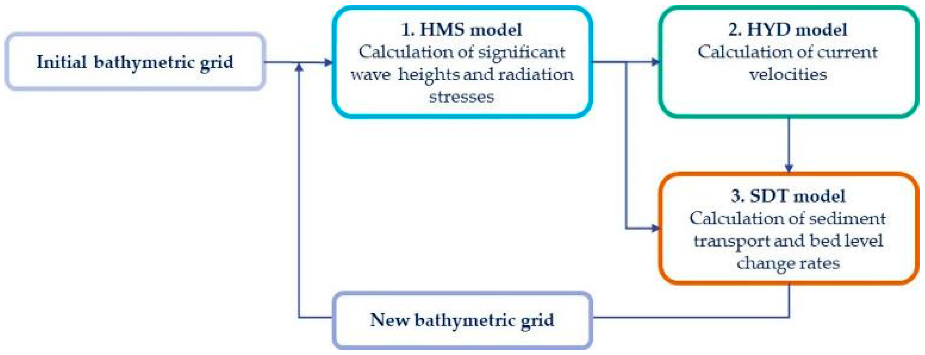
2.4. Implementation Sequence of Numerical Models

The models are linked in a “one-way” coupling manner and they are applied sequentially, with each model feeding the next. Initially, the wave model, HMS, is implemented to compute the spatial distribution of significant wave heights and radiation stresses across the entire numerical domain. Subsequently, the radiation stresses serve as inputs for the hydrodynamic model, HYD, which calculates current velocities. Following this, the wave and hydrodynamic results are provided as input data to the sediment transport model, SDT, to compute sediment transport and bed evolution rates. Finally, based on these rates, a new bathymetry is created, and a new cycle of simulations can be initiated. These procedural steps are outlined in the flowchart depicted in Figure 1.

3. Validation of Individual Numerical Models

The capability of the three distinct numerical models to simulate the dominant wave transformation processes and subsequent hydrodynamic fields and sediment transport in the nearshore area is thoroughly evaluated in the subsections below. Specific focus is given to the interaction of the models, their performance in complex bathymetries, and the wave–structure interaction capabilities.

3.1. Validation of the Mild Slope Wave Model (HMS)

In this section, we assess the effectiveness of the HMS wave model in replicating key wave transformation processes occurring in the nearshore region. Emphasis is placed on evaluating the energy dissipation mechanisms within the HMS model, as they play a crucial role in initiating the formation of longshore currents and sediment transport. For this reason, a comparison of model results with three benchmark experiments is carried out, with the first experiment concerning energy loss of regular waves due to bottom friction [66], the second one concerning wave breaking of irregular unidirectional waves on a plane-sloping beach [67], and the third one dealing with wave transformation and breaking of multidirectional waves over a submerged shoal [68].

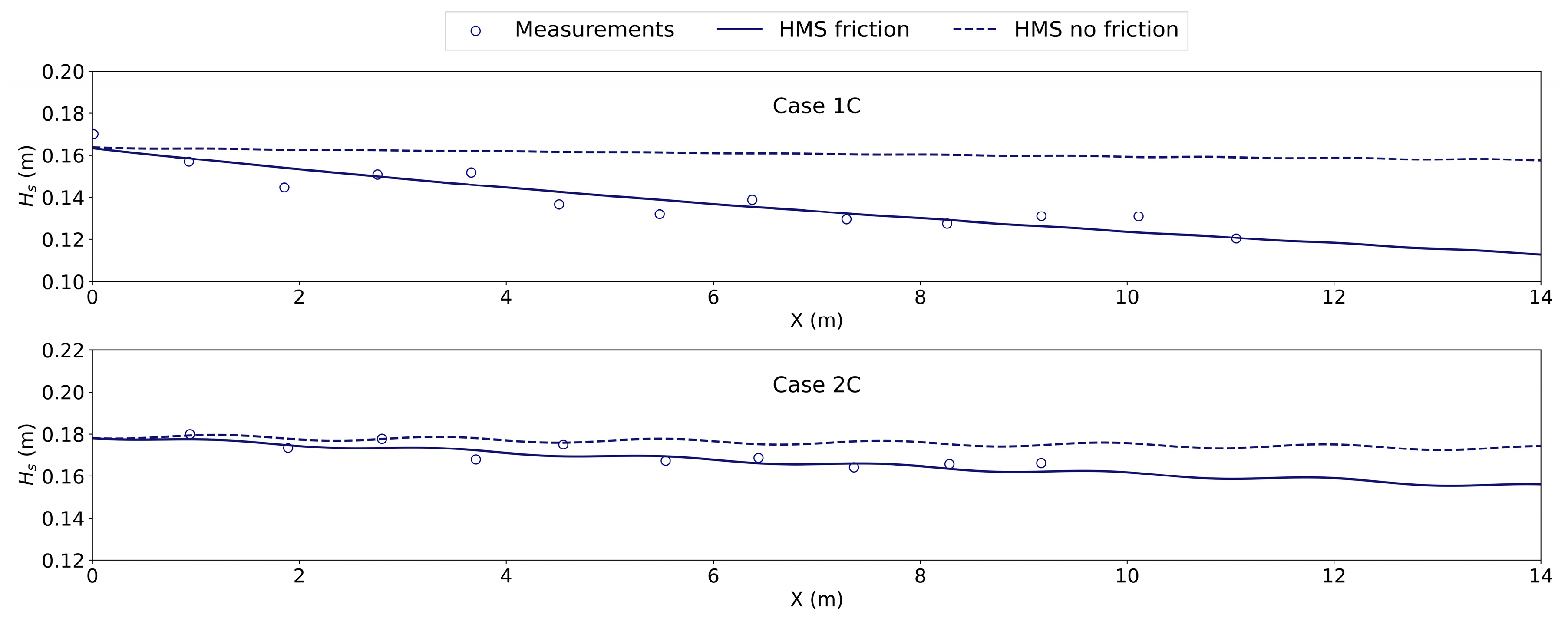
3.1.1. Energy Dissipation due to Bottom Friction on a Rippled Bed [66]

The first benchmark experiment on which the HMS results were validated concerns the decay of regular waves over a rippled sandy bed due to bottom friction. The experiments were carried out in a 21 m long and 61 cm wide wave channel in HR Wallingford, with a relatively straightforward layout comprised of a constant still water depth of 0.5 m. An 11 m long sand bed was placed in the central, horizontal portion of the channel, beginning about ten meters downwave from the wavemaker, with a median sediment grain size of d 50 = 2 mm. Above this sandy patch, all the measurements of the wave height and orbital velocity were undertaken. In total, six tests were conducted with varying incident wave characteristics, as well as the geometry of the rippled bed.
The numerical grid consists of 500 cells in the x-direction and 10 cells in the y-direction with an equal spatial step size of 0.05 m. Two test cases are reproduced with the HMS model corresponding to Case 1C and Case 2C as shown in [66]. The incident wave characteristics and the ripple parameters are compiled and shown in Table 1. It is noted that the wave friction factor is calculated internally by the numerical model, utilizing the formula of [69] and the method of [64] to specify the skin friction coefficient due to the rippled bedforms. Sponge layers are placed behind the wavemaker and at the eastern boundary to absorb the reflected wave energy. The duration of the model simulations is set at 100 s.
Figure 2 illustrates the wave heights over the sandy rippled bed for both cases as simulated with the HMS model considering bottom friction (HMS friction in the Figure 2 legend) superimposed with the experimental measurements and simulation results without considering the effect of bottom friction (HMS no friction in the Figure 2 legend).
Overall, the results of the model exhibit excellent agreement with the experiment, validating its capability to numerically reproduce the energy loss due to bottom friction for a case of more intense (Case 1C) or milder (Case 2C) wave decay.

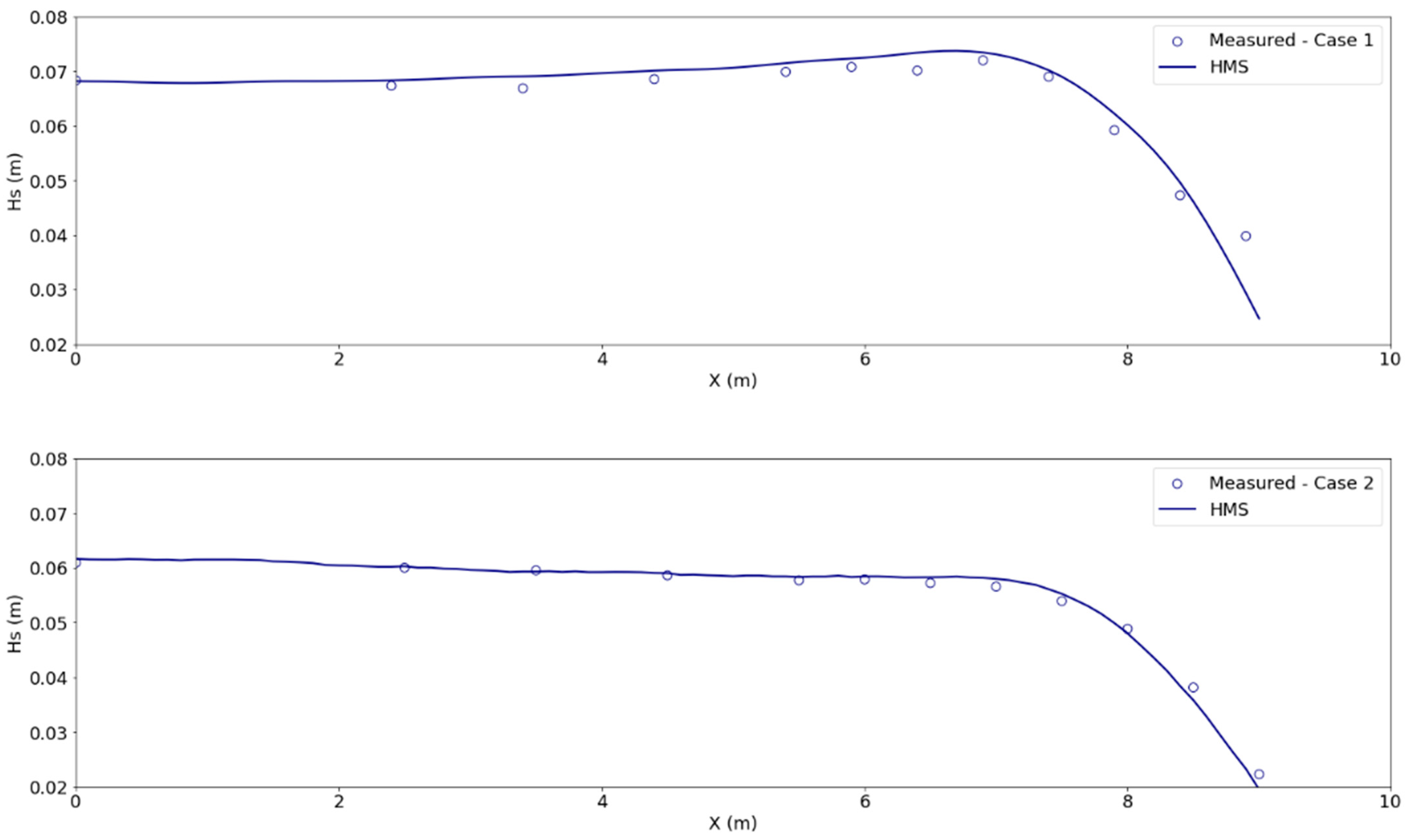
3.1.2. Wave Breaking of Irregular Unidirectional Waves over a Plane-Sloping Beach [67]

As an additional validation test, we considered the experiments conducted by [67] that focused on the breaking of irregular waves (Pierson–Moskowitz spectrum) on a beach with a constant 1:20 slope. Hereafter, two cases are reproduced with the HMS model: the first with a peak frequency f p = 0 . 6 (Case 1), corresponding to spilling breakers, and the second with a peak frequency f p = 1 . 0 (Case 2), corresponding to plunging breakers. Waves travel in an experimental flume with a constant depth equal to 0.47 m for 10 m, and then they propagate over the beach. The free surface was measured using 12 probes positioned along the sloping bed at locations corresponding to still water depths of 0.47 m, 0.35 m, 0.3 m, 0.25 m, 0.2 m, 0.175 m, 0.15 m, 0.125 m, 0.1 m, 0.075 m, 0.05 m, and 0.025 m.
The numerical grid has a uniform spatial step size, equal to 0.1 m, in both directions. To accommodate the placement of sponge layers, the numerical flume was extended by 20 m downwave from the wave generator. The incident wave energy spectrum is discretized using 25 frequencies. The calculated significant wave heights ( H s ) for both cases are presented in Figure 3 in comparison to the experiment of [67]. It is noted that in both cases, the γ 2   calibration parameter of the depth-induced energy dissipation was set at a value of 0.72 (instead of the default value of 0.8) to better capture the point of breaking initiation.
The analysis of Figure 3 reveals a high level of agreement for both simulated test cases between the HMS results and the experimental data. A slight overprediction of the wave heights as the waves shoal up until they reach the dissipation point is observed in Case 1, while the largest underprediction is located in the most landward gauge near the coastline since the model does not consider wave setup. For Case 2, there is a nearly perfect agreement observed between HMS results and experimental data. Overall, the capability of the model to accurately reproduce the wave energy dissipation rate due to bathymetry breaking for unidirectional irregular waves is verified.

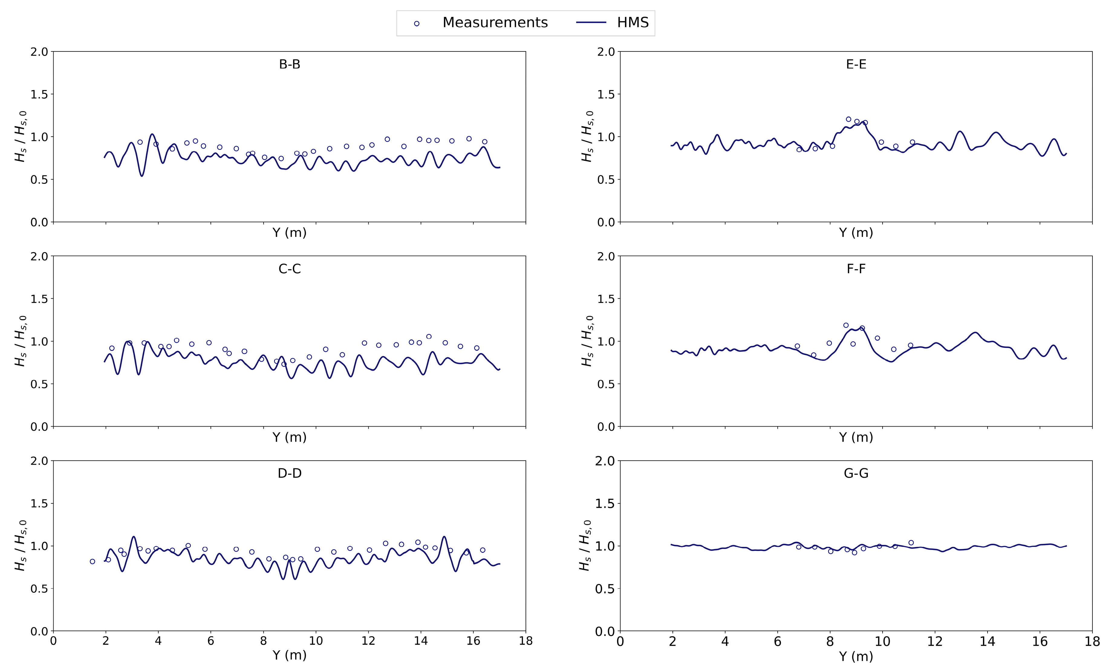
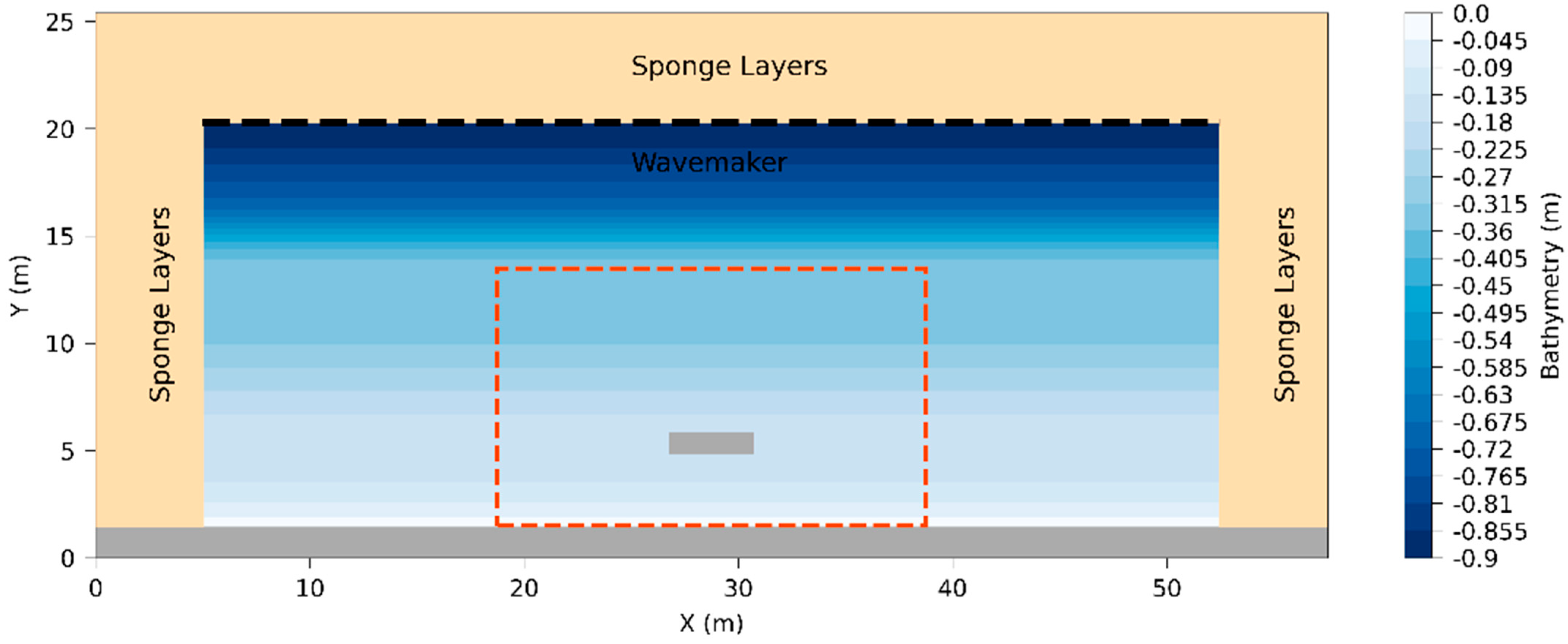
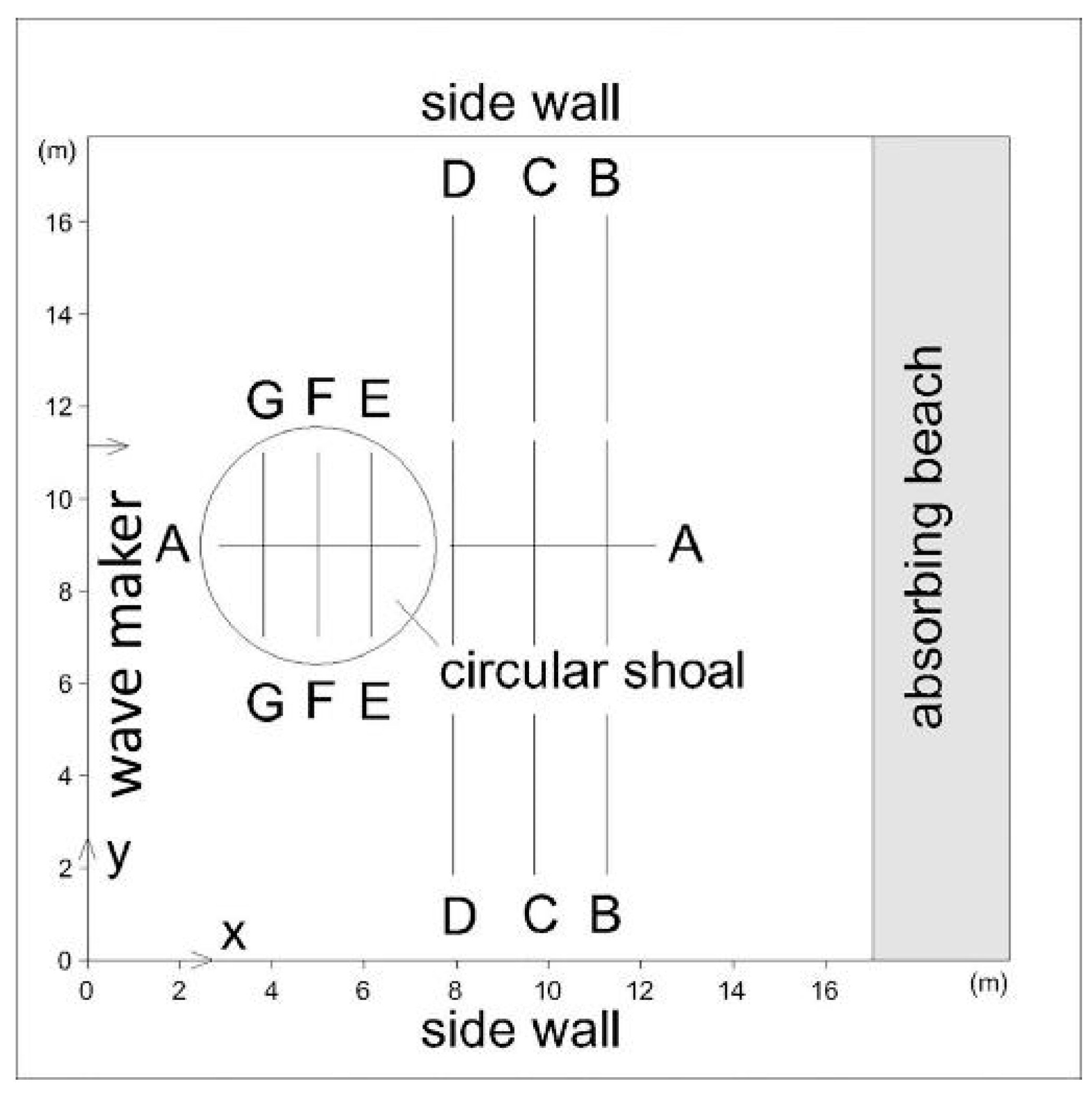
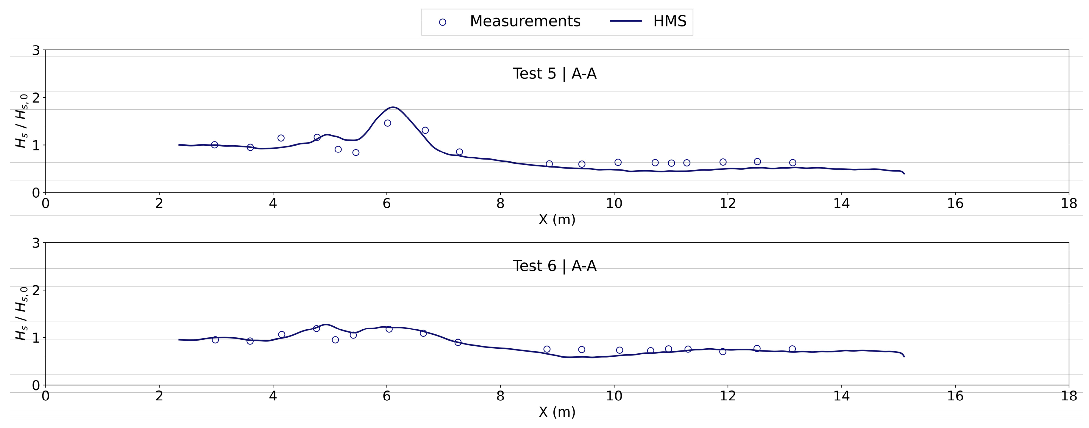
3.1.3. Wave Breaking of Irregular Multidirectional Waves over a Submerged Shoal [68]

To evaluate the performance of the wave model in predicting the wave energy dissipation due to bathymetric breaking in a more complex 2D case for irregular multidirectional waves, the experiments by [68] have been reproduced numerically. The authors in [68] conducted a series of physical experiments in the directional wave basin at the University of Delaware and thoroughly studies the wave transformation processes over a circular submerged shoal. The wave basin was 18 m long and 18.2 m wide, and the center of the circular slope was situated at x = 5 m and y = 8.98 m. The experimental layout along with the positions of the transects where wave heights were measured is shown in Figure 4. The wave characteristics were measured at a total of 126 points around the shoal, spread between one longitudinal transect (AA) over the shoal and six transversal transects (BB, CC, EE, FF, and GG) situated behind and on top of the shoal. To minimize wave reflection, the water depth outside the shoal was constant and equal to 0.4 m, while the water depth on top of the shoal was 0.03 m.
The performance of the present hyperbolic mild slope wave model for the transformation of non-breaking and breaking regular waves over the shoal has been validated and shown in the publication by [49]. In this research, two different test conditions were reproduced numerically, concerning the wave breaking and transformation of irregular multidirectional waves with a narrow (Test 5) and broad (Test 6) directional spreading. The particular cases will serve the purpose of thoroughly investigating the capability of the model to simulate irregular wave transformation under the combined effect of refraction, diffraction, and bathymetric breaking. Waves are generated using a TMA [70] spectrum source function, and the wave characteristics of the two simulated test cases are shown in Table 2, where θ ο is the incident direction in relation to north, γ is the spectrum peak enhancement factor, and σ is the directional spreading parameter.
The numerical grid is constructed with 800 and 1000 cells in the x- and y-directions, respectively. The spatial step size equals 0.025 m in both directions. Sponge layers, with a width of 20 cells, are placed at all the lateral boundaries to absorb the reflected wave energy. The simulation time is set to 80 s, and the last five periods are used to extract the numerical results of the significant wave height. Figure 5 shows the normalized wave height along the longitudinal transect AA for Test 5 and Test 6, respectively.
In general, the model predicts in a satisfying manner the wave energy dissipation due to waves breaking on top of the slope, with a minor overprediction of the breaking wave height for waves with a narrow directional spreading (Test 5). On the other hand, the wave height distribution along transect AA closely aligns with the experiment for the broad-banded multidirectional case (Test 6).
The simulated normalized wave heights for the transversal transects are compared to the experimental measurements and shown for both Test 5 and Test 6 in Figure 6 and Figure 7, respectively.
The model predicts the spatial distribution of the wave height and the focusing of the wave energy on top of the shoal (transects EE, FF, GG) for the narrow-banded case reasonably well. At the transects directly behind the shoal (BB, CC, DD), the wave heights are underpredicted, especially behind the center of the shoal. Since the model does not account for wave–wave interactions, this discrepancy is expected due to the highly nonlinear nature of the waves breaking and reforming behind the shoal, as has also been identified by [71].
For the directional case with a broad-banded spectrum, the focus of the wave energy as waves propagate on top of the shoal (transects EE, FF, GG) is reproduced in a very satisfying manner by the numerical model, with the wave heights being more “smoothed out”, as was expected compared to the narrow-banded case. In a manner akin to the previously mentioned case, a slight underprediction of the normalized wave heights can be identified at the center behind the shoal. It should be noted that some more abrupt variations at transects BB, CC, and DD, especially near the boundaries of the domain, are attributed in part to reflected waves for the lateral boundaries, which, despite the presence of the sponge layers, were present due to high deviation of wave incidence angles at the wavemaker (±45°) with respect to the mean direction of wave incidence.

3.2. Validation of the Hydrodynamic Model (HYD)

In this section, a thorough validation of the HYD hydrodynamic model is carried out. Within this research framework, the performance of the model in simulating wave-generated currents is evaluated. Hence, an experiment containing wave–structure interaction and the resulting hydrodynamics was considered as a best-case scenario. To this end, the well-known DELOS experiment [72], concerning wave transformation and hydrodynamics in the vicinity of low-crested structures, was selected to be reproduced numerically with the combination of HMS and HYD.

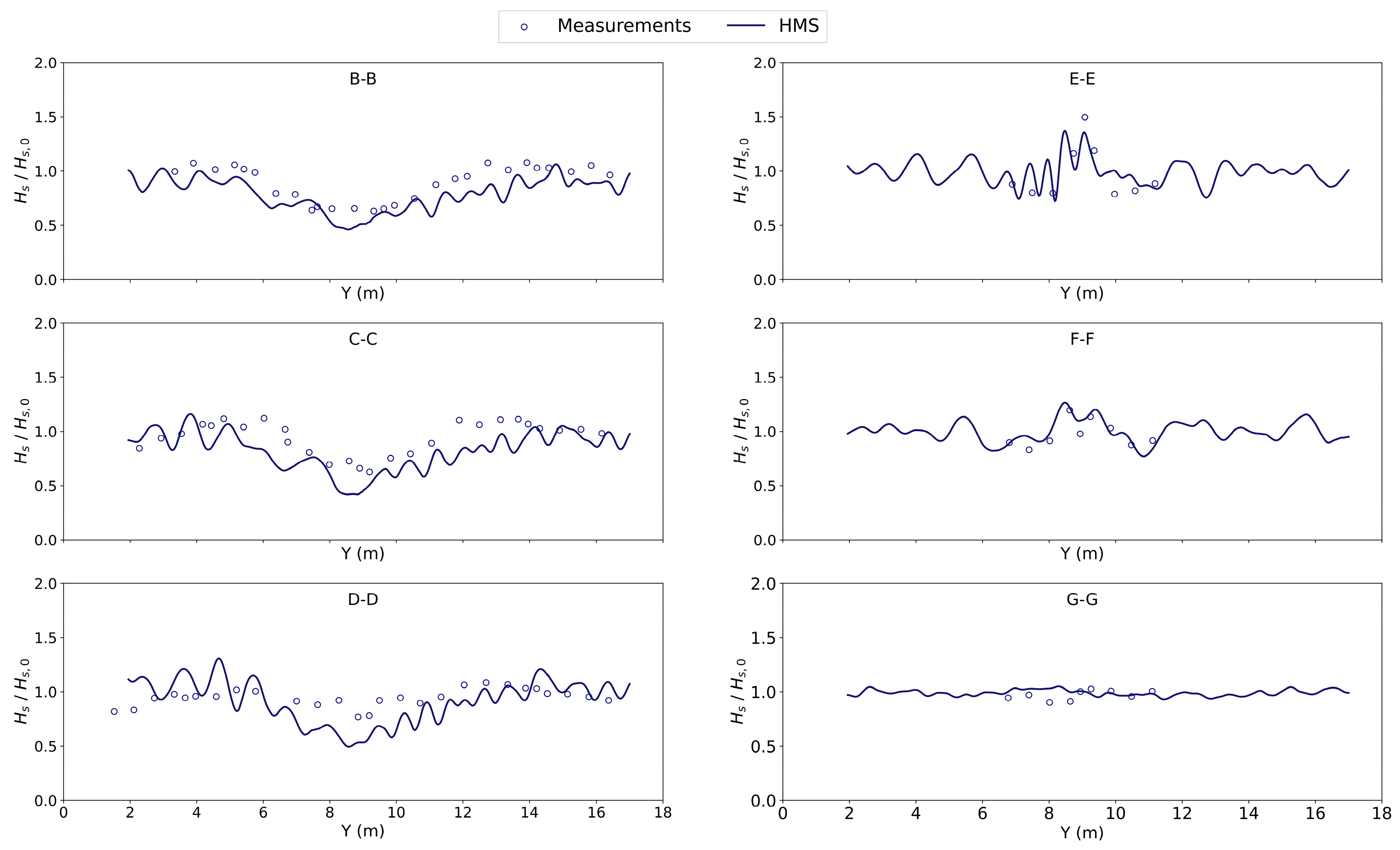
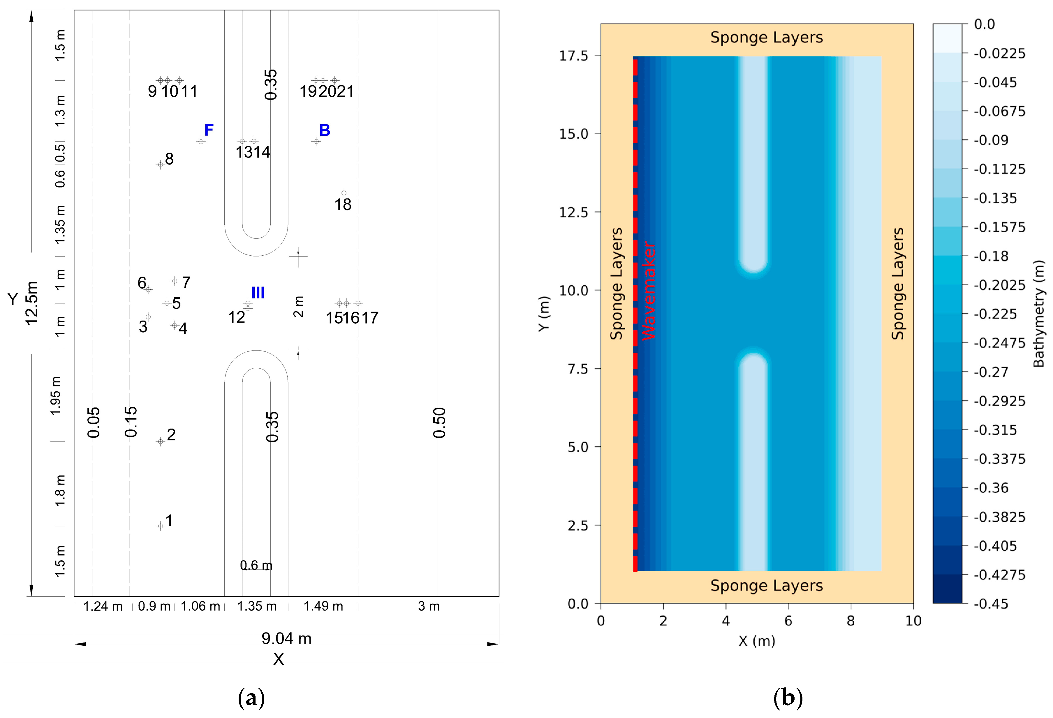
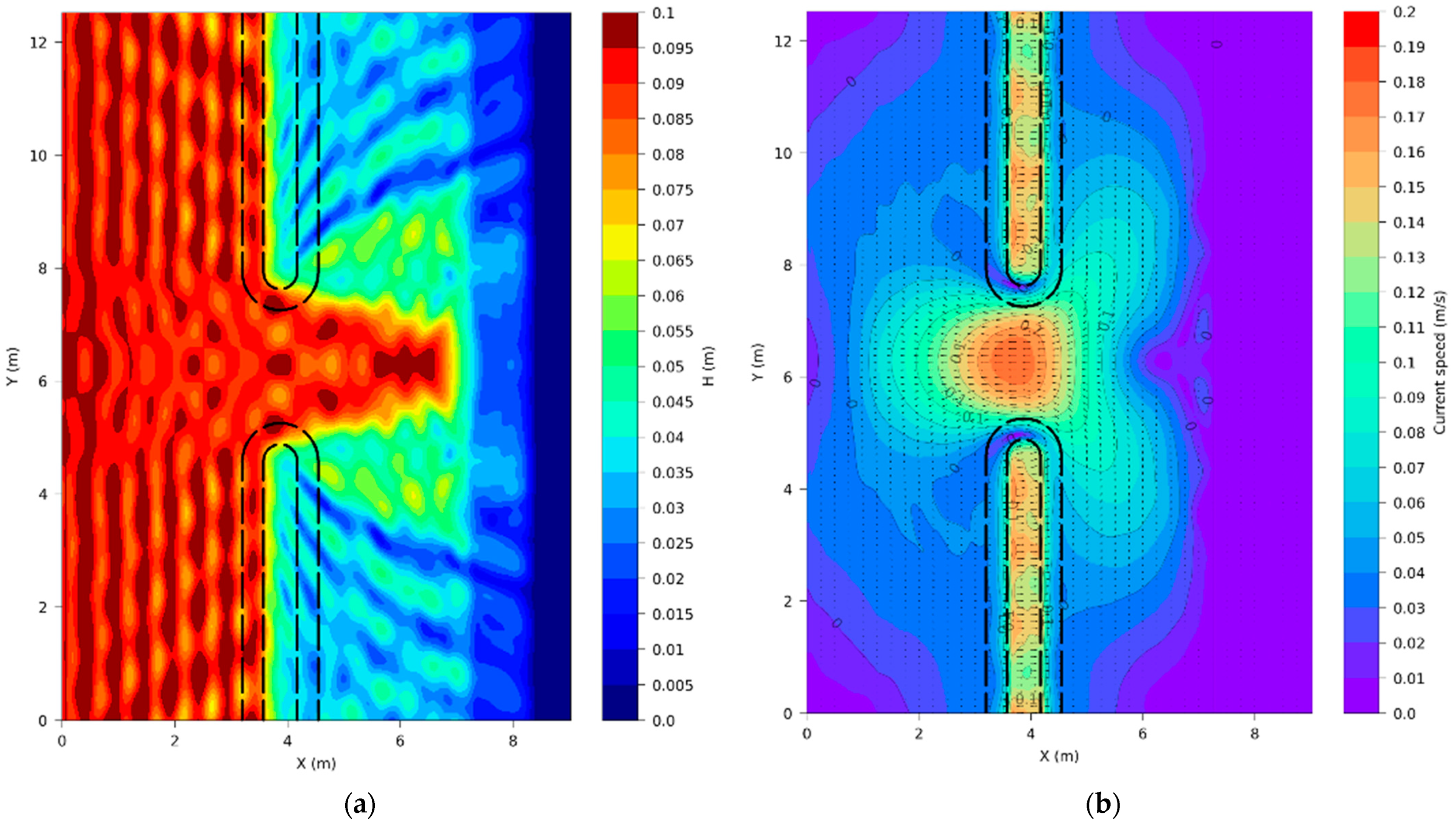
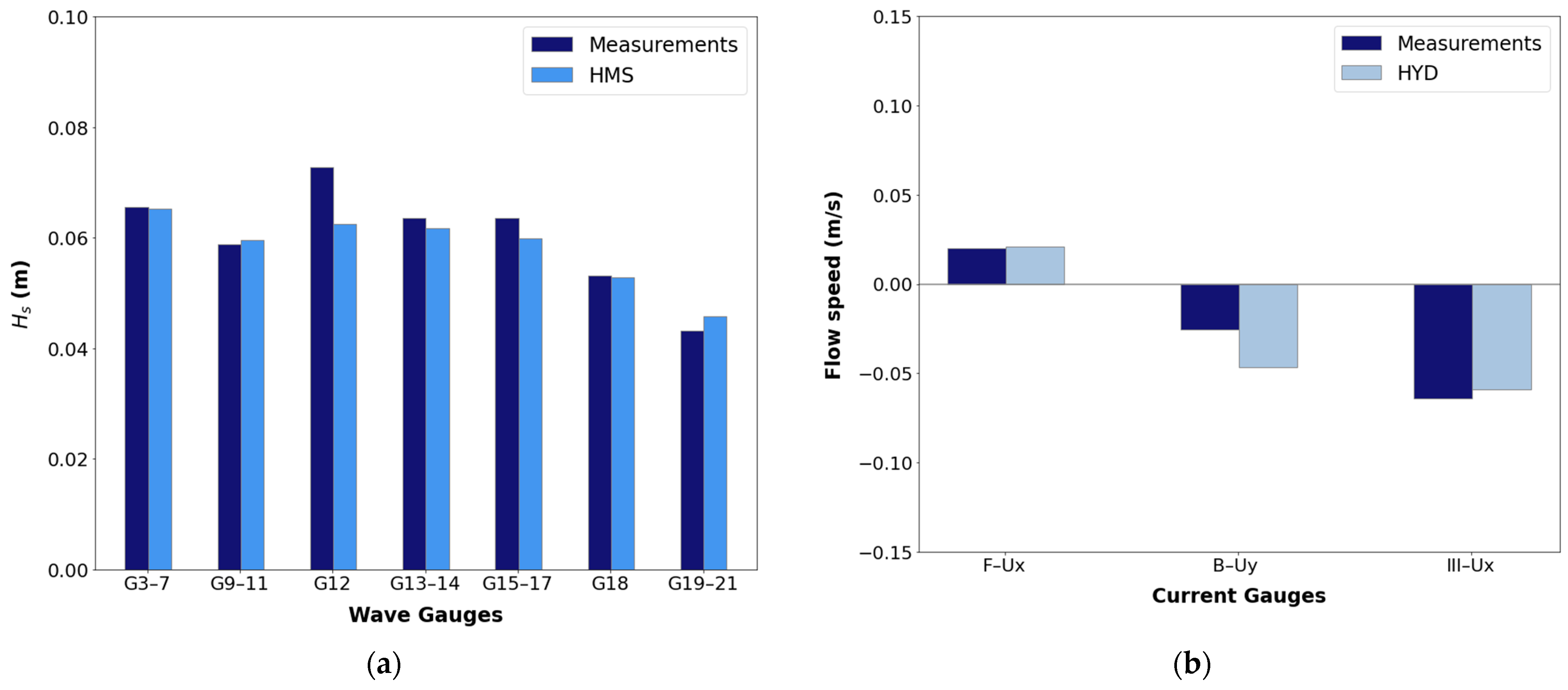
Hydrodynamic Conditions around Submerged Breakwaters [72]

A series of 3D experiments on low-crested structures were carried out in the 9.7 m long by 12.5 m wide wave basin at Aalborg University, Denmark [72], aiming to study the wave transformation and hydrodynamics around several configurations of low-crested structures. One of the layouts examined entails a symmetric arrangement of two detached breakwaters separated by a gap. For more details on the layout and incident wave characteristics, the reader is referred to [72,73]. Out of the several examined configurations, the layout of submerged breakwaters with a wide berm was selected to be simulated with the present numerical models. In the physical experiment, the breakwaters were constructed with a rock armor layer on a core with slopes designed in a 1:2 ratio. The structures were built over a horizontal bottom and were backed by an absorbing beach consisting of crushed stones placed on a 1:5 bed slope. The experimental layout of said case, superimposed with the positions of the wave gauges and the current speed measuring stations, is shown in Figure 8.
Test 37, concerning wave transformation and wave-generated currents in the vicinity of the wide-berm submerged breakwaters separated by a gap, is selected to be reproduced numerically with the combination of the HMS and HYD models. The incident wave characteristics are given in Table 3.
The numerical grid used in the wave propagation and hydrodynamic simulations consisted of 400 and 740 cells in the x- and y-directions, respectively, with a constant cell size of 0.025 m in both directions. It is noted that for the irregular multidirectional case, 26 wave components were used to discretize the wave spectrum, with 13 directional wave components. To better capture the quantity of the wave energy dissipation in the HMS model, due to the presence of the submerged breakwaters, the parameters of the Battjes and Jansen [60] breaking criterion are adjusted to the following values ( a = 0.81, γ 1 = 1.0, γ 2 = 0.8) for both cases. It is noted that the manning coefficient was set as a constant.
Figure 9 depicts maps of the computed wave field and the wave-generated currents at the vicinity of the submerged breakwaters for the regular sea state (Test 37). The wave diffraction, as well as the energy dissipation at the lee of the structure location, can be easily identified in Figure 9. The current speed pattern in general is onshore and directed over the submerged breakwater and offshore and directed (towards the wave generator) at the breakwater gap. The flow patterns are in good agreement qualitatively compared to the observations of the laboratory experiment as reported in [73].
The comparison between the computed wave heights and current speeds at selected measuring gauges with the experimental measurements is shown in Figure 10.
As far as the wave heights are concerned, a good comparison between experimental measurements and simulation results is observed in the selected wave gauges, with a Pearson correlation coefficient of R = 0.852. In particular, a slight overprediction is observed in the gauges offshore the submerged breakwater (G9–11), signifying that the model overcompensates the estimation of partial wave reflection. The computed wave heights at the lee of the breakwater (G18 and G19–21) remain lower than the measured values. Particularly, despite exploring several values for the breaking parameters the wave heights at the lee of the breakwater are still underpredicted by the model. This may be attributed to the model’s inability to simulate wave–wave and wave–current interactions.
As far as the current speeds are concerned, a satisfactory agreement is achieved between computed values and experimental measurements. The current speed values are slightly overpredicted by HYD at gauges F and III, while a near-perfect agreement is achieved in gauge B.
In a similar manner, Figure 11 presents a comparison between the computed wave heights and current speeds at selected measuring gauges and the experimental measurements for Test 35, which corresponds to an irregular multidirectional Jonswap spectrum source function.
A very good agreement is identified between the experimental measurements and the numerical results from HMS and HYD. For the wave height results, the largest discrepancy is observed in station 12, located in the middle of the breakwater gap. In contrast to the case of regular waves, the model captures the correct order of magnitude of the wave energy dissipation at wave gauges 19–21 located at the lee of the breakwater. As far as the flow speeds are concerned, a near-perfect agreement is observed for the U-velocity component in stations F and III, whereas the model slightly overpredicts. Overall, the performance of the HYD model forced with the radiation stresses calculated by HMS is deemed very satisfactory for a complex case where wave–structure interaction dominates the wave transformation processes and hydrodynamics for both regular and irregular sea states.

3.3. Validation of the Sediment Transport Model (SDT)

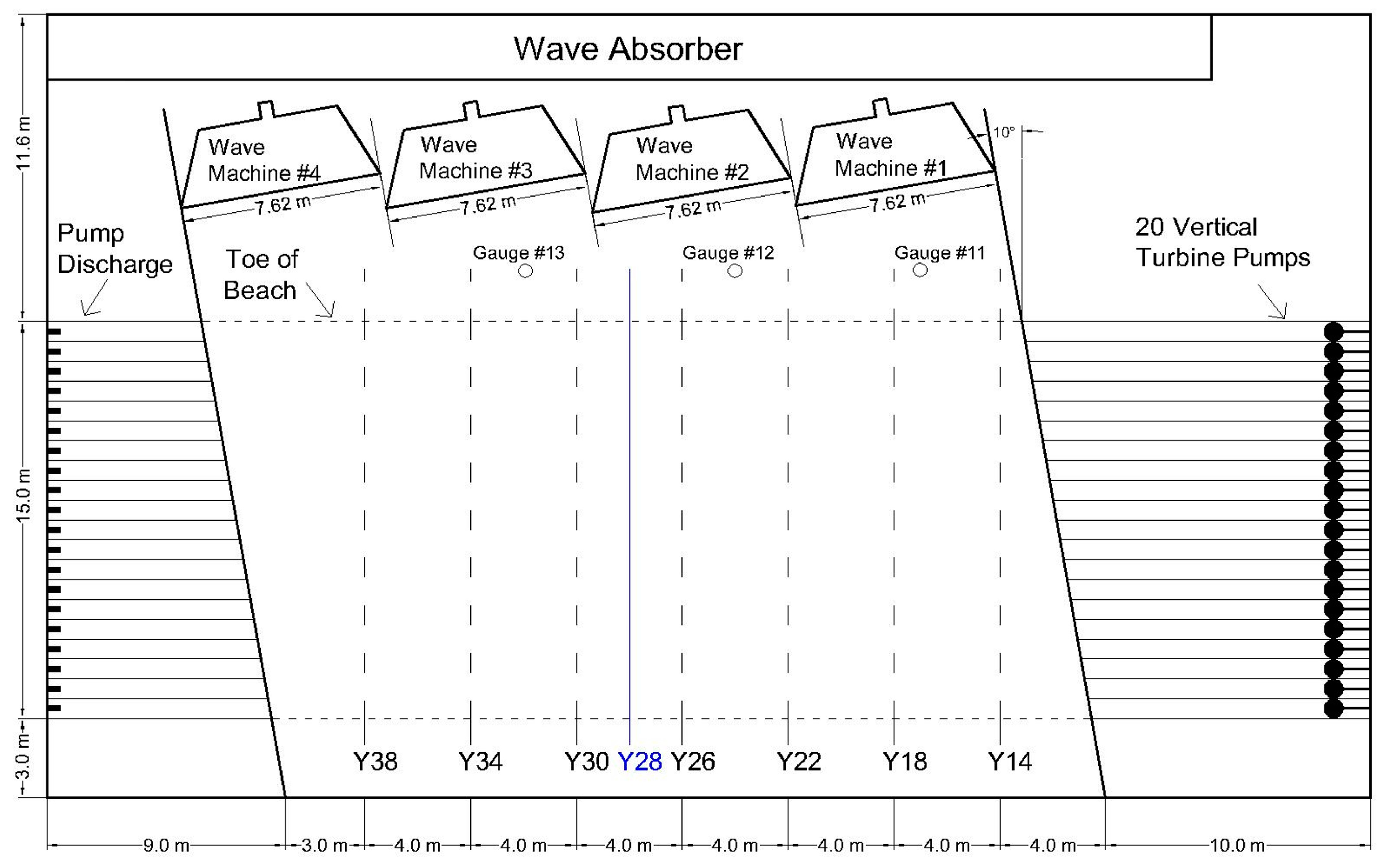
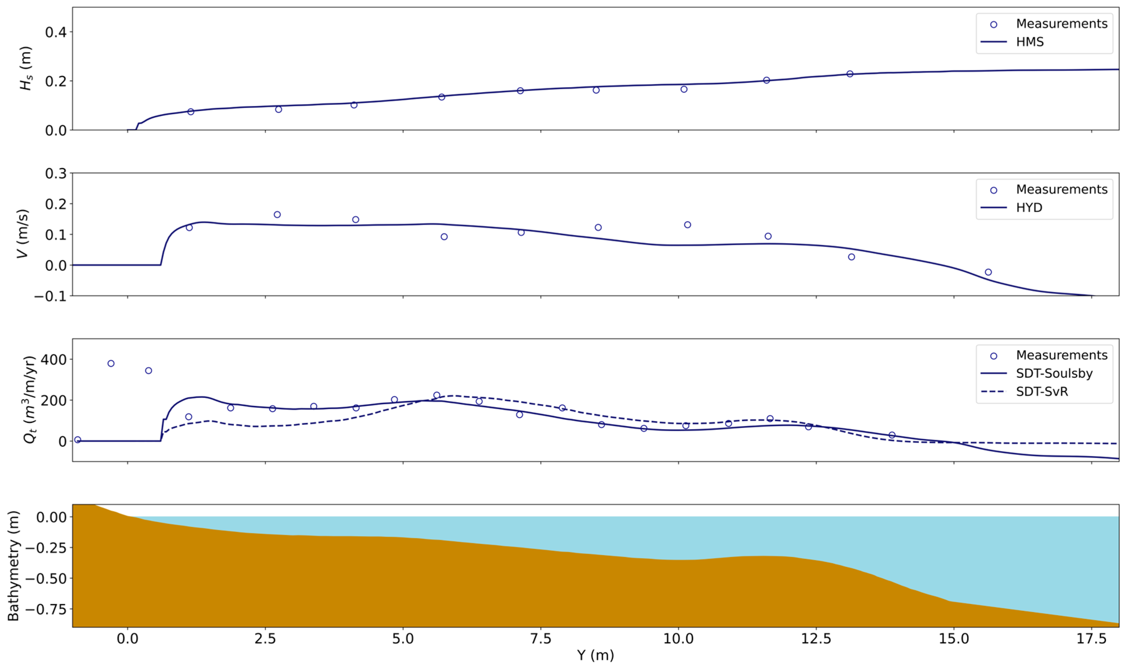
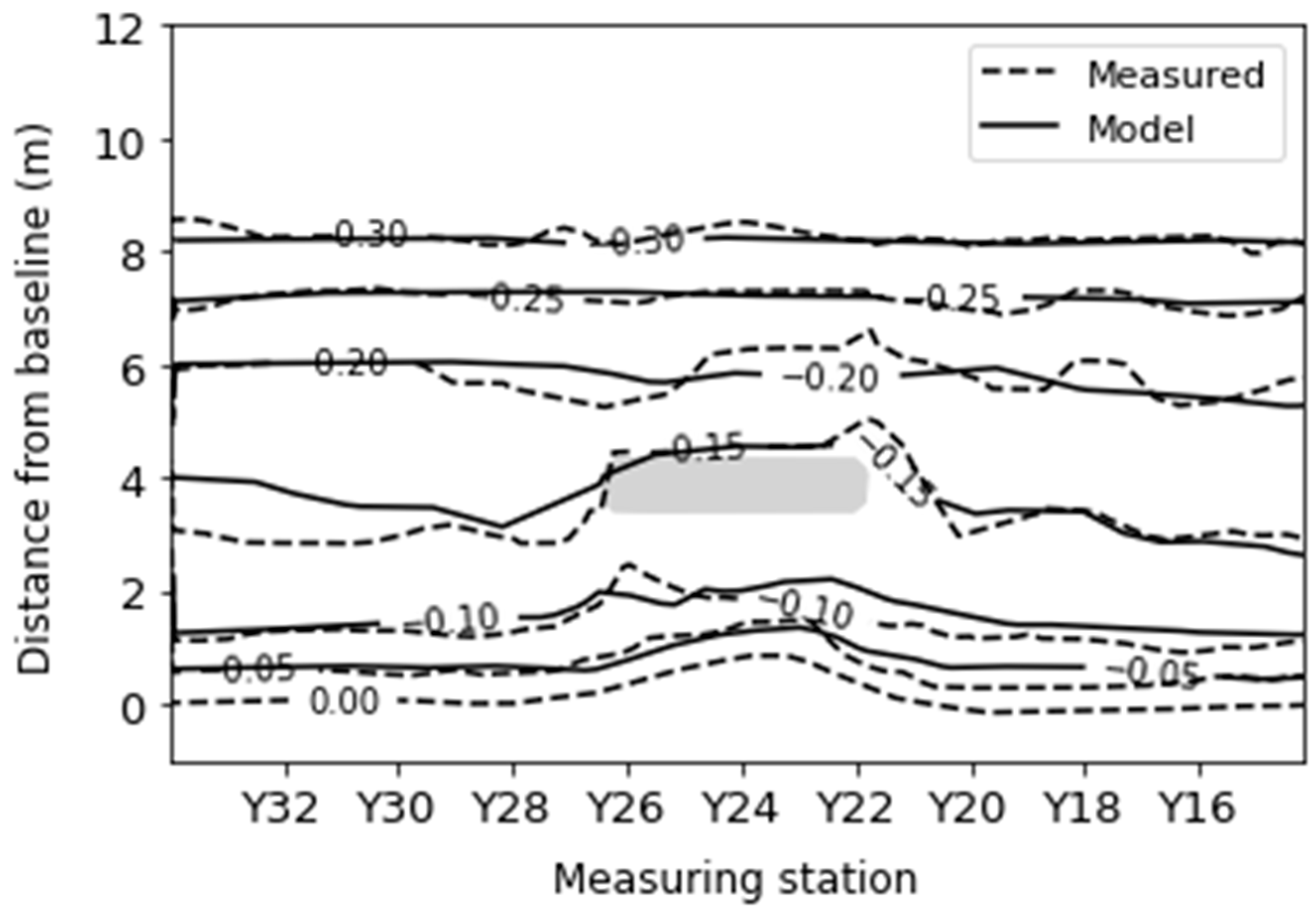
Longshore Currents and Sediment Transport in a Large-Scale Movable Bed Experiment [74]

In this subsection, we validate the SDT model using the experiment described in [74], concerning longshore currents and sediment transport in a two-dimensional movable bed large-scale experiment (LSTF). The experiments were conducted at the Coastal and Hydraulics Laboratory of the U.S. Army Engineer Research and Development Center in Vicksburg, with a wave basin 30 m long, 50 m wide, and 1.4 m deep. A movable bed beach made of quartz sand with a median sediment diameter of d50 = 0.15 mm, constructed atop a concrete fixed bed beach, was placed in the central region of the facility. The initial beach profile was constructed to form an “equilibrium state”. The test reproduced herein with the sequence of the HMS, HYD, and SDT models is BC1, concerning the oblique incidence of long-crested irregular waves with a TMA spectrum source function. The wave characteristics over the horizontal bottom of a 0.706 m depth were T p = 1.468 s and H s = 0.225 m, and the angle of wave incidence was 10°. The duration of the test was 165 min, and the still water depth at the wavemaker was 0.9 m. The wave characteristics, longshore current speeds, and sediment transport rates were measured along several transversal sections at 2 m intervals. The experimental layout of the LSTF experiment is shown in Figure 12. Due to the negligible alongshore variability of the beach, the physical quantities of waves, currents, and sediment transport are considered constant along the transversal sections; therefore, section Y28 was selected to export the wave, current, and sediment transport characteristics in the numerical model simulations.
The grid used in the numerical simulations is 1150 cells long and 508 cells wide, with a constant spatial step in both directions equal to 0.05 m. A manning coefficient of n = 0.012 s/m1/3 is set constant throughout the domain. In the wave, model sponge layers with a width of 5 m are placed at the lateral boundaries and directly behind the wavemaker to minimize unwanted reflections from the lateral boundaries of the domain. For the SDT simulations, two sediment transport formulas by Soulsby and Van Rijn (denoted SvR) and Soulsby’s bedload formula (denoted Soulsby) are utilized to intercompare the results. The simulated significant wave height, longshore current speed, and sediment transport rate are compiled in Figure 13, in comparison to the experimental data. It is noted that the point of Y = 0 m is the shoreline position.
For the simulated significant wave heights along profile Y28, a near-perfect agreement with the experimental measurements is observed. A small discrepancy can only be located after the first bar (at Y = 10.5 m) where the numerical model slightly underpredicts the energy dissipation and, consequently, overestimates the significant wave height. The corresponding longshore current speed (V) calculated by the HYD model also agrees fairly well with the experimental measurements. The largest discrepancy is, once again, identified directly after the abrupt change in the bathymetry after the first bar, coinciding with the wave model results in this particular area.
Finally, the sediment transport rates simulated with the SDT model agree fairly well with the experimental measurements. Comparing the two distinct sediment transport formulas, it can be deduced that the Soulsby bedload formula performs better than the SvR total load formula, especially at the breaker zone near the shoreline (from Y = 0 m up until Y = 5 m). The better performance of this formula may be attributed to the criterion of incipient threshold motion, which considers the bed shear stress due to the combined action of waves and currents for the Soulsby formula instead of the threshold current speed [63] criterion used in the SvR formula. Consequently, the latter formula more closely follows the longshore current speed distribution and, therefore, underpredicts the sediment transport rates around this area. It is noteworthy that the model is not capable of capturing the complex sediment dynamics in the swash zone and, as a future research initiative, the inclusion of sediment transport formulas (i.e., as the one presented by [76]) valid for the swash zone will be incorporated. In general, the performance of the sediment transport model is highly satisfactory in the nearshore and the beaker zone but has less accuracy in the swash zone.
Having validated the integrated model for the baseline test BC1, herein, the test T1C1 by [74] is reproduced, referring to a detached breakwater 4 m long placed at a distance of 4 m from the initial shoreline coinciding with the baseline. The tips of the breakwater were located between stations Y26 and Y22, the positions of which are shown in Figure 12. This test will serve to validate the capability of the integrated model in simulating the coastal processes and the bed evolution in the vicinity of a breakwater. The following wave characteristics were generated at the wavemaker: H s = 0.219 m, T p = 1.442 s, and θ 0 = 6.5° with respect to the normal shore. The extent and configuration of the numerical grid were identical to the baseline test BC1, and the placement of the breakwater is illustrated in Figure 14. It is noted that the area enclosed within the orange polygon depicts where the morphological bed evolution results will be evaluated.
The total duration of the simulation was 185 min, as was the case in the physical experiment. Since the simulation duration was not overly excessive, no morphological acceleration factor was employed in the SDT model. Figure 15 depicts the bed evolution at the evaluation area in the vicinity of the breakwater. Comparing the predicted bed elevations, it can be deduced that the model results agree fairly well with the experimental measurements. In particular, the salient formed at the lee of the breakwater is reproduced well by the numerical model. The largest discrepancies between model results and measurements are identified at the inner surf zone (i.e., at a bed elevation of about −0.15 m), where the model slightly underpredicts the observed erosion. A slighter underprediction of the extent of the erosion is also identified at the right opening of the breakwater. Overall, the performance of the model in predicting the coastal bed evolution in the vicinity of a coastal protection structure is deemed quite satisfactory.

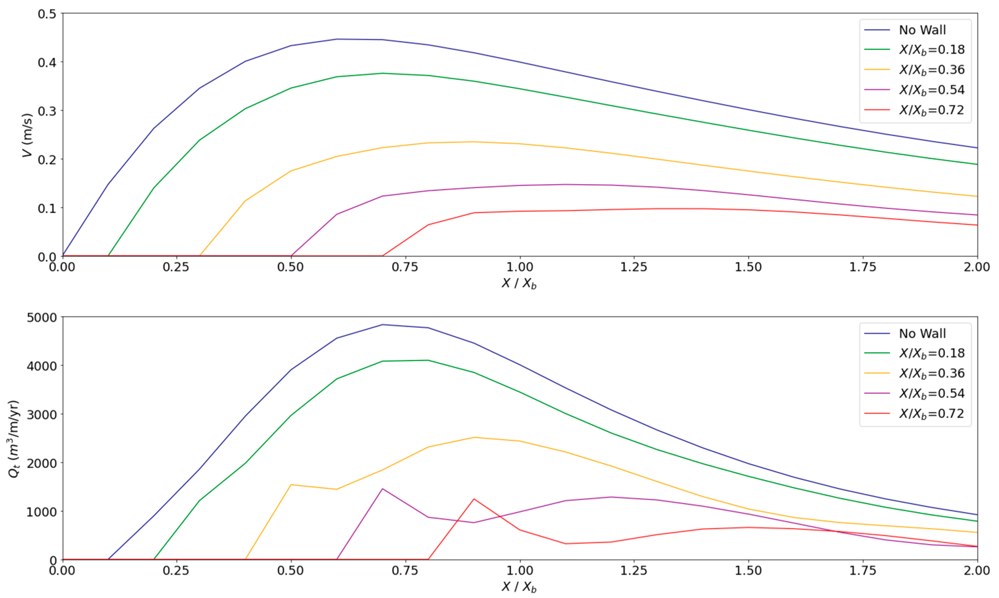
4. Numerical Evaluation of the Effect of Wave Reflection on Longshore Coastal Processes

In this section, a numerical evaluation is carried out to assess how wave reflection caused by the presence of a seawall affects the longshore current and corresponding sediment transport rates. The main inspiration of this numerical study is the work by [40], who derived an analytical solution to predict the time and depth-averaged longshore and cross-shore hydrodynamics for a plane-sloping beach backed by a seawall for regular waves. The authors rigorously studied the effect of a seawall placed at varying positions within the surf zone for several wave conditions and beach slopes for the case of spilling breakers and concluded that the position of the seawall was critical in either increasing or decreasing the magnitude of the longshore flow rate and sediment transport.
The integrated model is hereafter applied for two incident sea states as presented in Table 4 with an angle of wave incidence compared to the normal shore of a 0 = 20° for two distinct cases of sloping beds with a steep slope of 1:10 and 1:50 covering the cases of both spilling and plunging breakers. Irregular unidirectional waves with a JONSWAP spectrum were generated in the wave model in an attempt to expand on the work by [40] and provide some initial insights on the effect of wave reflection on coastal processes under irregular sea states. Consequently, the notable differences between this numerical investigation and the work by [40] are the consideration of irregular unidirectional sea states instead of regular waves and combinations of bed slope and sea state wave characteristics referring to spilling and plunging breakers.
In the numerical implementation, the maximum water depth at the wavemaker in both bed slope tests is 60 m, and a numerical grid of 1230 cells in the cross-shore and 1900 cells in the alongshore direction was constructed with a 2.5 m discretization step in both directions. In the wave model, sponge layers with a width of 125 m are placed perimetrically to absorb the reflected wave energy in all four boundaries of the domain for all cases. A bottom friction coefficient with a manning coefficient of 0.02 s/m1/3 and a horizontal eddy viscosity coefficient of v h = 2 m2/s are set constant in the hydrodynamic model. For the sediment transport model, the sediment transport formula by Soulsby and Van Rijn (SvR) is employed. Simulations are conducted at five different positions along the seawall for each bed slope, one case considering the plane-sloping beach without the vertical seawall and four cases considering the varying placement of the seawall within the surf zone. The placement of the seawall is given as a non-dimensional quantity of X / X b , with X b being the distance of the breaker line from the coastline. It is noted that since the examined cases refer to irregular waves, distinguishing the breaker point becomes more intricate due to the more saturated surf zone in contrast to the case for regular waves. Therefore, the position of X b is considered to be the one with the highest value of the fraction of breaking waves Q b for the case of the beach without the presence of the seawall. Figure 16 presents the longshore current speed and longshore sediment transport rate at a cross-shore section for the case without the seawall and for four positions of the seawall within the surf zone for the bed with a slope of 1:10 for Case 1a, whereas Figure 17 refers to Case 1b, respectively.
In both Figures, it can be deduced that the magnitude of the longshore current speeds decreases as the seawall is placed further seaward. In general, the same behavior is observed for the sediment transport rates, with a more acute peak appearing close to the face of the seawall for the cases of X / X b ≥ 0.36, especially for Case 1b, which is associated with more energetic sea states.
Figure 18 and Figure 19, in turn, showcase the computed longshore currents and sediment transport rates for the bed with a slope of 1:50 (Case 2a and 2b, respectively). In general, the longshore current seems to gradually decrease for all cases with a seawall placed within the surf zone for both cases of incident sea states. In the case of X / X b = 0.18, where the seawall is placed closer to the shoreline, the longshore current speed is almost unaffected by the seawall since by that point, the incident waves have dissipated the largest proportion of their energy due to breaking. Additionally, the peaks of the longshore current move offshore due to the placement of the seawall. It is noted that similar to the steeper bed slope, the longshore current speeds demonstrate a “smooth” behavior without fluctuations. The sediment transport rates paint a different picture with noticeable fluctuations and a significant sensitivity to the relative position of the seawall. Particularly, for Case 2a and the relative position X / X b = 0.72, two peaks can be clearly identified with the highest magnitude of the sediment transport rate compared to the case without the seawall. For Case 2b, the fluctuations exhibit peaks that are larger than the case without a seawall starting from X / X b = 0.54. This behavior is attributed to the contribution of the near-bed wave orbital velocity, which varies due to the formation of the standing waves and, consequently, affects the sediment transport potential. It also indicates that the contribution of the reflected waves in milder bed slopes plays a pivotal role in coastal morphodynamics, showcasing the importance of employing a phase-resolving wave model as the main driver of the integrated models.
Overall, the conclusions obtained from this parametric numerical study are in agreement with the ones drawn by [40], who also identified that for the steeper slopes, the longshore current and sediment transport rates clearly decreased due to the placement of the seawall, while for milder bed slopes, the flow rates showcased fluctuations with local maxima and minima, depending on the position of the nodes and antinodes of the standing wave patterns. For the two incident sea states examined, the same patterns can be observed, indicating that the observed fluctuations of the sediment transport rates are predominately dependent on the bed slope. Summarily, this numerical study further indicates a clear influence and contribution of the seawall in longshore sediment transport processes but does not clearly indicate whether wave reflection contributes to a significant increase or decrease in long-term erosion. This is attributed to the sensitivity of the problem on the incident wave conditions, beach geometry, and placement of the seawall, as has been noted by [40]. Field measurements in real-field applications (e.g., such as the ones shown in [39]) can contribute to providing more insights into the effect of seawalls in longshore hydrodynamics and morphodynamics, especially in more complex beach configurations, to study the patterns of the wave-generated currents and how other parameters (e.g., angle of wave attack) can potentially affect the long-term morphological bed evolution.

5. Conclusions

This study presents an integrated approach using three numerical models: HMS for wave transformation, HYD for hydrodynamics, and SDT for sediment transport to simulate and investigate coastal processes. All the individual models have been validated in several experimental cases, covering application ranging from wave energy dissipation due to bathymetric breaking and bottom friction, hydrodynamics at the vicinity of coastal protection works, and sediment dynamics in equilibrium beach profiles. The models operate in a “one-way” coupling manner and are sequentially applied. Specifically, HMS simulates the nearshore wave field, providing radiation stresses as input to HYD, which calculates the nearshore hydrodynamic field. The resultant wave and current data are then utilized by SDT to compute sediment transport and bed evolution rates. The latter can be used to generate a new bathymetry, and further cycles of simulations can be carried out for a set duration. This approach can be applied to any coastal area with or without the presence of coastal and harbor works, bearing in mind the following capabilities and limitations of each model.
The proposed HMS model can simulate the propagation of regular and irregular waves and describe all the dominant transformation phenomena that take place in coastal areas, such as shoaling, refraction, diffraction, reflection, and energy loss due to depth-induced breaking and bottom friction. Through comprehensive validation against three benchmark experiments, including wave decay due to bottom friction and irregular wave breaking on sloping beaches, the wave model demonstrated commendable efficacy in replicating critical wave transformation processes. Nevertheless, some discrepancies were observed that can be attributed to its inability to simulate wave–wave and wave–current interactions. Having validated the wave model, the validation of the HYD model was then carried out for a case of wave-generated currents of wide-berm submerged breakwaters separated by a gap. The HYD model exhibited a robust performance in a challenging problem involving wave–structure interaction. The comparison with the experimental data showcased good agreement in current speeds, emphasizing the model’s ability to simulate complex hydrodynamic phenomena. However, it should be noted that HYD solves the Reynolds-averaged Navier–Stokes equations, thus only providing the depth-averaged current velocities in the two horizontal directions and thus not capturing 3D hydrodynamic effects.
The proposed SDT model demonstrated satisfactory performance in nearshore and breaker zone conditions. Validation against experimental measurements revealed very good agreement and fairly accurate predictions of longshore sediment transport. The two sediment transport formulas that were evaluated in the framework of this research exemplified a good performance in the surf zone but underestimated the sediment transport rates in the swash zone, highlighting the need for incorporating sediment transport formulas specifically tailored for such dynamic environments.
The integration of the HMS, HYD, and SDT models proved effective overall in simulating the considered coastal processes. Validation against experimental data, including a demanding test case involving a detached breakwater, demonstrated the integrated model’s ability to predict the coastal bed evolution satisfactorily. This underscores its potential as a valuable tool for optimizing coastal protection schemes and mitigating erosion risks.
Moreover, a numerical investigation was carried out to assess if the wave reflection of irregular unidirectional waves potentially affects longshore hydrodynamics and sediment transport rates. Two plane-sloping beach configurations with a steeper slope of 1:10 and a milder one of 1:50 were examined for a case of spilling and plunging breakers, respectively. The conclusions drawn from this numerical investigation are that for the case of the steeper bed slope, the longshore current speed and sediment transport rates decrease in the presence of the seawall, while for the milder bed slope, the width of the breaker zone increases, leading to increased magnitude of the peak sediment transport rate when the seawall is placed at about 0.7 times the distance of the breaker point to the shoreline position. It is noted that these findings are in agreement with the ones obtained by [40], who developed an analytical solution to study the hydrodynamics and sediment transport for regular waves in a beach backed by a seawall. Additionally, our numerical investigation highlighted that the presence of reflected waves, especially in milder bed slopes, plays a pivotal role in coastal morphodynamics, underscoring the importance of employing a phase-resolving wave model that takes into account the reflection, as the main driver of the integrated modeling of coastal processes.
Future research efforts will focus on incorporating wave–current interactions and sediment transport formulas tailored for swash zone dynamics to enhance the accuracy of the integrated model. Furthermore, field measurements in real-world applications are of utmost importance to provide valuable data for further model validation, as well as to deepen our understanding of the reflection effects on coastal morphodynamics, aiding significantly in informed decision making for coastal protection.

Author Contributions

Conceptualization, M.K.C., A.G.P. and A.S.M.; methodology, M.K.C., A.G.P. and A.S.M.; software, M.K.C., A.G.P. and A.S.M.; validation, M.K.C., A.G.P. and A.S.M.; formal analysis, M.K.C., A.G.P. and A.S.M.; investigation, M.K.C., A.G.P. and A.S.M.; resources, M.K.C., A.G.P. and A.S.M.; data curation, M.K.C., A.G.P. and A.S.M.; writing—original draft preparation, M.K.C., A.G.P. and A.S.M.; writing—review and editing, M.K.C., A.G.P. and A.S.M.; visualization, M.K.C., A.G.P. and A.S.M.; supervision, M.K.C., A.G.P. and A.S.M.; project administration, M.K.C., A.G.P. and A.S.M.; funding acquisition, M.K.C., A.G.P. and A.S.M. All authors have read and agreed to the published version of the manuscript.

Funding

This research received no external funding.

Informed Consent Statement

Not applicable.

Data Availability Statement

The data presented in this study are available on request from the corresponding author.

Conflicts of Interest

The authors declare no conflicts of interest.

References

  1. Roelvink, D.; Reniers, A. A Guide to Modeling Coastal Morphology, 1st ed.; Word Scientific: Singapore, 2012; p. 292. [Google Scholar]
  2. Brown, J.M.; Davies, A.G. Methods for medium-term prediction of the net sediment transport by waves and currents in complex coastal regions. Cont. Shelf Res. 2009, 29, 1502–1514. [Google Scholar] [CrossRef]
  3. Gad, F.-K.; Hatiris, G.-A.; Loukaidi, V.; Dimitriadou, S.; Drakopoulou, P.; Sioulas, A.; Kapsimalis, V. Long-Term Shoreline Displacements and Coastal Morphodynamic Pattern of North Rhodes Island, Greece. Water 2018, 10, 849. [Google Scholar] [CrossRef]
  4. Papadimitriou, A.; Panagopoulos, L.; Chondros, M.; Tsoukala, V. A wave input-reduction method incorporating initiation of sediment motion. J. Mar. Sci. Eng. 2020, 8, 597. [Google Scholar] [CrossRef]
  5. Papadimitriou, A.; Chondros, M.; Metallinos, A.; Tsoukala, V. Accelerating Predictions of Morphological Bed Evolution by Combining Numerical Modelling and Artificial Neural Networks. J. Mar. Sci. Eng. 2022, 10, 1621. [Google Scholar] [CrossRef]
  6. Malliouri, D.I.; Petrakis, S.; Vandarakis, D.; Moraitis, V.; Goulas, T.; Hatiris, G.A.; Drakopoulou, P.; Kapsimalis, V. A Chronology-Based Wave Input Reduction Technique for Simulations of Long-Term Coastal Morphological Changes: An Application to the Beach of Mastichari, Kos Island, Greece. Water 2023, 15, 389. [Google Scholar] [CrossRef]
  7. Latteux, B. Harbour design including sedimentological problems using mainly numerical techniques. In Proceedings of the 17th International Conference on Coastal Engineering, Sydney, Australia, 23–28 March 1980. [Google Scholar] [CrossRef]
  8. Liu, P.L.F.; Losada, I.J. Wave propagation modeling in coastal engineering. J. Hydraul. Res. 2002, 40, 229–240. [Google Scholar] [CrossRef]
  9. Ilic, S.; van der Westhuysen, A.J.; Roelvink, J.A.; Chadwick, A.J. Multidirectional wave transformation around detached breakwaters. Coast. Eng. 2007, 54, 775–789. [Google Scholar] [CrossRef]
  10. Du, Y.; Pan, S.; Chen, Y. Modelling the effect of wave overtopping on nearshore hydrodynamics and morphodynamics around shore-parallel breakwaters. Coast. Eng. 2010, 57, 812–826. [Google Scholar] [CrossRef]
  11. Nam, P.T.; Larson, M.; Hanson, H.; Hoan, L.X. A numerical model of beach morphological evolution due to waves and currents in the vicinity of coastal structures. Coast. Eng. 2011, 58, 863–876. [Google Scholar] [CrossRef]
  12. Postacchini, M.; Russo, A.; Carniel, S.; Brocchini, M. Assessing the Hydro-Morphodynamic Response of a Beach Protected by Detached, Impermeable, Submerged Breakwaters: A Numerical Approach. J. Coast. Res. 2016, 32, 590–602. [Google Scholar] [CrossRef]
  13. Karambas, T.V.; Samaras, A.G. An integrated numerical model for the design of coastal protection structures. J. Mar. Sci. Eng. 2017, 5, 50. [Google Scholar] [CrossRef]
  14. Ranasinghe, R.S. Modelling of waves and wave-induced currents in the vicinity of submerged structures under regular waves using nonlinear wave-current models. Ocean Eng. 2022, 247, 110707. [Google Scholar] [CrossRef]
  15. Afentoulis, V.; Papadimitriou, A.; Belibassakis, K.; Tsoukala, V. A coupled model for sediment transport dynamics and prediction of seabed morphology with application to 1DH/2DH coastal engineering problems. Oceanologia 2022, 64, 514–534. [Google Scholar] [CrossRef]
  16. Badiei, P.; Kamphuis, J.W.; Hamilton, D.G. Physical experiments on the effects of groins on shore morphology. In Proceedings of the 24th International Conference on Coastal Engineering, Kobe, Japan, 23–28 October 1994. [Google Scholar] [CrossRef]
  17. Ming, D.; Chiew, Y.-M. Shoreline Changes behind Detached Breakwater. J. Waterw. Port Coast. Ocean Eng. 2000, 126, 63–70. [Google Scholar] [CrossRef]
  18. Mory, M.; Hamm, L. Wave height, setup and currents around a detached breakwater submitted to regular or random wave forcing. Coast. Eng. 1997, 31, 77–96. [Google Scholar] [CrossRef]
  19. Lorenzoni, C.; Postacchini, M.; Brocchini, M.; Mancinelli, A. Experimental study of the short-term efficiency of different breakwater configurations on beach protection. J. Ocean Eng. Mar. Energy 2016, 2, 195–210. [Google Scholar] [CrossRef]
  20. Metallinos, A.S.; Klonaris, G.T.; Memos, C.D.; Dimas, A.A. Hydrodynamic conditions in a submerged porous breakwater. Ocean Eng. 2019, 172, 712–725. [Google Scholar] [CrossRef]
  21. Klonaris, G.T.; Metallinos, A.S.; Memos, C.D.; Galani, K.A. Experimental and numerical investigation of bed morphology in the lee of porous submerged breakwaters. Coast. Eng. 2020, 155, 103591. [Google Scholar] [CrossRef]
  22. Yu, Y.X.; Liu, S.X.; Li, Y.S.; Wai, O.W.H. Refraction and diffraction of random waves through breakwater. Ocean Eng. 2000, 27, 489–509. [Google Scholar] [CrossRef]
  23. Bos, K.J.; Roelvink, J.A.; Dingemans, M.W. Modelling the impact of detached breakwaters on the coast. In Proceedings of the 25th International Conference on Coastal Engineering, Orlando, FL, USA, 2–6 September 1996. [Google Scholar] [CrossRef]
  24. Cáceres, I.; Sánchez-Arcilla, A.; Zanuttigh, B.; Lamberti, A.; Franco, L. Wave overtopping and induced currents at emergent low crested structures. Coast. Eng. 2005, 52, 931–947. [Google Scholar] [CrossRef]
  25. Klonaris, G.T.; Memos, C.D.; Drønen, N.K. High-Order Boussinesq-Type Model for Integrated Nearshore Dynamics. J. Waterw. Port Coast. Ocean. Eng. 2016, 142, 04016010. [Google Scholar] [CrossRef]
  26. Gallerano, F.; Cannata, G.; Palleschi, F. Hydrodynamic Effects Produced by Submerged Breakwaters in a Coastal Area with a Curvilinear Shoreline. J. Mar. Sci. Eng. 2019, 7, 337. [Google Scholar] [CrossRef]
  27. Do, J.D.; Jin, J.Y.; Hyun, S.K.; Jeong, W.M.; Chang, Y.S. Numerical investigation of the effect of wave diffraction on beach erosion/accretion at the Gangneung Harbor, Korea. J. Hydro-Environ. Res. 2020, 29, 31–44. [Google Scholar] [CrossRef]
  28. Metallinos, A.; Chondros, M.; Papadimitriou, A. Simulating Nearshore Wave Processes Utilizing an Enhanced Boussinesq-Type Model. Modelling 2021, 2, 686–705. [Google Scholar] [CrossRef]
  29. Johnson, H.K.; Karambas, T.V.; Avgeris, I.; Zanuttigh, B.; Gonzalez-Marco, D.; Caceres, I. Modelling of waves and currents around submerged breakwaters. Coast. Eng. 2005, 52, 949–969. [Google Scholar] [CrossRef]
  30. Ruggiero, P. Impacts of shoreline armoring on sediment dynamics. In Puget Sound Shorelines and the Impacts of Armoring—Proceedings of a State of the Science Workshop, May 2009: U.S. Geological Survey Scientific Investigations Report 2010-5254; U.S. Geological Survey: Reston, VA, USA, 2009. [Google Scholar]
  31. Kraus, N.C.; McDougal, W.G. The effects of seawalls on the beach: Part I, an updated literature review. J. Coast. Res. 1996, 12, 691–701. [Google Scholar]
  32. Birkemeier, W.A. The Effect of Structures and Lake Level on Bluff and Shore Erosion in Berrien County, Michigan; US Army Corps Engineer, Coastal Engineering Research Center: Fort Belvoir, VA, USA, 1980. [Google Scholar]
  33. Macdonald, H.V.; Patterson, D.C. Beach response to coastal works Gold Coast, Australia. In Proceedings of the 19th International Conference on Coastal Engineering, Houston, TX, USA, 3–7 September 1984. [Google Scholar]
  34. Morton, R.A. Interactions of Storms, Seawalls, and Beaches of the Texas Coast. J. Coast. Res. 1988, 113–134. [Google Scholar]
  35. Dean, R.G. Coastal Armoring: Effects, Principles and Mitigation. In Proceedings of the 20th International Conference on Coastal Engineering, Taipei, Taiwan, 9–14 November 1986. [Google Scholar]
  36. Kamphuis, J.W.; Rakha, K.A.; Jui, J. Hydraulic model experiments on seawalls. In Proceedings of the 23th International Conference on Coastal Engineering, Venice, Italy, 4–9 October 1992. [Google Scholar]
  37. Rakha, K.A.; Kamphuis, J.W. Wave-induced currents in the vicinity of a seawall. Coast. Eng. 1997, 30, 23–52. [Google Scholar] [CrossRef]
  38. Rakha, K.A.; Kamphuis, J.W. A morphology model for an eroding beach backed by a seawall. Coast. Eng. 1997, 30, 53–75. [Google Scholar] [CrossRef]
  39. Miles, J.R.; Russell, P.E.; Huntley, D.A. Field measurements of sediment dynamics in front of a seawall. J. Coast. Res. 2001, 17, 195–206. [Google Scholar]
  40. Ruggiero, P.; McDougal, W.G. An analytic model for the prediction on wave setup, longshore currents and sediment transport on beaches with seawalls. Coast. Eng. 2001, 43, 161–182. [Google Scholar] [CrossRef]
  41. Holthuijsen, L.H. Waves in Oceanic and Coastal Waters; Cambridge University Press: Cambridge, UK, 2007; ISBN 9780511618536. [Google Scholar]
  42. Wei, G.; Kirby, J.T. Time-Dependent Numerical Code for Extended Boussinesq Equations. J. Waterw. Port Coast. Ocean. Eng. 1995, 121, 251–261. [Google Scholar] [CrossRef]
  43. Chondros, M.K.; Memos, C.D. A 2DH nonlinear Boussinesq-type wave model of improved dispersion, shoaling, and wave generation characteristics. Coast. Eng. 2014, 91, 99–122. [Google Scholar] [CrossRef]
  44. Karambas, T.V.; Memos, C.D. A 2DH post-Boussinesq model for weakly nonlinear fully dispersive water waves. In Proceedings of the 31st International Conference on Coastal Engineering, Hamburg, Germany, 31 August–5 September 2008. [Google Scholar]
  45. Nwogu, O. Alternative Form of Boussinesq Equations for Nearshore Wave Propagation. J. Waterw. Port Coast. Ocean Eng. 1993, 119, 618–638. [Google Scholar] [CrossRef]
  46. Kirby, J.T.; Dalrymple, R.A. A parabolic equation for the combined refraction diffraction of Stokes waves by mildly varying topography. J. Fluid Mech. 1983, 136, 453–466. [Google Scholar] [CrossRef]
  47. Li, B. An evolution equation for water waves. Coast. Eng. 1994, 23, 227–242. [Google Scholar] [CrossRef]
  48. Copeland, G.J.M. A practical alternative to the “mild-slope” wave equation. Coast. Eng. 1985, 9, 125–149. [Google Scholar] [CrossRef]
  49. Chondros, M.K.; Metallinos, A.S.; Memos, C.D.; Karambas, T.V.; Papadimitriou, A.G. Concerted nonlinear mild-slope wave models for enhanced simulation of coastal processes. Appl. Math. Model. 2021, 91, 508–529. [Google Scholar] [CrossRef]
  50. Gallerano, F.; Cannata, G.; De Gaudenzi, O.; Scarpone, S. Modeling Bed Evolution Using Weakly Coupled Phase-Resolving Wave Model and Wave-Averaged Sediment Transport Model. Coast. Eng. J. 2016, 58, 1650011. [Google Scholar] [CrossRef]
  51. Klonaris, G.T.; Memos, C.D.; Drønen, N.K.; Deigaard, R. Boussinesq-type modeling of sediment transport and coastal morphology. Coast. Eng. J. 2017, 59, 1750007-1–1750007-2. [Google Scholar] [CrossRef]
  52. Afentoulis, V.; Papadimitriou, A.; Benoit, M.; Tsoukala, V. Numerical Approaches for the Evaluation of Sediment Transport Mechanisms on a Shallow Sloping Sea Bottom. In Proceedings of the Design and Management of Port, Coastal and Offshore Works Conference, Athens, Greece, 8–11 May 2019. [Google Scholar]
  53. Tehranirad, B.; Kirby, J.T.; Shi, F. A Numerical Model for Tsunami-Induced Morphology Change. Pure Appl. Geophys. 2021, 178, 5031–5059. [Google Scholar] [CrossRef]
  54. Tsiaras, A.-C.; Karambas, T.; Koutsouvela, D. Design of Detached Emerged and Submerged Breakwaters for Coastal Protection: Development and Application of an Advanced Numerical Model. J. Waterw. Port Coast. Ocean. Eng. 2020, 146, 04020012. [Google Scholar] [CrossRef]
  55. Demirbilek, Z.; Panchang, V. CGWAVE: A Coastal Surface Water Wave Model of the Mild Slope Equation; Technical Report CHL-98-26; US Army Corps Engineer Waterways Experiment Station: Vicksburg, MS, USA, 1998. [Google Scholar]
  56. Lee, C.; Sun Park, W.; Cho, Y.S.; Suh, K. Hyperbolic mild-slope equations extended to account for rapidly varying topography. Coast. Eng. 1998, 34, 243–257. [Google Scholar] [CrossRef]
  57. Zhao, L.; Panchang, V.; Chen, W.; Demirbilek, Z.; Chhabbra, N. Simulation of wave breaking effects in two-dimensional elliptic harbor wave models. Coast. Eng. 2001, 42, 359–373. [Google Scholar] [CrossRef]
  58. Chondros, M.K.; Metallinos, A.S.; Papadimitriou, A.G. An enhanced mild slope wave model with parallel implementation and Artificial Neural Network support for simulation of wave disturbance and resonance in ports. J. Mar. Sci. Eng. 2024, 12, 281. [Google Scholar] [CrossRef]
  59. Chondros, M.; Metallinos, A.; Papadimitriou, A.; Tsoukala, V. Sediment Transport Equivalent Waves for Estimating Annually Averaged Sedimentation and Erosion Trends in Sandy Coastal Areas. J. Mar. Sci. Eng. 2022, 10, 1726. [Google Scholar] [CrossRef]
  60. Battjes, J.A.; Janssen, J.P.F.M. Energy Loss and Set-Up Due to Breaking of Random Waves. In Proceedings of the 16th International Conference on Coastal Engineering, Hamburg, Germany, 27 August–3 September 1978. [Google Scholar] [CrossRef]
  61. Dingemans, M.W. Verification of numerical wave propagation models with field measurements: CREDIZ verification Haringvliet. w0488 1983. [Google Scholar]
  62. Miche, M. Mouvements ondulatoires de la mer en profondeur constante ou décroissante. Ann. Ponts Chaussées 1944, 114, 369–406. [Google Scholar]
  63. Soulsby, R. Dynamics of Marine Sands: A Manual for Practical Applications, 1st ed.; Thomas Telford: London, UK, 1997; p. 249. [Google Scholar]
  64. Van Rijn, L.C. Sediment Transport, Part III: Bed forms and Alluvial Roughness. J. Hydraul. Eng. 1984, 110, 1733–1754. [Google Scholar] [CrossRef]
  65. Long, W.; Kirby, J.T.; Shao, Z. A numerical scheme for morphological bed level calculations. Coast. Eng. 2008, 55, 167–180. [Google Scholar] [CrossRef]
  66. Inman, D.L.; Bowen, A.J. Flume Experiments on Sand Transport by Waves and Currents. In Proceedings of the 8th International Conference on Coastal Engineering, Mexico City, Mexico, November 1962. [Google Scholar]
  67. Mase, H.; Kirby, J.T. Hybrid frequency-domain KdV equation for random wave transformation. In Proceedings of the 23th International Conference on Coastal Engineering, Venice, Italy, 4–9 October 1992. [Google Scholar]
  68. Chawla, A.; Ozkan-Haller, H.T.; Kirby, J.T. Experimental study of breaking waves over a shoal. In Proceedings of the 25th International Conference on Coastal Engineering, Orlando, FL, USA, 2–6 September 1996. [Google Scholar]
  69. Swart, D.H. Offshore Sediment Transport and Equilibrium Beach Profiles. Ph.D. Thesis, Delft University of Technology, Delft, The Netherlands, 18 December 1974. [Google Scholar]
  70. Bouws, E.; Gunther, H.; Rosenthal, W.; Vincent, C.L. Similarity of the wind wave spectrum in finite depth water 1. Spectral form. J. Geophys. Res. 1985, 90, 975–986. [Google Scholar] [CrossRef]
  71. Chawla, A.; Özkan-Haller, H.T.; Kirby, J.T. Spectral Model for Wave Transformation and Breaking over Irregular Bathymetry. J. Waterw. Port Coast. Ocean Eng. 1998, 124, 189–198. [Google Scholar] [CrossRef]
  72. Kramer, M.; Zanuttigh, B.; van der Meer, J.W.; Vidal, C.; Gironella, F.X. Laboratory experiments on low-crested breakwaters. Coast. Eng. 2005, 52, 867–885. [Google Scholar] [CrossRef]
  73. Zanuttigh, B.; Lamberti, A. Experimental Analysis and Numerical Simulations of Waves and Current Flows Around Low-Crested Rubble-Mound Structures. J. Waterw. Port Coast. Ocean. Eng. 2006, 132, 10–27. [Google Scholar] [CrossRef]
  74. Gravens, M.; Wang, P. Data Report: Laboratory Testing of Longshore Sand Transport by Waves and Currents; Technical Report, ERDC/CHL TR-07-8; Coastal and Hydraulics Laboratory, US Army Engineer Research and Development Center: Vicksburg, MS, USA, 2007. [Google Scholar]
  75. Nam, P.T.; Larson, M.; Hanson, H.; Hoan, L.X. A numerical model of nearshore waves, currents, and sediment transport. Coast. Eng. 2009, 56, 1084–1096. [Google Scholar] [CrossRef]
  76. Larson, M.; Wamsley, T.V. A formula for longshore sediment transport in the Swash. In Proceedings of the Coastal Sediments ’07—6th International Symposium on Coastal Engineering and Science of Coastal Sediment Processes, New Orleans, LA, USA, 13–17 May 2007. [Google Scholar]
Figure 1. Flowchart of the implementation sequence of numerical models.
Modelling 05 00025 g001
Figure 2. Simulated wave heights over a rippled bed, considering energy loss resulting from friction at the bottom (solid lines) and experimental measurements (points) of [66]. The dashed line denotes simulation results without considering the effect of bottom friction.
Modelling 05 00025 g002
Figure 3. Computed values (solid line) by HMS and experimental data (circular markers) by [67], for Case 1 (top) and Case 2 (bottom).
Modelling 05 00025 g003
Figure 4. Layout of the [68] experiments.
Modelling 05 00025 g004
Figure 5. Normalized wave heights as calculated by the HMS model (solid line) and as measured (points) for Test 5 of the [68] experiments, at the longitudinal transect A-A.
Modelling 05 00025 g005
Figure 6. Normalized wave heights as calculated by the HMS model (solid line) and as measured (points) for Test 5 of the [68] experiments, at six transverse transects.
Modelling 05 00025 g006
Figure 7. Normalized wave heights as calculated by the HMS model (solid line) and as measured (points) for Test 6 of the [68] experiments, at six transverse transects.
Modelling 05 00025 g007
Figure 8. Layout of the [72] experiment (a) with positions of measuring wave (#1-21) & current speed (F, B and III) gauges and (b) bathymetry for the numerical implementation.
Modelling 05 00025 g008
Figure 9. Comparison of experimental measurements and numerical model results for (a) wave height and (b) current speed.
Modelling 05 00025 g009
Figure 10. Comparison of experimental measurements and numerical model results (Test 37) for (a) wave heights and (b) current speeds.
Modelling 05 00025 g010
Figure 11. Comparison of experimental measurements and numerical model results (Test 35) for (a) wave heights and (b) current speeds.
Modelling 05 00025 g011
Figure 12. Layout of the LSTF experiment of [74] (adapted from [75]).
Modelling 05 00025 g012
Figure 13. Comparison of experimental measurements and numerical model results for significant wave heights, longshore current speeds, and sediment transport rates of test BC1. The bathymetry of the coastal profile is given at the bottom of the Figure.
Modelling 05 00025 g013
Figure 14. Numerical layout of the T1C1 experiment of [74]. The orange dashed polygon denoted the area where the morphological bed evolution results will be evaluated.
Modelling 05 00025 g014
Figure 15. Comparison of measured (dashed lines) and simulated (solid lines) bed elevations at the end of the test T1C1 of the experiments conducted in [74].
Modelling 05 00025 g015
Figure 16. Cross-shore distribution of longshore current (top) and longshore sediment transport rate (bottom) for a 1:10 beach (Case 1a) without a seawall and various placements of a seawall along the surf zone.
Modelling 05 00025 g016
Figure 17. Cross-shore distribution of longshore current (top) and longshore sediment transport rate (bottom) for a 1:10 beach (Case 1b) without a seawall and various placements of a seawall along the surf zone.
Modelling 05 00025 g017
Figure 18. Cross-shore distribution of longshore current (top) and longshore sediment transport rate (bottom) for the case of a 1:50 (Case 2a) beach without a seawall and various placements of a seawall along the surf zone.
Modelling 05 00025 g018
Figure 19. Cross-shore distribution of longshore current (top) and longshore sediment transport rate (bottom) for the case of a 1:50 (Case 2b) beach without a seawall and various placements of a seawall along the surf zone.
Modelling 05 00025 g019
Table 1. Rippled and wave characteristics used in HMS model for two tests presented in [66].
Case H (cm) T (s) θ ο (°)Ripple Wavelength λ (cm) Ripple Height η (cm)
1C15.11.42706.51.0
2C16.82.027010.61.5
Table 2. Wave characteristics and spectrum parameters for two tests, as outlined in [68], used as input to the HMS model.
Case H s (cm) T p (s) θ ο (°) γ σ (°)
Test 52.330.73270105
Test 62.490.712701020
Table 3. Incident wave conditions for Test 37, as shown in [72], simulated with the HMS & HYD models.
TestSea State H (cm) T (s) θ ο (°)s (-)
37Regular10.31.81270-
35Irregular5.41.3227050
Table 4. Simulated cases and offshore wave characteristics for the examined numerical tests inspired by the work by [40].
Test H s (m) T p (s) θ ο   ( ° ) B e d   S l o p e
Case 1a2.58201:10
Case 1b3.512201:10
Case 2a2.58201:50
Case 2b3.512201:50
Disclaimer/Publisher’s Note: The statements, opinions and data contained in all publications are solely those of the individual author(s) and contributor(s) and not of MDPI and/or the editor(s). MDPI and/or the editor(s) disclaim responsibility for any injury to people or property resulting from any ideas, methods, instructions or products referred to in the content.

