Modeling and Optimization of Concrete Mixtures Using Machine Learning Estimators and Genetic Algorithms

Abstract

This study presents a methodology to optimize concrete mixtures by integrating machine learning (ML) and genetic algorithms. ML models are used to predict compressive strength, while genetic algorithms optimize the mixture cost under quality constraints. Using a dataset of over 19,000 samples from a local ready-mix concrete producer, various predictive ML models were trained and evaluated regarding cost-effective solutions. The results show that the optimized mixtures meet the desired compressive strength range and are cost-efficient, thus having $50\%$ of the solutions yielding a cost below $98\%$ of the test cases. CatBoost emerged as the best ML technique, thereby achieving a mean absolute error (MAE) below 5 MPa. This combined approach enhances quality, reduces costs, and improves production efficiency in concrete manufacturing.

1. Introduction

The production of concrete involves blending different components, which varies depending on the intended performance characteristics and the availability of the materials at concrete plants [1]. Concrete is mainly composed of cement, supplementary cementitious materials (SCMs), fine aggregates, coarse aggregates, water, and chemical admixtures. Cement serves as a binding agent renowned for its ability to adhere various fragments together. SCMs are alternative binding agents that enable the reduction of the clinker content in cement. Water plays a vital role, as it facilitates the cement hydration and water content in fresh concrete that translates to porosity in hardened concrete, thus affecting both strength and durability [2]. Fine and coarse aggregates add bulk to concrete and significantly influence its attributes in both the fresh and hardened states [3]. Moreover, chemical admixtures are employed to regulate the physical properties of concrete mixtures and impact the properties of both fresh and hardened concrete.

Typically, the compressive strength ($CS$) at 28 days is the most common property from the point of view of quality control and project engineers. However, 28-day $CS$ values vary considerably due to various uncontrollable external factors during production, which are difficult to measure, and thus to assess their influence. Addressing this challenge has involved the use of analytical and numerical models. Within the literature, proposals have been made to forecast concrete properties based on their constituent materials, especially at or after the 28-day period. Such tools are highly useful for evaluating the future characteristics of a particular mix. However, during the mix design phase, the attention often turns to determining the ideal amounts of each mix component to achieve the desired properties while meeting the restrictions of the specific production limitations.

Over time, advancements in concrete production have aimed not only to enhance its quality but also to lower expenses, boost efficiency, and minimize harmful emissions [4,5,6,7]. Regarding cost reduction, a crucial aspect involves estimating the mixture design to attain the desired product quality, such as compressive strength, based on the proportions of the mixture components. The prediction of quality attributes, in turn, relies on reliable models to estimate the properties of the mixture based on its components.

1.1. Related Works

Estimating concrete properties based on mixture parameters is a nontrivial problem due to the variable nature of the components, which differ across geographical regions, as well as the intricate nonlinear interactions among variables. Some approaches to this estimation problem employ statistical and regression techniques, but their accuracy is constrained by the nonlinear relationships among variables. An emerging alternative, which is being increasingly explored, involves employing machine learning (ML) algorithms capable of “learning” model parameters using extensive datasets of experimentally derived information. ML techniques have demonstrated the remarkable ability to discern complex and nonlinear correlations between input variables, thus yielding highly precise outcomes. Nunez et al. [8] analyzed 65 publications utilizing techniques such as artificial neural networks (ANNs), support vector machines (SVMs), fuzzy logic (FL), genetic algorithms (GAs), tree ensembles, hybrid methods, and deep learning (DL). They conducted both qualitative and quantitative comparisons of the outcomes of these techniques. For the quantitative analysis of predictive model efficacy, commonly used metrics in the literature include the mean absolute error (MAE), the root mean squared error (RMSE), and the coefficient of determination ($R^2$). In general, the different techniques reported in the literature have achieved low prediction errors depending on the technique and the type of concrete. Unfortunately, not all the works report the same error metrics; thus, there is not a clear-cut technique that can be selected from this analysis.

Abbas and Khan [9] also explored the problem of estimating concrete characteristics, in this case for steel fiber-reinforced concrete (SFRC). In this case, the presence of steel fibers in the mixture was found to increase its durability due to the fibers’ ability to control the formation of cracks. In their work, they implemented an extreme gradient boosting (XGBoost) algorithm to predict the 28-day $CS$ of SFRC using a dataset of 420 samples collected from previous publications. This algorithm yielded predictions within a $\pm 10\%$ relative error.

To tackle the mixture optimization problem, various approaches have been considered on the existing literature. A first approach is the use of statistical methods that are crafted to derive a predictive model from a series of experiments structured to encompass various values for each of the mixture components. The resultant model is articulated as an algebraic function, which can subsequently be employed to optimize the mixture based on a defined objective and specified constraints. Several notable works adopting this methodology include the following:

Ahmad and Alghamdi [10] devised a polynomial regression model to predict the $CS$ of concrete via a statistical analysis approach involving 27 samples, with each having three replicates. This method utilizes the water/cement ratio ($R_{w/c}$), cement quantity ($Q_C$), and the ratio of fine aggregates to total aggregates ($R_{FA}/T_A$) as input variables. Their statistical analysis indicates a significant dependence of concrete’s ($CS$) on $R_{w/c}$ and $R_{FA}/T_A$ at a significance level of $p\le 0.05$. Once they obtained the polynomial regression mode, the optimization procedure was carried out using readily available optimization software, in this case the Microsoft Excel Solver.

Kharazi [11] also adopted a statistical method to construct a Scheffé polynomial comprising 15 coefficients, thus employing a dataset of 20 samples to develop estimators for various target responses (e.g., nth-day $CS$, slump, modulus of rupture, and modulus of elasticity). An IV-optimal design was utilized to fit the model. The resultant model underwent validation via analysis of variance (ANOVA) and least squares methods. This work used a trilinear contour plot for mixture optimization, which, due to the limitations of the graphical representations, led to considering only the three most significant independent variables. To optimize the mixture, a numerical approach was employed, thus combining different responses into a single variable using the desirability optimization methodology.

A second approach commonly found in the literature to solve the mixture optimization problem is the adoption of some kind of numerical/heuristic optimization method. In particular, several existing works have adopted genetic and evolutionary algorithms. For example, Parichatprecha et al. [12] developed an mixture optimization system that combines an ANN and a GA. The ANN is used for predicting the strength, slump, and durability of the mixture. The GA is used to optimize the cost of the mixture. The neural networks used three single-layer perceptrons with a MAPE between $4.5\%$ and $13.5\%$ for the different quality attributes. For the GA, they adopted a fitness function that combines the objective function and a constraint deviation term to determine when the solution is not feasible. The objective function is the inverse of the cost of the mixture, which is expressed as a linear combination of the ingredients and their respective unit costs. The optimatility of the solution was evaluated using a cost chart of the GA as a function of the population generation. For the slump and strength of the optimized mixture, they showed that the percentage error typically was in the range ±10%. In this work, a much larger collection of samples for training the ML estimators for quality attributes was used. In contrast, the results of this work show that perceptrons do not perform as well as other estimator techniques. In this work, a new approach to define the fitness function for the GA is presented.

Another work considering the GA is the work by Park et al. [7]. For this case, the goal was optimizing mixtures of recycled aggregate concrete, which is a more specialized case because of the usage of recycled aggregates as part of the preparation of the mixture. No special cases like this were considered in this work. Another early work adopting GAs for optimizing concrete mixtures is the work by Amirjanov and Sobol [13]. In this work, the consideration was the mixture of different size aggregates, which can be formulated as a linear programming problem for minimizing the cost of the mixture. In this approach though, they were not explicitly considering the quality attributes of the mixture; thus, their work is not applicable when the objective is to meet some design requirements involving quality attributes such as the $CS$, the modulus of elasticity, the slump, or the shrinkage of the mixture.

DeRousseau et al. [14] established a simulation–optimization framework enabling designers to assess the tradeoffs among diverse concrete performance metrics. The framework employs a multiobjective optimization evolutionary algorithm (MOEA), with objective variables encompassing cost, compressive strength, expected service life, and embodied carbon emissions. The Pareto-optimal solution for the multiobjective optimization problem was derived using Borg, which is a multiobjective evolutionary algorithm [15]. For the objective functions, they utilized specific models: the cost function was defined as a linear relationship of the mixture ingredients; the $CS$ was modeled using a random forest model; the embodied carbon emissions were estimated using an analytical model considering emissions during production and transportation processes; and chloride-induced corrosion was assessed using an existing commercial model named Life-365™.

Some of the existing works have posed the mixture optimization as a multiobjective optimization problem. Examples of this approach include the following.

Zheng et al. [16] conducted a comprehensive assessment of various ML algorithms for predicting mixture parameters and addressing the multiobjective optimization challenge. The objective functions under scrutiny included the $CS$, binder intensity, and mixture cost. Solution optimality was assessed using the hypervolume (HV) metric, with two optimization algorithms being compared: the NSGA-III (nondominated sorting genetic algorithm) and the C-TAEA (constraint-targeted adaptive evolutionary algorithm). The findings indicate that both algorithms performed admirably, with a marginal enhancement observed in the HV metric using the C-TAEA.

Yang et al. [17] applied a multiobjective optimization strategy utilizing the NSGA-III algorithm. They developed ML models employing least squares support vector machine (LSSVM) regression to predict the 28-day $CS$, relative dynamic elastic modulus (RDEM), and chloride ion permeability coefficient (CIPC). The multiobjective optimization employed the ideal point method to select the solution closest to the Pareto front.

Chen et al. [18] devised an artificial neural network (ANN) to approximate concrete $CS$, thus employing a genetic algorithm for ANN training. In this case, the ANN is a multilayer perceptron (MLP), whose inputs are the mixture parameters. The MLP has four hidden layers, each with 50 neurons. The results showed that the MLP had an RMSE of $7.8$, which is much higher than the best result in the present work of $5.32$, obtained with the CatBoost algorithm. Their multiobjective optimization task aimed to maximize the $CS$ while minimizing the cost. They utilized the scpy.optimize [19] standard library to solve the optimization problem.

Similarly, Zhang et al. [20] explored various ML algorithms to forecast concrete properties based on their mixture components. Their multiobjective optimization objectives encompassed the cost and $CS$. They employed a multiobjective particle swarm optimization (MOPSO) algorithm to identify Pareto-optimal solutions.

Song et al. [21] recently reviewed a large set of publications considering both problems, the estimation of mixture properties, and the optimization of the mixture using various metaheuristic techniques. In the first place, they identified experiment-based methodologies, which include the prescriptive approach, the performance-based approach, the Taguchi method, and the response surface methodology. In the second place, they explored various existing techniques for estimating the properties of the concrete mixture. Among those are various forms of the ANN (the backpropagation neural network, probabilistic neural network, and fuzzy polynomial neural network), support vector regression (SVR), and tree-based techniques (decision tree, random forest, gradient-boosted regression tree, and extreme boosting). In the third place, they reviewed the metaheuristics that have been considered for mixture optimization problems. These include particle swarm optimization (PSO), genetic algorithms (GAs), and beetle antennae search (BAS). Lastly, they analyzed the various works posing the mixture optimization problem as either a single objective optimization or a multiobjective optimization.

The review of the related literature shows that there has been active interest in creating both prediction models for estimating properties of concrete and optimization techniques that use these models as part of the optimization process. In particular, due to the inherent difficulties in procuring large volumes of training data, as well as the particularities of the context where these methods were developed, they are not easily comparable.

Table 1. Overview of supervised ML methods applied to $CS$ prediction.

References	ML Technique	Description
[22]	Linear Regression (LR)	Linear regression works by fitting a linear model to the input data to predict continuous target variables based on one or more predictor variables.
[23]	Decision Tree Regression (RT)	Regression trees are predictive models that recursively partition the feature space into regions, where each region is associated with a constant value prediction for the target variable.
[12,18,22]	Multilayer Perceptron Neural Network Regression (MLP)	Neural networks process information by simulating the interconnected structure of neurons in the brain to learn and make predictions.
[24]	Support Vector Machine Regression (SVM)	Support vector machine regression finds the optimal hyperplane in a high-dimensional space to predict continuous outcomes by maximizing the margin between the observed data points and the decision boundary.
[25]	Random Forest Regression (RF)	The random forest regressor is an ensemble learning method that builds multiple decision trees and averages their predictions to improve accuracy.
[26]	Gradient Boosting Regression (GBoost)	Gradient boosting regression builds a predictive model by combining multiple weak learners sequentially, with each subsequent model focusing on the errors of its predecessors.
[9]	XGBoost Regression (XGBoost)	XGBoost regression, short for extreme gradient boosting regression, constructs an ensemble of weak learners, typically decision trees, sequentially as [x]. XGBoost and Gboost share some concepts. While gradient boosting regression is a sequential learning technique, XGBoost incorporates enhancements such as parallelization and tree pruning.
[27]	CatBoost Regression (CatBoost)	CatBoost regression is an algorithm that utilizes gradient boosting to build predictive models, specifically designed to handle categorical features efficiently, while also implementing various optimizations to improve performance and accuracy.

shows an overview of the ML techniques used for estimating the compressive strength of concrete and a brief description of the technique.

In contrast to the existing literature on multiobjective optimization solutions, the presented approach adopts a design-centric perspective. A specific design necessitates adherence to quality constraints, such as the $CS$, within defined tolerance margins while minimizing the concrete mixture cost. Additionally, this approach incorporates constraints on the availability of specific aggregates in the optimization problem. Under these conditions, the focus of this work shifts from seeking Pareto-optimal solutions to optimizing a single objective (cost function), with concrete characteristics serving as constraints with predetermined tolerances.

1.2. Research Significance

Although previous works have considered the development of prediction models [8,9,10,11,18,22,25,26,27,28] or optimization approaches [7,10,11,12,13,14,16,17,18,20,21], the framework presented in this work combines both in a way that is easily applied to different contexts and takes as inputs the available materials and design requirements of the given project. Its facility to be applied in different context relies in the fact that the prediction models for quality attributes are easy to train given a dataset with the aggregates and mixtures specific to certain region. It is design-oriented in the sense that the input variables are the materials available and the target quality attributes, and the optimization process is a single-objective optimization that finds a mixture that meets these requirements while minimizing its cost.

2. Materials and Methods

2.1. Problem Statement

The concrete mixture optimization problem is posed as a single-objective optimization, where the cost function, denoted as $c\left(X\right)$, delineates the cost of materials, with X representing the mixture components vector, whose components are given in

Table 2. Components of the mixture vector for the cost function.

Component	Units
Coarse aggregate quantity	kg/m3
Fine aggregate quantity	kg/m3
Water	L/m3
Retarding admixture	g/m3
Superplasticizing addmixture	g/m3
SCM	kg/m3
Cement type I	kg/m3
Cement type II	kg/m3

. Following the approach outlined in [6,12,18], cost function is a linear combination of ingredients and their respective unit costs, which are denoted as $c_j$, as given in Equation (1).

Based on the design specifications, a set of constraints is expressed by Equation (2), thereby delineating the desired characteristics of the concrete mixture with specified percentage tolerances ($t_i$). These mixture attributes may encompass $CS$ and modulus of elasticity, among others. The framework assumes the existence of estimators $f_{q_i}\left(X\right)$ that assess quality attributes of the concrete mixture based on the mixture components X. These estimators may take the form of either analytical functions or numerical estimators, such as those derived from ML algorithms. The volumetric constraint, Equation (3), stipulates that the mixture materials should equate to 1 m³ of concrete. Additionally, constraints are imposed on variable ranges, as given by Equation (4).

In summary, the concrete mixture optimization problem is as follows:

Minimize

$$c\left(X\right)=\sum _{j=1}^m{c}_j·x_j$$

(1)

Subject to

$$\frac{|f_{q_i}\left(X\right)-q_i|}{q_i}<t_i$$

(2)

$$\sum _j{x}_j·{\rho }_j=1$$

(3)

$$mi{n}_j\le x_j\le ma{x}_j$$

(4)

with $i=1,\dots ,n$ being the n number of quality attributes and $j=1,\dots ,m$ being the m number of mixture components. $q_i$ is the target requirement for a quality attribute, and $t_i$ is the tolerance margin for the ith attribute. For the volumetric restriction, ${\rho }_j$ is the density of the jth component. Finally, the range restrictions, which come from physical or design restrictions, are defined by the constants $mi{n}_j,ma{x}_j$ for each of the mixture components.

It is important to note that this optimization challenge is generally nonlinear due to the nonlinearities present in $f_{q_i}\left(X\right)$. Moreover, because the estimators $f_{q_i}\left(X\right)$ are numerical ML models, conventional optimization methods relying on the continuity and differentiability of functions cannot be applied. Consequently, numerical optimization techniques like genetic algorithms become necessary. To maintain concrete quality standards, specific constraints are integrated into the genetic algorithm framework. These constraints ensure adherence to the desired $CS$, uphold a fixed volume of 1 m³ for the mixture, regulate the water–cement ratio, monitor the proportion of fine aggregate to total aggregates, and establish limits for the total water content of the mixture.

2.2. Design and Implementation of the Framework

2.2.1. Framework Architecture

The overall architecture of the optimization framework is depicted in Figure 1. Due to data availability, the actual implementation uses the $CS$ as the only quality attribute. The estimation of the $CS$ was performed using a ML model trained with the data described in Table 2. The optimization of the concrete mix cost was performed using a genetic algorithm that took as input the desired compressive strength, the type of aggregates available, and the unit costs of the different materials. During the optimization process, the ML model was employed to estimate quality attributes of the mixture and unsure it complies the user requirements. Finally, the outputs of the algorithm were the amounts of each of the components of the mix.

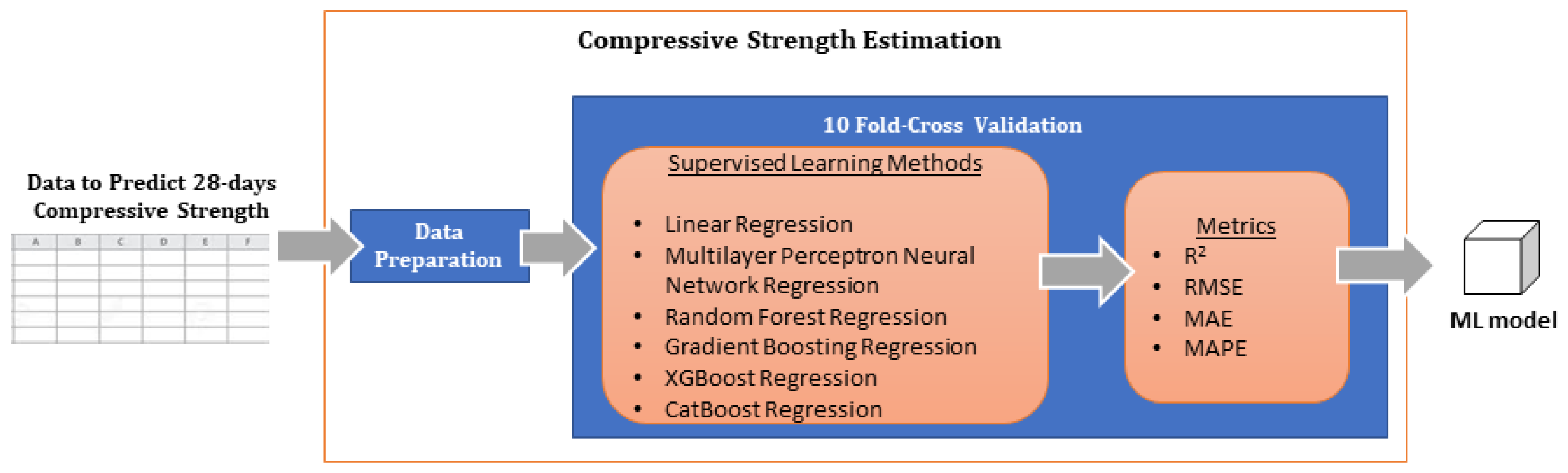
2.2.2. Compressive Strength Estimation

The compressive strength estimation, being a regression task, necessitates a historical dataset with compressive strength as the target variable, alongside predictor variables such as the free water; cement type; retarding admixture; superplasticizing admixture; SCM; fine aggregate source, quantity, and moisture; and coarse aggregate source, quantity, and moisture.

Table 3. Components of the dataset for training the $CS$ estimator.

Component	Units	Min	Max
Water	L/m3	40	200
Cement type I	kg/m3	200	1000
Cement type II	kg/m3	0	1000
Retarding admixture	g/m3	0	5000
Superplasticizing addmixture	g/m3	0	5000
SCM	kg/m3	0	100
Fine aggregate source	nominal
Fine aggregate quantity	kg/m3	0	2000
Fine aggregate moisture	%	0	15
Coarse aggregate source	nominal
Coarse aggregate quantity	kg/m3	0	2500
Coarse aggregate moisture	%	0	6
28th-day compressive strength (target variable)	MPa	10	100

describes the attributes of the dataset used for training the predictive model.

Different studies have been conducted to predict compressive strength with supervised learning methods, as summarized in [8,29], where most works barely reached a thousand samples. In a previous study [28], an architecture was designed to predict the compressive strength using a larger dataset, where the best-performing models used a multilayer perceptron neural network, gradient boosting, and random forest methods. The data from the previous study differ in that they considered concrete mixtures with fine aggregates from various sources, whereas the current study only includes concrete mixtures with fine aggregates from a single source. Following this approach, Figure 2 depicts the steps for building the machine learning model.

Dataset used for training: The estimator for the 28th-day $CS$ was trained on a dataset provided by the Colombian ready-mix company Cementos Argos S.A. (Medellín, Colombia). It should be noted that components such as the aggregates, specific materials, and chemical admixtures utilized in the preparation of the concrete may vary by geographical regions. However, the framework is general in the sense that the ML model can be easily retrained to tailor the specific materials and admixtures used in a particular context. This fine-tuning process can be easily automated to update the estimation models using new data due to changes in the admixtures, aggregates, or other components of the mixture.

Data preparation: The dataset provided for the assessment of the framework comprises approximately 19,000 mixture samples prepared and measured at Cementos Argos S.A. The presence of invalid samples was identified on an initial analysis of the data. These inconsistencies stem from errors during data collection, which may include human error, instruments miscalibrations, or failures at the data collection stage. Consequently, a data cleaning procedure was performed to eliminate outliers and samples with missing or invalid data. The cleaned dataset was then utilized for both training the ML algorithm to predict the $CS$ and for evaluating the solutions of the concrete mixture optimization framework. The data cleaning procedure involved the following steps:

• The removal of samples not meeting the volumetric restriction of 1 m³, thus resulting in the elimination of 4055 samples and leaving 15,239 samples in the dataset.
• The detection and removal of outliers using various outlier detection algorithms, including isolation forest trees, local outlier factor, and elliptic envelope. These are standard outlier detection algorithms included in thescikit-learn package [19]. After the outlier elimination step, 13,195 samples remained in the dataset.
• The verification of various restrictions on the remaining samples, such as water-to-cement ratio ranges and the ratios of fine aggregates to total aggregates. Samples failing to meet the restrictions were discarded, thus resulting in 11,428 definitive samples used for training and evaluating the optimization framework.
• The creation of dummy variables for nominal columns and the z normalization of numerical columns. The aggregate moisture and quantity variables were treated as different attributes for each of the sources. A correlation analysis was used to select the relevant variables.

Ten-fold crossvalidation: As ML estimators for predicting the quality attributes of the mixture, the following models were considered: the multilayer perceptron neural network, gradient boosting, and random forest methods (used in a previous work [28]), as well as the following additional models: linear regression, XGBoost, and Catboost. Crossvalidation was employed to evaluate the performance of the ML methods and to verify that there was not overfitting, thus generalizing on unseen data. This technique involves partitioning the dataset into multiple subsets or “folds”, with models tested on one of the folds and trained on the remainder. The error metrics employed during the crossvalidation included the coefficient of determination (R²), root mean square error (RMSE), mean absolute error (MAE), and mean percentage absolute error (MAPE).

2.2.3. Optimization of the Concrete Mixture

Considering the numerical nature of the estimators, a genetic algorithm (GA) was used for the solution approach to explore the decision variable space in the pursuit of optimal solutions. Figure 3 outlines the steps of the GA for optimizing the concrete mixture. The optimization takes as inputs requirements such as the target $CS$, type of fine and coarse aggregates, and material costs. The output is the vector X of the components of the mixture.

Genetic algorithms are a type of evolutionary algorithm that mimic natural selection to solve optimization problems [30]. The algorithm initiates by generating a random population of candidate solutions called individuals, each represented by a vector X—which in this case is the mixture vector shown in Figure 4—and then proceeds by performing the steps of parent selection, crossover, mutation, and survivor selection to produce a new offspring generation. This process is repeated over many generations, with the population of individuals gradually improving their fitness function.

The steps of the GA as implemented for the concrete optimization problem are as follows:

• Parent selection: During the selection process, each individual undergoes an evaluation of its fitness function $f_{GA}\left(X\right)$, and individuals with higher fitness have a higher probability of being selected for reproduction, while those with lower fitness have a lower probability.
• Crossover: This operation yields a new set of individuals by pairing parents $(X_i,X_j)$ and merging their genetic material—for instance, through a linear combination of the two vectors—to result in a new individual $X_k$.
• Mutation: This step introduces random alterations to some genes (vector components), thus aiming to enable mutated individuals to explore different regions of the solution space.
• Survivor selection: This step determines which individuals from the current population will pass on to the next generation. This process is based on the fitness of each individual, which is defined as a measure of its ability to solve the problem. The top-performing individuals are retained in the population (elitism).

Fitness function: The definition $f_{GA}\left(X\right)$ incorporates the cost function (5), quality constraints (2), and the volumetric constraint (3). The GA package manages range constraints (4), which are thus not included in the fitness function. Since the GA aims to minimize $f_{GA}$ (as per scipy’s implementation), the following considerations guide the construction of the fitness function:

• The cost function (1) yields values within the range $[0,\infty )$ in currency units, where cost minimization is the objective.
• The fractions within the quality constraints specified by (2) are dimensionless fractions within the range $[0,\infty )$, with 0 indicating perfect adherence to the constraint. These constraints include the target $CS$, the water–cement ratio, and the proportion of fine aggregates to the total aggregates.
• The volumetric constraint (3) represents the deviation from 1 m³. To penalize negative and positive deviations, the penalty is defined as the squared difference, which ensures that the error is in the range $[0,\infty )$.

In accordance with the previous considerations, the fitness function is defined as follows:

$$f_{GA}\left(X\right)=c\left(X\right)+\sum _i\frac{|f_{q_i}\left(X\right)-q_i|}{q_i}+{\left(\sum _j{x}_j·{\rho }_j-1\right)}^2$$

(5)

As the genetic algorithm progresses through iterations, the overall fitness gradually decreases over time, thereby approaching an asymptotic minimum until it either meets a minimum change criterion or exhausts the maximum number of generations. The solution returned is the fittest individual (minimizing $f_{GA}$) from the last generation.

2.2.4. Implementation and Deployment

The framework architecture was implemented using the Python (version 3.10) language. The compressive strength estimation used the scikit-learn, xgboost, and catboost packages to create the ML models. The optimization of the concrete mix cost was implemented using Python’s geneticalgorithm package for solving the optimization problem using a genetic algorithm. This library is designed to minimize the objective function for any number of independent variables, thus encompassing various types such as real, integer, and Boolean. It also manages range constraints for each decision variable while incorporating other constraints as penalty terms within the objective function, as detailed in the preceding section. The implemented optimization framework was deployed as a cloud service using Azure Cloud Functions. The algorithm runs as an asynchronous durable application, as typical execution periods span from 5 to 10 min. Subsequently, the algorithm determines the requisite quantities of coarse aggregate, fine aggregate, water, addmixtures (retarding and sustaining), and cement for the mix. Rigorous validation of the proposed concrete mix ensures the following: (1) compliance with the specified compressive strength, (2) the achievement of volumetric closure, and (3) adherence to concrete quality standards.

3. Results and Discussion

3.1. Compressive Strength Estimation

Table 4. Evaluation metrics for the considered regression techniques obtained using a 10-fold crossvalidation.

Regression Method	${\mathit{R}}^2$		RMSE (MPa)		MAE (MPa)		MAPE (%)
	Test	Train	Test	Train	Test	Train	Test	Train
CatBoost	0.76	0.88	5.32	3.90	4.10	3.00	10.52	7.79
RF	0.72	0.85	5.61	4.62	4.32	3.55	11.06	7.62
XGBoost	0.72	0.84	5.63	4.52	4.36	3.37	11.15	7.23
GBoost	0.71	0.81	5.64	4.85	4.38	3.73	11.35	9.74
MLP	0.71	0.82	5.71	4.36	4.34	3.29	11.32	8.51
Linear	0.68	0.89	6.12	5.16	5.12	3.93	12.32	10.16

shows the results of the evaluation metrics using the select ML algorithms. Compared with some of the results reported in the literature, there are cases with as little as 27 data points reporting an $R^2=0.80$ [10]. In Ref. [12] the authors reported predictions of the $CS$ using a dataset of 201 samples and reported an MAPE between $4.5\%$ and $13.5\%$. Similarly, in Ref. [9] the authors reported results with an MAPE between $\pm 10\%$ constructed with a dataset of 420 samples. Although not perfectly comparable because of the difference in the attributes in the datasets, the results of Table 4 show that these estimators performed similar or better with respect to various error metrics.

Across all the evaluation metrics, small disparities were observed between the errors in the training and test sets, thus indicating a strong potential for generalization to new data and a lack of overfitting. Overfitting happens when a machine learning model performs exceptionally well on the training data but struggles to make accurate predictions on new data, which was not the case in these experiments.

To evaluate if the performance of the machine learning methods differed significantly, an analysis of variance (ANOVA) was performed. The results indicated insufficient evidence to reject the null hypothesis, thus suggesting no significant differences among the methods. Similarly, the Tukey method confirmed these findings, thus showing no notable differences between each pair of methods. Remarkably, LR had weak performance in all metrics; therefore, it was discarded. With the aim of selecting one of the models, a comparison has been made using box plots. The MAPE measurements obtained from 10-fold crossvalidation were used to generate Figure 5, which enables the comparison of models using box plots, where a smaller spread implies greater consistency in the model’s performance.

Considering these findings, the CatBoost regression method was selected as the best $CS$ estimator model for the optimization framework. This decision was based on its superior performance across all error metrics on the test set and the smallest spread observed in the box plot. Figure 6 shows the plot of actual vs. predicted values for the compressive strength, as computed by the CatBoost algorithm. Also shown is the straight line representing the perfect fit between predictions and observations. In general, the predictions follow the ideal trend within some error margin. In this plot, it is also observed that the number of samples for large values of the $CS$ is quite reduced.

In order to detect outliers, a standardized residual graph is presented in Figure 7. A residual represents the difference between the actual and predicted values by a model. A standardized residual is a version of the residual that has been adjusted to have a mean of zero and a standard deviation of one, which is commonly used for detecting outliers. In the graph, points that significantly deviate from zero on the horizontal line can be considered outliers. Points that are well above zero may indicate that the model is underestimating the actual values. Conversely, points that are well below zero may indicate that the model is overestimating the actual values [31].

In the standardized residual graph (Figure 7), most points are distributed along the horizontal line at zero. This indicates that the model generally performed well without systematic bias. However, there are two outliers on the X axis, as well as six and nine on the Y axis of approximately 30 MPa. These outliers suggest instances where the model significantly underestimated the actual values, or they could be data errors, unusual values, or situations where the model did not adequately capture the underlying phenomenon.

Figure 8 depicts the distribution of the prediction errors of the model. It is observed that the model performed well with a high concentration of errors around zero. Two outliers are observed towards the right, which coincide with the two values found in the standardized residual plot. Although we are not aware of any standards regarding the magnitude of the error (either the absolute error, percentual error, or RMSE), there are standards for laboratory testing of concrete samples, such as the ASTM C39 [32], the ACI 318 [33], or the BS-8500 [34]. These standards call for preparing three samples of the mixture, thus measuring its compressive strength and verifying it is within a given tolerance percentage that is usually between 5% and 10% depending on the standard.

It is important to note that, although a dataset of over 10,000 observations may seem small compared to some machine learning studies, the quality and representativeness of the data are key aspects to consider. In machine learning studies for predicting concrete, datasets often contain a small number of records, sometimes fewer than 100, while a few may reach up to 1000 [29]. The literature review shows that most of these works have used datasets of sizes in the few hundreds. In this study, the data are real, they have been carefully collected by the company, and they represent a wide variety of relevant scenarios for the prediction problem. Additionally, data preprocessing and crossvalidation techniques were used to maximize the utility of the available data and mitigate the risk of overfitting. Future improvements of the predictive model would require more samples for large CS values.

Considering the particular nature of the dataset used in training the estimation framework, it may be argued that its generality is limited, since the model incorporates variables related to the source of the aggregates. In the case of changes in these variables, this necessitates retraining. Furthermore, the model must undergo regular updates and retraining with fresh data to accommodate temporal changes in the admixtures, cement properties, and aggregate quality in order to ensure sustained accuracy over time.

Despite the limitations in the predictive model, the proposed framework as a whole is robust with respect to its design and methodology, thus suggesting that when new datasets become available, retraining and fine-tuning would be sufficient to allow for their application under new circumstances. This characteristic also implies that the framework can potentially be used with other mixtures when given new training data. It is also noted that the model may experience variations over time—either by differences in the characteristics of the cement, aggregates, or admixtures used, as they may change over time. It can be argued that when performing a retraining process, the model can be fine-tuned to incorporate these changes, and this process can be incorporated as a function of the software for actual deployments. Given the proprietary nature of the data and intellectual property agreements between the involved organizations, further external validation and generalization studies would require collaboration with new partners and access to diverse datasets.

3.2. Optimization of Concrete Mixture Cost

Lacking prior knowledge regarding the optimality of samples in the dataset, the following procedure was adopted to assess the efficacy of the optimization framework:

• To construct a test case, a pair of coarse and fine aggregate sources was selected, and the dataset was filtered for these sources. Based on the resulting samples, a histogram of $CS$ was generated, and the interval with the highest sample count was identified. If the sample count fell below 10, the interval was discarded. This selection formed a set of samples, denoted as K, thus offering a representative sample size within a narrow $CS$ range for comparison against the solution of the optimization algorithm.
• The selected interval from step 1 represented the mode of samples for the chosen aggregate pair. The midpoint of this interval was designated as the target $CS$ for the optimization problem.
• The optimization algorithm was then executed to identify an optimal solution utilizing the same aggregates and the $CS$ determined in step 2. The optimization algorithm produced the optimized mixture, thus referred to as $X_{GA}$.
• It is noteworthy that $X_{GA}$ may not fully comply with all restrictions, as these are treated as penalties within the fitness function. Therefore, it was verified that the solution satisfied the restrictions.
• The cost of $X_{GA}$ was ranked along all samples in K in descending order of cost. A ranking of $100\%$ indicates that $X_{GA}$ has the lowest cost among all samples in K, while a ranking of $0\%$ signifies that $X_{GA}$ has the highest cost among the samples in K. This ranking served as an indicator of the optimality of solutions obtained by the optimization algorithm.
• The aforementioned procedure was repeated for N test cases utilizing different aggregate source combinations.

This assessment approach was implemented across $N=188$ instances. To gauge the quality of the obtained solutions, it was ensured that every instance that the $CS$ fell within the range of samples in the corresponding set K, thus validating that the predicted $CS$ was within the allowed percentage error.

To assess the cost efficiency of the solutions, the percentage of cases in the subset K with a higher cost than the $c\left(X_{GA}\right)$ was determined. In Figure 9, the y axis is the percentage of cases with a higher cost than the optimal found by the GA. A y value of $100\%$ indicates that the found solution has the lowest cost among all the samples in subset K. The x axis represents the percentage of test cases (out of 188). It is observed that for about $37\%$ of the cases, the GA found the best solution. The median of the distribution, denoted by a red dot, corresponds to half of test cases, for which the optimization framework obtained a solution with a cost lower than $98\%$ of test cases. In the far right of the graph, for $100\%$ of the test cases, the solution found by the framework had a lower cost than $60\%$ of the test cases in set K. These findings underscore that the framework’s solutions are generally cost-effective and meet the specified quality criteria.

3.3. Ethical Considerations

High errors in the prediction models could have impacts on the mix design quantities and mix performance. This is particularly important when predicting the compressive strength of concrete, as errors could be potentially related to structural failures depending on the concrete application. This work was developed with the goal of providing a tool for the RMX company’s quality assessment team to test and compare with the regular mix design process and not for the in-field formulation of mixtures and to determine how this new approach could mimic the process and support it. The purpose of the framework is to provide a first approximation in the design of new products and existing products, thus avoiding the need for long trial-and-error series of experiments and guaranteeing in all scenarios concrete mix performance.

Colombia has defined an ethical framework for artificial intelligence [35] with the aim of facilitating the implementation of the National Policy for Digital Transformation and Artificial Intelligence. Some of the key considerations in this framework are related to transparency, explainability, privacy, the human control of decisions, security, responsibility, nondiscrimination, inclusion, the prevalence of children’s and adolescents’ rights, and social benefit.

4. Conclusions

This study introduced a concrete mixture optimization framework that leverages ML estimators to calculate the properties of a given mixture and employs a genetic algorithm to identify optimal solutions. Within the framework, a singular optimization objective includes the cost function, quality attributes, and other constraints of the mixture stipulated by design considerations and industry standards. The framework subsequently identified mixtures that meet these specifications while minimizing the cost of the mixture. The following conclusions are drawn from this work:

• The framework effectively integrates machine learning and genetic algorithms to optimize concrete mixtures. It allows for cost optimization while maintaining specified compressive strength requirements and other mix design restrictions. The process ensures that the generated solutions are practical and meet user-defined constraints.
• Various machine learning models were evaluated to estimate compressive strength. The best prediction performance was obtained by the CatBoost regression algorithm, which achieved superior performance for all error metrics and consistency in its predictions. The model demonstrated strong generalization capabilities, with minimal disparities between the training and test set errors, thus indicating that it was not overfitted.
• The optimization algorithm was assessed by comparing its solutions against a representative set of samples. The optimization process was evaluated across 188 test cases considering different combinations of aggregates and the target compressive strength. The cost of the optimized mixture was compared with the real data points of similar characteristics. The comparison showed that approximately $37\%$ of the cases yielded the lowest cost solutions among the similar samples. The median of the optimized cost cases was more cost-effective than $98\%$ of the comparable samples.

To enhance model accuracy, future improvements should focus on expanding the dataset, particularly for higher compressive strength values. Deployments of the framework could benefit from continuous data collection, preprocessing, and retraining. Additionally, optimizing the genetic algorithm, exploring alternative fitness functions and penalty handling strategies, and investigating other optimization techniques may lead to more cost-effective solutions.

References

1. Mehta, P.K.; Monteiro, P.J.M. Concrete: Microstructure, Properties, and Materials, 4th ed.; McGraw Hill: New York, NY, USA, 2014. [Google Scholar]
2. Hover, K.C. The influence of water on the performance of concrete. Constr. Build. Mater. 2011, 25, 3003–3013. [Google Scholar] [CrossRef]
3. Kosmatka, S.H.; Panarese, W.C.; Kerkhoff, B. Design and Control of Concrete Mixtures; Portland Cement Association: Washington, DC, USA, 2005. [Google Scholar]
4. Mehta, P.K. Advancements in Concrete Technology. Concr. Int. 1999, 21, 69–76. [Google Scholar]
5. Crompton, S. Advances in Concrete Technology. Concr. Int. 2010, 21, 69–76. [Google Scholar]
6. DeRousseau, M.A.; Kasprzyk, J.R.; Srubar, W.V. Multi-objective optimization methods for designing low-carbon concrete mixtures. Front. Mater. 2021, 8, 680895. [Google Scholar] [CrossRef]
7. Park, W.; Noguchi, T.; Lee, H. Genetic algorithm in mix proportion design of recycled aggregate concrete. Comput. Concr. 2013, 11, 183–199. [Google Scholar] [CrossRef]
8. Nunez, I.; Marani, A.; Flah, M.; Nehdi, M.L. Estimating compressive strength of modern concrete mixtures using computational intelligence: A systematic review. Constr. Build. Mater. 2021, 310, 125279. [Google Scholar] [CrossRef]
9. Abbas, Y.M.; Khan, M.I. Robust machine learning framework for modeling the compressive strength of SFRC: Database Compilation, Predictive Analysis, and Empirical Verification. Materials 2023, 16, 7178. [Google Scholar] [CrossRef]
10. Ahmad, S.; Alghamdi, S.A. A statistical approach to optimizing concrete mixture design. Sci. World J. 2014, 2014, 561539. [Google Scholar] [CrossRef]
11. Kharazi, M. Designing and Optimizing of Concrete Mix Proportion Using Statistical Mixture Design Methodology. Master’s Thesis, Memorial University of Newfoundland, St. John’s, NL, Canada, 2013. [Google Scholar]
12. Parichatprecha, R.; Nimityongskul, P.; Parichatprecha, R.; Nimityongskul, P. An integrated approach for optimum design of HPC mix proportion using genetic algorithm and artificial neural networks. Comput. Concr. 2009, 6, 253. [Google Scholar] [CrossRef]
13. Amirjanov, A.; Sobol, K. Optimal proportioning of concrete aggregates using a self-adaptive genetic algorithm. Comput. Concr. 2005, 2, 411–421. [Google Scholar] [CrossRef]
14. DeRousseau, M.A.; Kasprzyk, J.R.; Srubar, W.V., III. Computational design optimization of concrete mixtures: A review. Cem. Concr. Res. 2018, 109, 42–53. [Google Scholar] [CrossRef]
15. Reed, P.M.; Hadka, D.; Herman, J.D.; Kasprzyk, J.R.; Kollat, J.B. Evolutionary multiobjective optimization in water resources: The past, present, and future. Adv. Water Resour. 2013, 51, 438–456. [Google Scholar] [CrossRef]
16. Zheng, W.; Shui, Z.; Xu, Z.; Gao, X.; Zhang, S. Multi-objective optimization of concrete mix design based on machine learning. J. Build. Eng. 2023, 76, 107396. [Google Scholar] [CrossRef]
17. Yang, S.; Chen, H.; Feng, Z.; Qin, Y.; Zhang, J.; Cao, Y.; Liu, Y. Intelligent multiobjective optimization for high-performance concrete mix proportion design: A hybrid machine learning approach. Eng. Appl. Artif. Intell. 2023, 126, 106868. [Google Scholar] [CrossRef]
18. Chen, F.; Xu, W.; Wen, Q.; Zhang, G.; Xu, L.; Fan, D.; Yu, R. Advancing concrete mix proportion through hybrid intelligence: A multi-objective optimization approach. Material 2023, 16, 6448. [Google Scholar] [CrossRef] [PubMed]
19. Virtanen, P.; Gommers, R.; Oliphant, T.E.; Haberland, M.; Reddy, T.; Cournapeau, D.; Van Mulbregt, P. SciPy 1.0: Fundamental algorithms for scientific computing in Python. Nat. Methods 2020, 17, 261–272. [Google Scholar] [CrossRef] [PubMed]
20. Zhang, J.; Huang, Y.; Wang, Y.; Ma, G. Multi-objective optimization of concrete mixture proportions using machine learning and metaheuristic algorithms. Constr. Build. Mater. 2020, 253, 119208. [Google Scholar] [CrossRef]
21. Song, Y.; Wang, X.; Li, H.; He, Y.; Zhang, Z.; Huang, J. Mixture Optimization of Cementitious Materials Using Machine Learning and Metaheuristic Algorithms: State of the Art and Future Prospects. Material 2022, 15, 7830. [Google Scholar] [CrossRef]
22. Charhate, S.; Subhedar, M.; Adsul, N. Prediction of Concrete Properties Using Multiple Linear Regression and Artificial Neural Network. J. Soft Comput. Civ. Eng. 2018, 2, 27–38. [Google Scholar] [CrossRef]
23. Grajski, K.A.; Breiman, L.; Prisco, G.V.D.; Freeman, W.J. Classification of EEG Spatial Patterns with a Tree-Structured Methodology: CART. IEEE Trans. Biomed. Eng. 1986, BME-33, 1076–1086. [Google Scholar] [CrossRef]
24. Gholami, R.; Fakhari, N. Support Vector Machine: Principles, Parameters, and Applications; Academic Press: Cambridge, MA, USA, 2017; pp. 515–535. [Google Scholar] [CrossRef]
25. Li, H.; Lin, J.; Lei, X.; Wei, T. Compressive strength prediction of basalt fiber reinforced concrete via random forest algorithm. Mater. Today Commun. 2022, 30, 103117. [Google Scholar] [CrossRef]
26. Alhakeem, Z.M.; Jebur, Y.M.; Henedy, S.N.; Imran, H.; Bernardo, L.F.; Hussein, H.M. Prediction of Ecofriendly Concrete Compressive Strength Using Gradient Boosting Regression Tree Combined with GridSearchCV Hyperparameter-Optimization Techniques. Material 2022, 15, 7432. [Google Scholar] [CrossRef] [PubMed]
27. Wu, Y.; Huang, H. Predicting compressive and flexural strength of high-performance concrete using a dynamic Catboost Regression model combined with individual and ensemble optimization techniques. Mater. Today Commun. 2024, 38, 108174. [Google Scholar] [CrossRef]
28. Vargas, J.F.; Oviedo, A.I.; Ortega, N.A.; Orozco, E.; Gómez, A.; Londoño, J.M. Machine-Learning-Based Predictive Models for Compressive Strength, Flexural Strength, and Slump of Concrete. Appl. Sci. 2024, 14, 4426. [Google Scholar] [CrossRef]
29. Li, D.; Tang, Z.; Kang, Q.; Zhang, X.; Li, Y. Machine Learning-Based Method for Predicting Compressive Strength of Concrete. Processes 2023, 11, 390. [Google Scholar] [CrossRef]
30. Holland, J.H. Adaptation in Natural and Artificial Systems; University of Michigan Press: Ann Arbor, MI, USA, 1975. [Google Scholar]
31. Suleiman, A.; Abdullahi, U.; Ahmad, U.A. An Analysis of Residuals in Multiple Regressions. Int. J. Adv. Sci. Eng. 2015, 3, 2348–7550. [Google Scholar]
32. C39/C39M; Standard Test Method for Compressive Strength of Cylindrical Concrete Specimens. American Society for Testing and Materials (ASTM): West Conshohocken, PA, USA, 2017.
33. ACI CODE-318-19(22); Building Code Requirements for Structural Concrete and Commentary (Reapproved 2022). American Concrete Institute (ACI): Columbia, MD, USA, 2014.
34. BS 8500-1:2023; BSI Knowledge. British Standards Institution (BSI): London, UK, 2023.
35. Marco ético Para la Inteligencia Artificial en Colombia; Technical Report; Gobierno de Colombia: Bogotá, Colombia, 2021.
Figure 1. Overall architecture of the optimization framework.
Modelling 05 00034 g001
Figure 2. C S estimator based on an ML model.
Modelling 05 00034 g002
Figure 3. GA for optimizing the concrete mixture.
Modelling 05 00034 g003
Figure 4. Vector representing “individuals” in the GA.
Modelling 05 00034 g004
Figure 5. Performance comparison using test data.
Modelling 05 00034 g005
Figure 6. Actual vs. predicted values for C S . Blue crosses are the predictions, red line represents a perfect prediction.
Modelling 05 00034 g006
Figure 7. Standardized residuals of predicted vs. actual values of C S . Blue dots are the residuals of the predictions, the red line is the zero residual line.
Modelling 05 00034 g007
Figure 8. Distribution of prediction errors.
Modelling 05 00034 g008
Figure 9. Percentage of cases where optimized solution has a lower cost. Blue line is the percentage of cases with higher cost than the solution of the optimization. The red dot indicates the median percentage across all test cases.
Modelling 05 00034 g009