Micromechanical Estimates Compared to FE-Based Methods for Modelling the Behaviour of Micro-Cracked Viscoelastic Materials

Abstract

The purpose of this study is to investigate the effective behaviour of a micro-cracked material whose matrix bulk and shear moduli are ruled by a linear viscoelastic Burgers model. The analysis includes a detailed study of randomly oriented and distributed cracks displaying an overall isotropic behaviour, as well as aligned cracks resulting in a transversely isotropic medium. Effective material properties are approximated with the assumption that the homogenized equivalent medium exhibits the characteristics of a Burgers model, leading to the identification of short-term and long-term homogenized modules in the Laplace–Carson space through simplified formulations. The crucial advantage of this analytical technique consists in avoiding calculations of the inverse Laplace–Carson transform. The micromechanical estimates are validated through comparisons with FE numerical simulations on 3D microstructures generated with zero-thickness void cracks of disc shape. Intersections between randomly oriented cracks are accounted for, thereby highlighting a potential percolation phenomenon. The effects of micro-cracks on the material’s behaviour are then studied with the aim of providing high-performance creep models for macrostructure calculations at a moderate computation cost through the application of analytical homogenization techniques.

1. Introduction

In the context of long-term deep disposal of nuclear waste in the Callovo-Oxfordian (COx) claystone, the excavation of tunnels in the host rock inevitably leads to macroscopic fracturing, raising potentially significant challenges for nuclear waste management [1,2,3]. Characterizing the behaviour of the COx claystone is complex, as various factors are involved in determining the appropriate behaviour of the claystone. In particular, the creep properties of the argillite play a crucial role in the crack sealing process [4], an anticipated key phase expected to take place following the closure of the underground waste disposal [5]. This study aims to provide a description for the creep phenomenon within a simplified linear viscoelastic framework. Furthermore, it is intended to model the behaviour of a fractured viscoelastic material by approximating its effective properties and identifying the parameters by means of a macroscopic Burgers model [6]. For the purpose of validating the analytical approach, the results are compared with numerical simulations performed using the finite element method with the Cast3M (http://www-cast3m.cea.fr/ (version 2022, accessed on 4 April 2022)) software. This comparison between the two approaches offers key validation requirements when it comes to modelling the macroscopic behaviour of damaged materials while exploiting the use of multi-scale approaches. The excavation of tunnels for the Cigéo project causes fracturing of the COx claystone. Characterizing the cracking state through in situ observations provides means for dimensioning the damaged zone and determining crack orientations as a function of distance from the excavated drifts. In the vicinity of the galleries, crack orientations appear widely variable and random. With increasing distance from the drifts, cracks show preferential orientations mostly parallel to the galleries [2].

Several techniques are employed to accurately describe the complex phenomenon of fracture in materials [7,8,9,10,11]. Alongside damage models, which incorporate the effect of cracks by introducing a damage variable [12], methods based on continuum mechanics can also capture the presence of cracking in a solid material [13]. In particular, micromechanical techniques based on the calculation of homogenized moduli can be used to estimate the effect of fractures on the material’s macroscopic properties [14,15,16]. Cracks are considered as heterogeneities distributed in the solid matrix, and solutions based on micromechanical estimates are presented to deduce homogenized properties. The approach used by Budiansky and O’connell [17] involves the utilization of a crack density parameter to characterize the fracturing effect, assuming that all cracks are circular with an identical shape and size. The crack density parameter can be associated macroscopically with a damage variable, whose effects are calculated from analytical homogenization schemes [18]. In addition, other techniques, notably finite element modelling [19], can be used to create microstructures representative of the fracturing condition, with considerably fewer limitations in terms of design simplifications. This numerical approach can be directly compared to analytical techniques obtained by approximation schemes, which is a key objective of this study.

Materials subjected to constant loads can exhibit a delayed (creep) behaviour, characterized by continuous deformation over time. Linear viscoelastic models can depict such effects in a simplified context [20]. Moreover, it is possible to use the Laplace–Carson transform (LC) and proceed to operate with an equivalent linear elastic behaviour in the Laplace–Carson space. This provides a straightforward framework to have recourse to for analytical solutions obtained with classical homogenization procedures developed for elastic materials affected by the presence of cracks and/or heterogeneities [21]. For this purpose, the behaviour of the COx claystone is represented here by non-ageing linear viscoelastic Burgers models combining Maxwell and Kelvin–Voigt models. Using a minimum number of parameters, the Burgers model is indeed able to capture the main features of a viscoelastic material behaviour, particularly providing an adequate representation of the long-term characteristics of the COx claystone. In linear viscoelastic applications, dealing with heterogeneous media considerably complexifies the formulated equations in LC space. This difficulty renders model equation inversion into real time space challenging. Commonly, numerical solutions, such as the collocation method, are used to provide effective resolutions to the equations describing the material’s behaviour [22,23].

Most classical approaches used to estimate the behaviour of heterogeneous materials with homogenization techniques are based on the Eshelby solution [24]. These approaches have proved to be very efficient for approximating the effective behaviour of such materials in various contexts, including for micro-cracked linear elastic materials [19,25]. In this case, an alternative approach has been proposed in [26], based on the linear relationship between macroscopic stress and the discontinuity of local displacements across the crack. This approach will be explored in the present study, together with an approximation method assuming that the effective behaviour of the material can be represented by a set of Burgers models. This efficient method provides an analytical solution of the model equations in simplified forms, making inversion calculations analytically achievable. One key advantage is that their parameters can be directly expressed as a function of the parameters of the viscoelastic models describing the sound material and the crack density parameter characterizing the cracking state. This differs from more classical approaches based on the application of homogenization schemes in the LC space, which generally requires a numerical inversion to characterize the model in the time space. The analytical results will be compared to finite element simulations obtained using 3D samples generated with disc-shaped voids of zero thickness, thus mimicking very accurately the behaviour of micro-cracked materials. In this context, the material’s behaviour will be analysed by considering relevant cases of crack orientations including randomly oriented cracks as well as a parallel crack distribution in an isotropic medium.

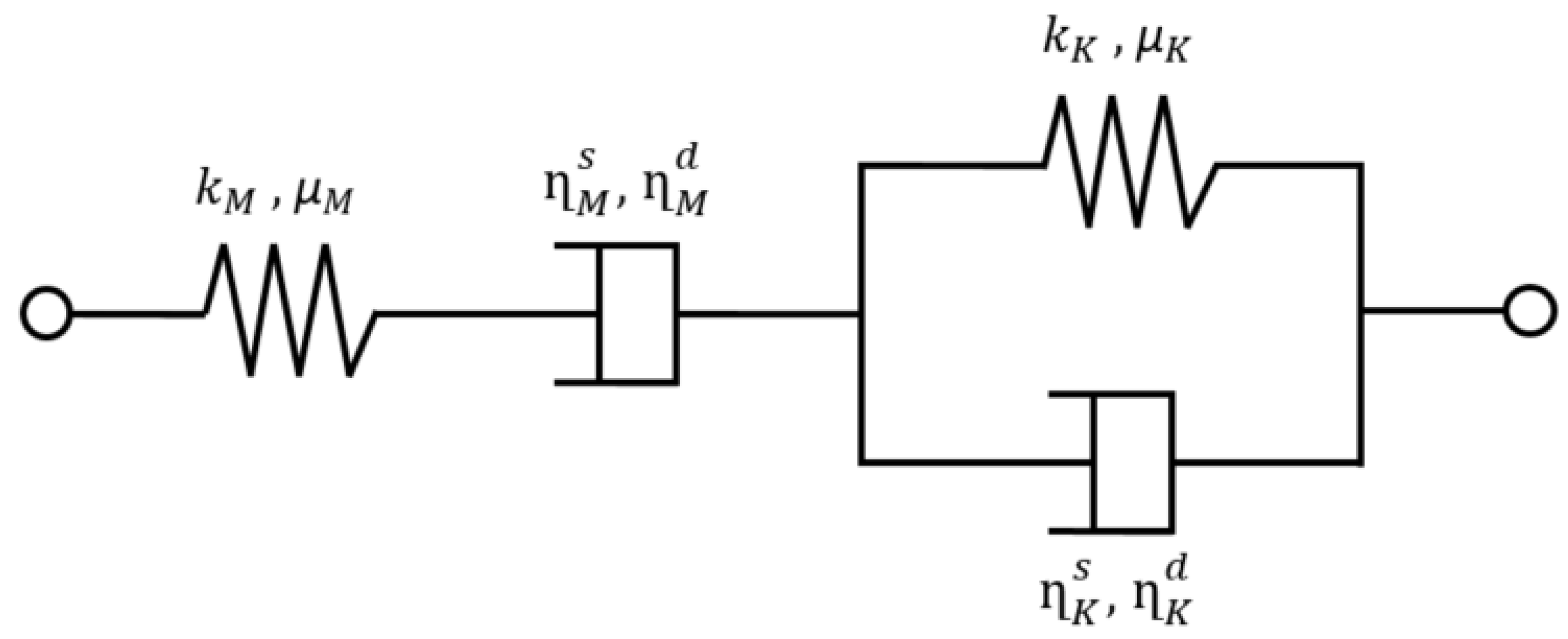
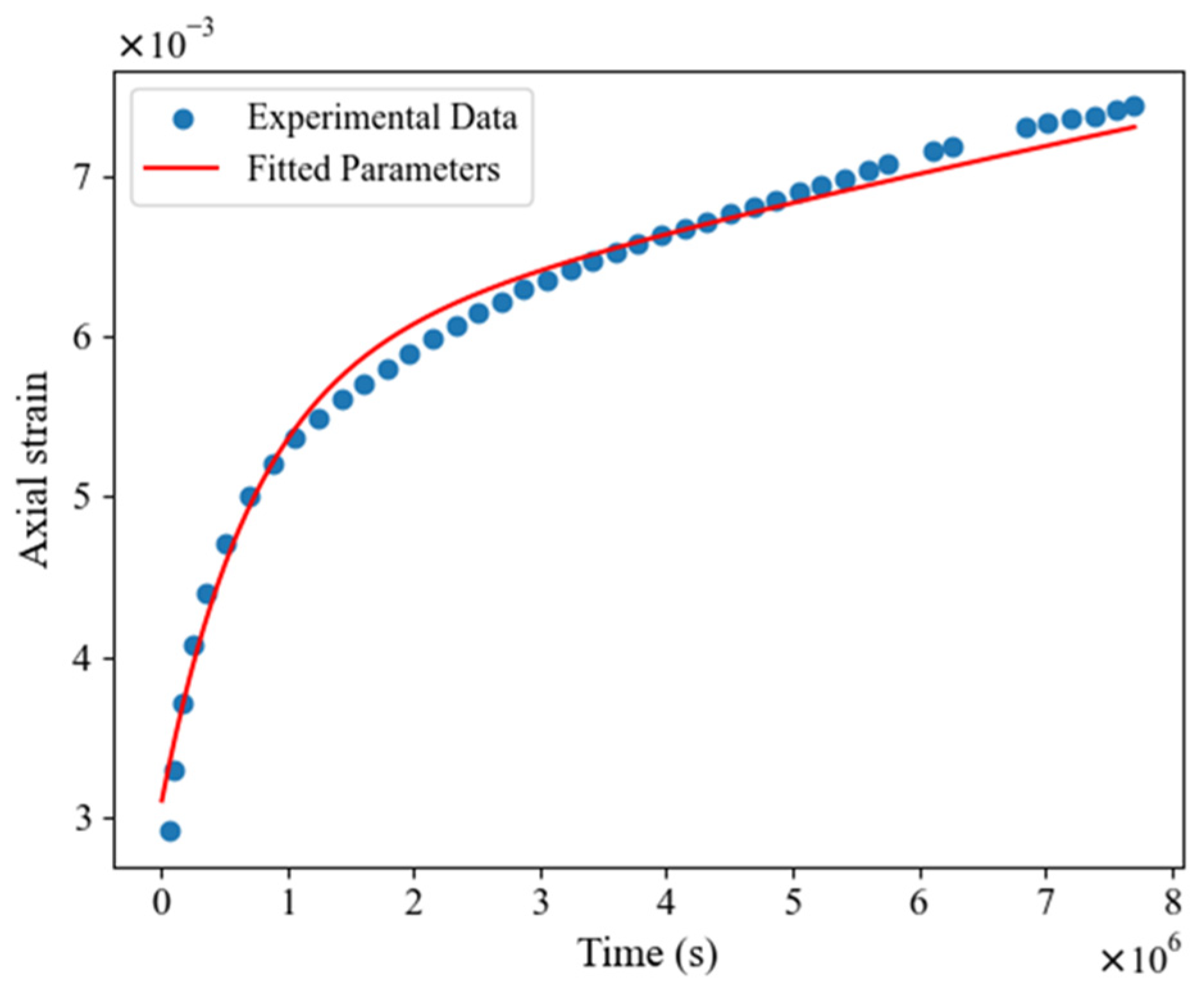
2. Viscoelastic Burgers Model

The majority of bedrock masses, when subjected to a permanent stress, exhibit to some degree a deferred behaviour, which is expressed by an increase in strain under constant loading. This phenomenon indicates that a complete description of the constitutive behaviour of a rock mass must assume time-dependence. A rigorous approach is to use viscoelastic or viscoplastic behaviour laws to describe the evolution of the creep phenomenon for geomaterials [4,27,28]. In analysing the behaviour of the Callovo-Oxfordian claystone, the effect of delayed long-term response of the material must be taken into account to ensure an accurate representation of the COx claystone [29]. In this context, we focus mainly on non-ageing linear viscoelastic models, which allow establishing a linear relation between the stress and strain in the Laplace–Carson space using the correspondence principle. The development of the Burgers model equations provides an efficient representation of the material’s short- and long-term behaviour, while requiring a limited number of parameters. It is intended to use this model to represent the behaviour of the COx claystone. The indices M and K designate, respectively, the Maxwell and Kelvin parts of the model, while exponents s and d are attributed to the spherical and deviatoric parts of the model (Figure 1). Moreover, we propose to use two different Burgers models to describe independently the shear and bulk moduli denoted by μ and k, respectively.

$$\frac{1}{k^{*}}=\frac{1}{k_M}+\frac{1}{p\frac{{\mathsf{\eta }}_M^s}{3}}+\frac{1}{k_K+p\frac{{\mathsf{\eta }}_K^s}{3}};\frac{1}{{\mathsf{\mu }}^{*}}=\frac{1}{{\mathsf{\mu }}_M}+\frac{1}{p\frac{{\mathsf{\eta }}_M^d}{2}}+\frac{1}{{\mathsf{\mu }}_K+p\frac{{\mathsf{\eta }}_K^d}{2}}$$

(1)

Equation (1) expresses the effective compressibility and shear moduli in Laplace–Carson space, denoted by $k^{*}$ and ${\mu }^{*}$, respectively, where p is the LC variable. The eight parameters of the Burgers model can be distinguished in Equation (1). The Maxwell part is represented by four parameters, including spherical components ($k_M,{\mathsf{\eta }}_M^s$) and deviatoric components (${\mathsf{\mu }}_M,{\mathsf{\eta }}_M^d$). Additionally, the Kelvin part of the model is also composed of four parameters, with ($k_K,{\mathsf{\eta }}_K^s$) describing the spherical parameters and (${\mathsf{\mu }}_K,{\mathsf{\eta }}_K^d$) representing the deviatoric components. The parameters of the Burgers models are identified through an analytical resolution of the strain under constant stress loading, followed by comparisons with experimental creep testing results. Armand et al. [30] have published a series of creep tests widely used in the literature to characterize this phenomenon. Cores of COx were extracted from the Meuse/Haute-Marne underground research laboratory, and the samples were drilled perpendicular to the bedding plane of the rock, as the COx claystone naturally exhibits a transversely isotropic behaviour. These tests include different series of loadings and have been designed to examine the deferred behaviour of the material for different loading conditions. The applied loadings are a function of the maximum deviatoric stress that the material can withstand. The argillite is considered anisotropic, and therefore, its properties change as a function of the imposed loading with respect to the bedding plane. Here, for conformity, the solid material will be considered isotropic, meaning that the elastic moduli do not vary with respect to the bedding plane. The model parameters have been identified under loading conditions corresponding to 75% of the maximum deviatoric stress.

The use of numerical models with a number of parameters can render the precise identification of each parameter from a single experimental test complex. Although some simplifications can be achieved at the limits as time tends to zero or infinity, it remains difficult to identify each parameter individually. Consequently, optimization methods were employed to refine the model parameters. The least-squares method is used to optimize the Burgers model parameters using standard Python libraries (Figure 2). The normal and tangential components of the strain tensor (${\mathsf{\epsilon }}_{nn}$ and ${\mathsf{\epsilon }}_{tt}$, respectively) in the time space are identified by calculating the inverse of the Carson–Laplace transform of:

$${\mathsf{\epsilon }}^{*}=\frac{1+{\nu }^{*}}{E^{*}}{\mathsf{\sigma }}^{*}-\frac{{\nu }^{*}}{E^{*}}tr\left({\mathsf{\sigma }}^{*}\right)\mathit{I}$$

(2)

where the superscript * stands for a quantity expressed in the LC space. The normal and tangential strain components due to the application of a uniaxial constant stress ${\sigma }_0$ can be deduced in LC space from Equation (2):

$${\mathsf{\epsilon }}_{nn}^{*}=\frac{{\sigma }_0}{E^{*}} and {\mathsf{\epsilon }}_{tt}^{*}=\frac{-{\sigma }_0{\nu }^{*}}{E^{*}}$$

(3)

Inversion of the normal strain ${\mathsf{\epsilon }}_{nn}^{*}$ from LC space yields:

$$\begin{gathered} {\mathsf{\epsilon }}_{nn}=\frac{{\sigma }_0}{E_M}+\frac{{\sigma }_0}{9k_M}\frac{t}{\left(\frac{{\mathsf{\eta }}_M^s}{3k_M}\right)}+\frac{{\sigma }_0}{3{\mu }_M}\frac{t}{\left(\frac{{\mathsf{\eta }}_M^d}{2{\mu }_M} \right)}+\frac{{\sigma }_0}{9k_K}\left(1-e^{-\frac{t}{\frac{{\mathsf{\eta }}_K^s}{3k_K}}}\right)+\frac{{\sigma }_0}{3{\mu }_k}\left(1-e^{-\frac{t}{\frac{{\mathsf{\eta }}_K^d}{2{\mu }_K}}}\right) \\ \mathrm{with} {\nu }_M=\frac{3k_M-2{\mu }_M}{6k_M+2{\mu }_M} \mathrm{and} \frac{1}{E_M}=\frac{1}{9k_M}+\frac{1}{3{\mu }_M} \end{gathered}$$

(4)

This expression involves the eight parameters of the Burgers model and the time.

Overall, the proposed model provides an acceptable representation of the argillite’s behaviour in both the short and long term, see Figure 2 for the comparison between experimental and numerical results of a creep test. The characteristic parameters of the Burgers model are summarized in

Table 1. Identified viscoelastic parameters of the COx claystone.

Parts	$\mathit{k} \left(\mathbf{G}\mathbf{P}\mathbf{a}\right)$	$\mathsf{\mu } \left(\mathbf{G}\mathbf{P}\mathbf{a}\right)$	${\mathsf{\eta }}^{\mathit{s}} \left(\mathbf{G}\mathbf{P}\mathbf{a}.\mathbf{s}\right)$	${\mathsf{\eta }}^{\mathit{d}} \left(\mathbf{G}\mathbf{P}\mathbf{a}.\mathbf{s}\right)$
Maxwell	6.872	3.870	$35.381·{10}^7$	$12.463·{10}^7$
Kelvin	7.308	3.099	$26.364·{10}^6$	$4.020·{10}^6$

.

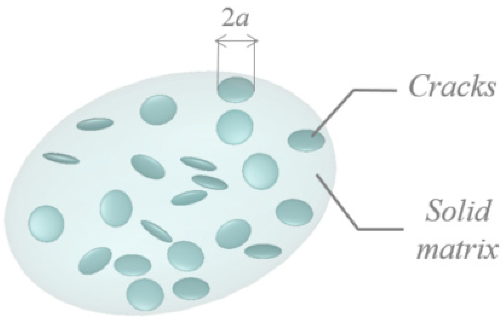
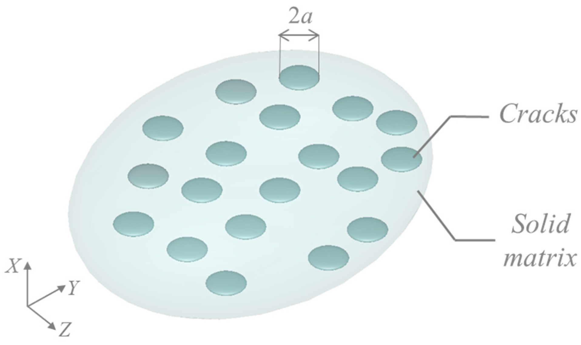
3. Representation of Cracking in a Viscoelastic Material

In this work, we make use of the approach proposed in [6,26,31,32] for considering the presence of cracks, which is not directly based on Eshelby’s classical approach [24], although is very close. The interested reader is invited to refer to the cited papers for more details that would be too lengthy to include here.

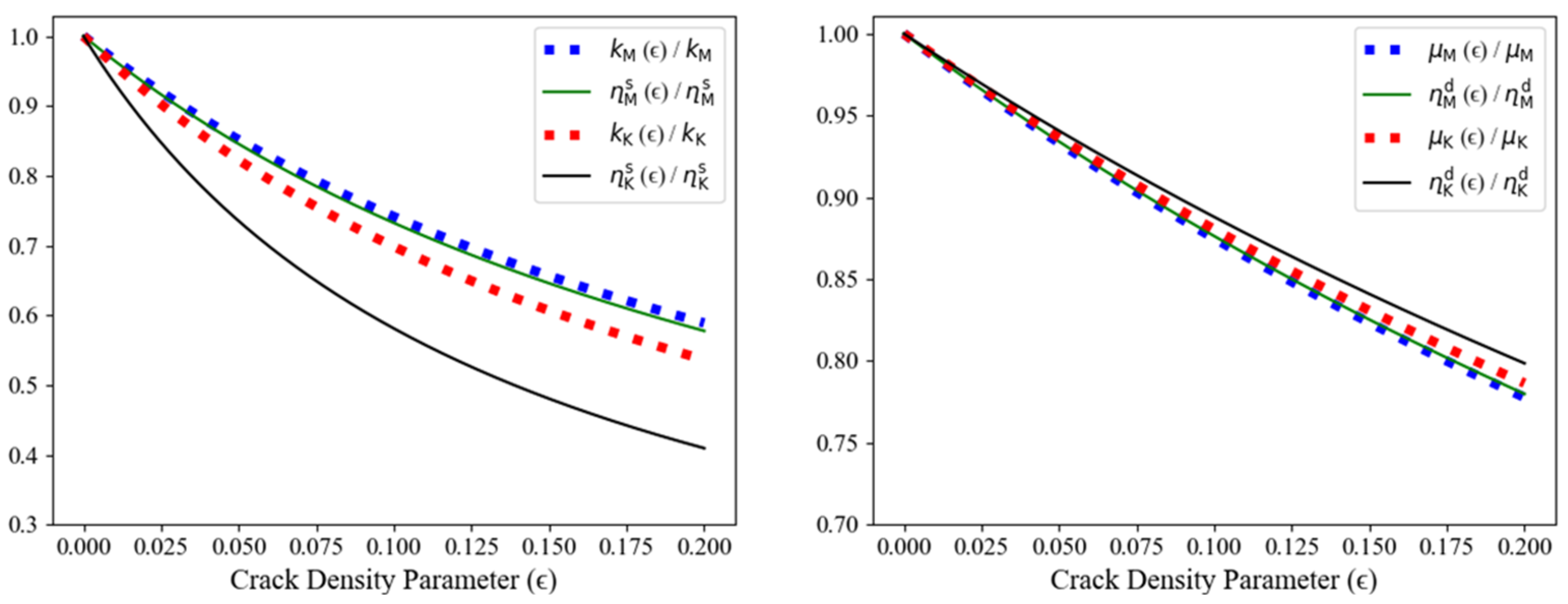
3.1. Isotropic Crack Distribution

Considering an isotropic distribution of cracks in a solid matrix (Figure 3), where cracks are characterized by the crack density parameter $ϵ$ in which N is the number of cracks per unit volume of REV (Representative Elementary Volume) and a is the crack radius, assuming an identical circular shape and a uniform size for all cracks (Equation (5)).

$$ϵ=N{a}^3$$

(5)

The apparent effective stiffness tensor in the Laplace–Carson space defined by ${ℂ}^{ho{m}^{*}}$ is therefore isotropic, expressed in the ($\mathbb{J}$,$\mathbb{K}$) basis in Equation (6). The tensors $\mathbb{J}$ and $\mathbb{K}$ are, respectively, the projectors of the spherical and deviatoric parts of the fourth-order unit tensor.

$${ℂ}^{ho{m}^{*}}=3k^{ho{m}^{*}}\mathbb{J}+2{\mu }^{ho{m}^{*}}\mathbb{K}$$

(6)

The homogenized moduli $k^{ho{m}^{*}}$ and ${\mathsf{\mu }}^{ho{m}^{*}}$ are calculated as a function of the crack density parameter $ϵ$, taking into account two distinct loading conditions: spherical loading, which is used to determine the compressibility modulus, and deviatoric loading, which is used to determine the shear modulus. A homogenized stiffness matrix is then constructed in the LC space, reflecting the material cracking conditions [26].

$$\frac{1}{k^{ho{m}^{*}}}=\frac{1}{k^{*}}+\frac{8ϵ}{3} \frac{\left(1-{\nu }^{*}\right)}{{\mathsf{\mu }}^{*}}$$

(7)

$$\frac{1}{{\mathsf{\mu }}^{ho{m}^{*}}}=\frac{1}{{\mathsf{\mu }}^{*}}+\frac{32ϵ}{{\mathsf{\mu }}^{*}} \frac{\left(1-{\nu }^{*}\right)\left(5-{\nu }^{*}\right)}{45\left(2-{\nu }^{*}\right)}$$

(8)

To simplify, here, the homogenized material behaviour in the LC space is studied by considering a general analogy with a homogenized macroscopic Burgers model, i.e., we assume that the behaviour of the homogenized material can be approached by Burgers models. This makes it possible to identify the homogenized modules $k^{ho{m}^{*}}$ and ${\mathsf{\mu }}^{ho{m}^{*}}$ in the LC space using a simplified form:

$$\frac{1}{k^{ho{m}^{*}}}=\frac{1}{k_M\left(ϵ\right)}+\frac{1}{p{\mathsf{\eta }}_M^s\left(ϵ\right)/3}+\frac{1}{k_K\left(ϵ\right)+p{\mathsf{\eta }}_K^s\left(ϵ\right)/3}$$

(9)

$$\frac{1}{{\mathsf{\mu }}^{ho{m}^{*}}}=\frac{1}{{\mathsf{\mu }}_M\left(ϵ\right)}+\frac{1}{p{\mathsf{\eta }}_M^d\left(ϵ\right)/2}+\frac{1}{{\mathsf{\mu }}_K\left(ϵ\right)+p{\mathsf{\eta }}_K^d\left(ϵ\right)/2}$$

(10)

This maintains the same structure of the Burgers model formulated in Equation (1). Proceeding with a Taylor expansion of the expressions of the moduli with respect to the variable p in the Carson space in the vicinity of 0 and infinity, the eight parameters of the Burgers models can be identified as a function of the crack density parameter (Figure 4). A correlation of the parameters as a function of crack density (Equation (5)) is established, as illustrated in Figure 4. In summary, this approach provides an alternative method for characterizing the behaviour of a micro-cracked material in the Laplace–Carson space [6].

Determining the parameter equations as a function of crack density for a macroscopically cracked material of the Burgers type enables a straightforward formulation of the homogenized moduli that define this problem. This approach can provide an explicit formulation of the effective Burgers model equations in the time space as a function of the parameters of the undisturbed material and the crack density parameter (Equations (9) and (10)). This significantly reduces the complexity of the calculation of the modules in the time space as it avoids the direct application of the inverse of the Laplace–Carson transform on such equations. This in turn leads to the development of straightforward analytical solutions, offering results comparable to those obtained by alternative numerical approaches such as the finite element method [19] or the FFT approach, which also enable an analysis of the effective moduli on microstructures [7,33].

3.2. Parallel Crack Distribution

In this section, the effect of a random distribution of parallel cracks in a linear viscoelastic material, as described in the previous sections, will be discussed. In this case, a transversely isotropic behaviour is obtained (Figure 5). In this context, it is convenient to work with the expression of the material compliance tensor in LC space ${\mathbb{S}}^{*}\left(p\right)$ (Equation (11)), which is the inverse of the stiffness tensor using the Walpole basis [34]. Using the Walpole basis simplifies the expression of the viscoelastic compliance tensor in the case of anisotropy, making the analysis of modules affected by the fracturing more convenient.

$${\mathbb{S}}^{*}\left(p\right)={\displaystyle \sum }_{i=1}^6{s}_i^{*}\left(p\right){\mathbb{E}}_i$$

(11)

with

$$\begin{gathered} s_1^{*}\left(p\right)=\frac{1+{\nu }^{*}}{2{\mathsf{\mu }}^{*}\left(1+{\nu }^{*}\right)} ;s_2^{*}\left(p\right)=\frac{1}{2{\mathsf{\mu }}^{*}\left(1+{\nu }^{*}\right)} ;s_3^{*}\left(p\right)=\frac{1}{2{\mathsf{\mu }}^{*}} \\ {s}_4^{*}\left(p\right)=\frac{1}{2{\mathsf{\mu }}^{*}} ; s_5^{*}\left(p\right)=s_6^{*}\left(p\right)=-\frac{{\nu }^{*}}{2{\mathsf{\mu }}^{*}\left(1+{\nu }^{*}\right)} \end{gathered}$$

(12)

By decomposing the compliance tensor in the Walpole basis (Equation (11)), we obtain six scalars with indices i ranging from 1 to 6 denoted $s_i^{*}\left(p\right)$. The tensors ${\mathbb{E}}_i$ are defined in accordance with the specifications given in the Walpole basis [34]. Equation (12) describes the expressions of the scalars $s_i^{*}\left(p\right)$ in the Laplace–Carson space. Note that the directions $({\mathit{e}}_{\mathbf{1}}, {\mathit{e}}_{\mathbf{2}},{\mathit{e}}_{\mathbf{3}})$, respectively, correspond to the conventional directions in a Cartesian coordinate system (x, y, z). n is the direction normal to the fractures along ${\mathit{e}}_{\mathbf{1}}$ (Figure 5).

As demonstrated, e.g., in [26], the calculations highlight that for a transversely isotropic medium, some of the modules are not influenced by the cracking state of the material. This observation has been confirmed in an analysis of a linear elastic behaviour case, where only the Young’s modulus perpendicular to the bedding plane and the shear coefficients were affected by the cracking [35]. Following the notation for the scalar indices in the Walpole’s basis, the expression for the moduli $s_2^{ho{m}^{*}}$ and $s_4^{ho{m}^{*}}$ as a function of the cracking density yields:

$$s_2^{ho{m}^{*}}=s_{M2}^e\left(ϵ\right)+\frac{1}{p}{s}_{M2}^v\left(ϵ\right)+{\left(s_{K2}^e{\left(ϵ\right)}^{-1}+p{s}_{K2}^v{\left(ϵ\right)}^{-1}\right)}^{-1}$$

(13)

$$s_4^{ho{m}^{*}}=s_{M4}^e\left(ϵ\right)+\frac{1}{p}{s}_{M4}^v\left(ϵ\right)+{\left(s_{K4}^e{\left(ϵ\right)}^{-1}+p{s}_{K4}^v{\left(ϵ\right)}^{-1}\right)}^{-1}$$

(14)

provided that $s_2^{ho{m}^{*}}$ and $s_4^{ho{m}^{*}}$ are the two moduli affected by the cracking [26]. The exponents e and v are attributed to the elastic and viscous parts, respectively. The model parameters are determined based on the assumption that the macroscopic model is essentially of the Burgers type, allowing the parameters to be identified with simplified analytical expressions, analogous to the isotropic case discussed in the previous section. The determination of $s_2^{ho{m}^{*}}$ is obtained by imposing a uniaxial tensile load along the normal to the cracks, while that of $s_4^{ho{m}^{*}}$ requires a shear loading in the form $\sigma \left({\mathit{e}}_{\mathbf{2}}\otimes \mathit{n}+\mathit{n}\otimes {\mathit{e}}_{\mathbf{2}}\right)$, e.g., with $\sigma =1 \mathrm{MPa}$. As the other modules will not be affected by the cracks, it is possible to attribute to them the modules of the undisturbed material without requiring further calculations.

The same identification technique as for the isotropic case was used, considering that the homogenized behaviour of the cracked material corresponds to a macroscopic Burgers model, while accounting for the crack density parameter. Conserving the same structure of the Burgers model formulation, it is possible to define a correlation of the eight coefficients in Equations (13) and (14) as a function of crack density (Equation (5)), as shown in Figure 6. The moduli affected by cracking in a Cartesian coordinate system, such as $E_1^{hom}$ and ${\mu }_{12}^{hom}$, can be determined from calculations in the Walpole basis as a function of the coefficients $s_2^{hom}$ and $s_4^{hom}$ [34]. As mentioned above, investigating the transversely isotropic case is representative of the in situ behaviour of the fractured COx claystone, since in reality, fracture formation in parts of the damaged zone is produced with a preferential orientation parallel to the excavated drifts [2]. A more in-depth analysis of the analytical results is carried out by comparing the results with the numerical simulations obtained with the Cast3M finite element code.

4. Numerical Simulations

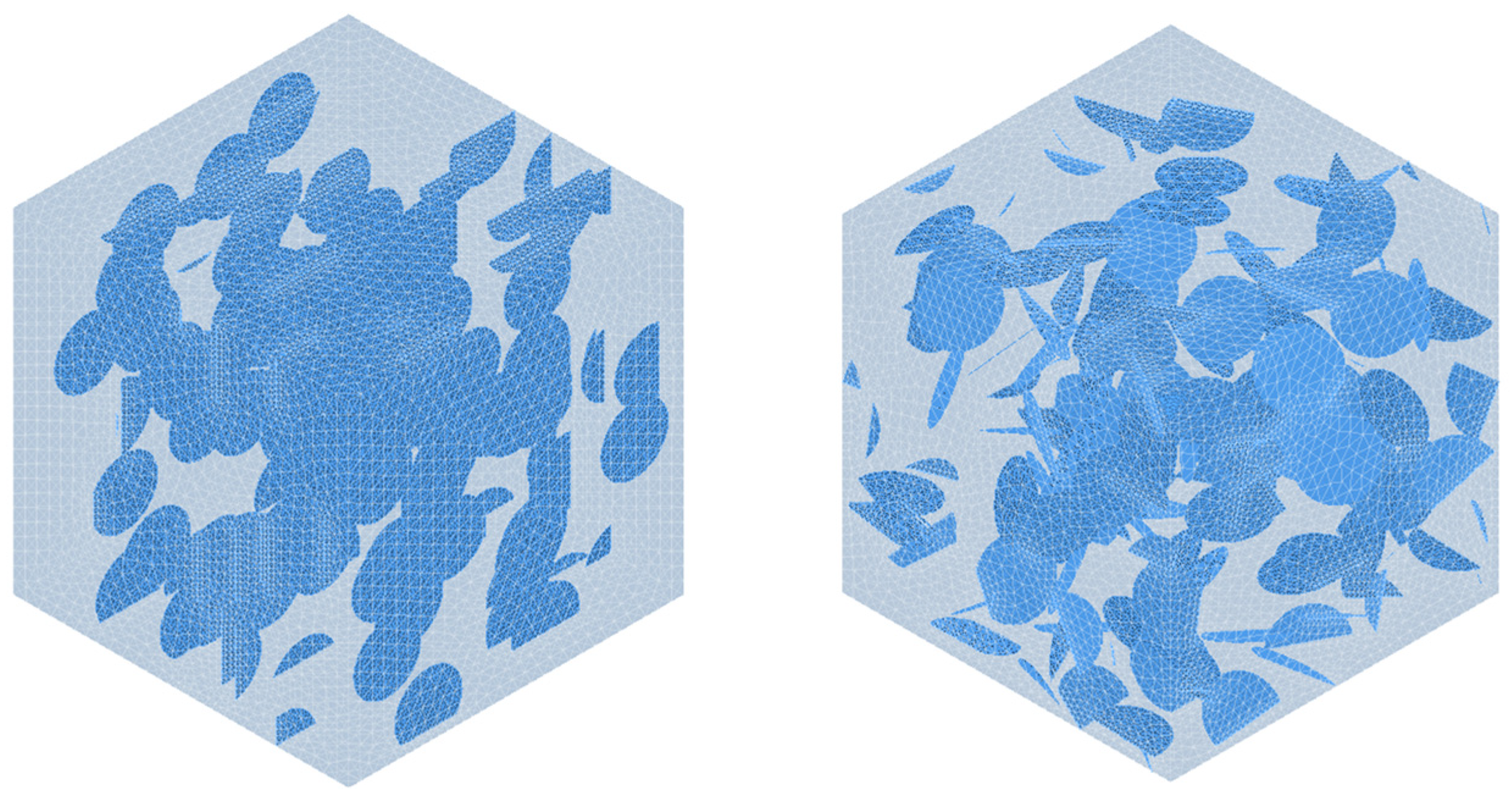
4.1. Three-Dimensional Microstructures and Meshes

The Burgers model is implemented in the Mfront (https://tfel.sourceforge.net/gallery.html (accessed on 2 February 2022)) library, offering several advantages and convenient access for Cast3M users. Mfront is a code generator that enables convenient implementation of behavioural laws, which can be efficiently linked to Cast3M to perform finite element calculations [36]. The parameters of the Burgers model have been calibrated in the previous section. A simple uniaxial creep test with a loading of ${\Sigma }_{11}=1 \mathrm{MPa}$ is performed to verify the perfect agreement between analytical and numerical results for the case where a homogeneous isotropic material is portrayed (Figure 7).

The 3D sample generation procedure is based on a random distribution of inclusions of prescribed shape and size in a box [37,38]. Disc-shaped cracks of zero thickness were introduced as they are suitable for direct comparisons with analytical results [7,39,40]. From this viewpoint, this generation procedure constitutes an improvement with respect to the previous method in which the inclusions are constituted of volume inclusions of non-zero thickness [19]. The geometry of the REV is periodic, which implies that periodic boundary conditions can be applied. The 3D meshes with tetrahedral elements were generated according to the selected periodic geometries using automatic software connected to Salome (https://www.salome-platform.org (accessed on 8 February 2022)) (Figure 8). In this study, we use the MG-CADSurf algorithm since it allows us to generate periodic meshes. A mesh refinement is imposed systematically on the surfaces of the cracks by increasing the density of elements to improve the quality of the simulation results. The technique employed to create the cracks is intended to be used with specific interface elements of zero thickness, i.e., double nodes are created at each point of the crack mesh. Here, as the cracks are void, no interface elements are introduced, allowing us to drastically reduce the calculation time at the REV scale [7,40].

A series of test cases were examined featuring an increasing range of crack density parameters, and comparisons were subsequently conducted with analytical results. Starting with relatively low crack density parameters, the four crack density parameters investigated are 0.05, 0.1, 0.15 and 0.2. A progressively increasing number of cracks has been used in order to keep a constant size of the micro-cracks in the REV. Thus, for the corresponding testing cases, the number of cracks used is 50, 100, 150 and 200, respectively. This is applicable to both isotropic and transversely isotropic cases. In order to achieve a consistent isotropic behaviour of the microstructure, the “Fibonacci sphere” method is used, defining a uniform distribution of points on a sphere [41]. The number of these points is equivalent to the number of cracks considered, and the uniformly distributed points on the sphere serve to define the crack orientations in the microstructure (Figure 9). The placement of the cracks, however, remains completely random in all considered cases.

Sufficient numbers of micro-cracks must be included in the solid matrix to ensure a good representativeness, which is why a comprehensive study must be carried out prior to calculations to minimize errors attributable to the REV generation.

The analysis of Figure 10 demonstrates that the microstructures generated are fairly representative, and with minimized deviations, based on the calculation of the effective Young’s modulus as a function of time, whereas the number of cracks involved is varied from 100 to 200 cracks, while the crack density parameter is constant at 0.2. An exponential evolution of the time steps was considered, using 100 time steps in total, ensuring a high concentration of time steps at the early stages of the calculation where there is the greatest variation in the material’s behaviour. The loading applied is a stress of $\sigma =1 \mathrm{MPa}$ with $\mathit{\Sigma }=\sigma {\mathit{e}}_{\mathbf{1}}\otimes {\mathit{e}}_{\mathbf{1}}$, constant with time. Simulations last around 2 h on average in these cases. The number of elements in the meshes in each case majorly affects the simulation time. A mesh convergence study must be carried out to ensure that a sufficient number of mesh elements are used to guarantee optimized results with minimized deviations. In this case, convergence is achieved with a relatively low error of no more than 1% in cases where the number of tetrahedral mesh elements averages 1.5 million. This is shown by calculating the homogenized Young and shear modulus considering microstructures with an increasing number of elements. Consequently, increasing the number of elements beyond this level has no significant effect on the investigated mechanical properties. The calculations are illustrated for the last time step of 100 days (

Table 2. Mesh convergence study considering an isotropic behaviour: computation of the homogenized Young’s modulus and shear modulus. The relative error with respect to the last column is given in parentheses.

	Mesh 1	Mesh 2	Mesh 3	Mesh 4
Number of mesh elements	0.614 M	1.115 M	1.602 M	2.55 M
$E^{hom} \left(\mathrm{GPa}\right)$	2.9877 (2.45%)	2.8543 (1.78%)	2.8941 (0.41%)	$2.9063$
${\mu }^{hom} \left(\mathrm{GPa}\right)$	1.2299 (4.39%)	1.2066 (2.41%)	1.1578 (1.71%)	$1.1781$

and

Table 3. Mesh convergence study considering a transversely isotropic behaviour: computation of the effective out-of-plane Young’s modulus $E_1^{hom}$ and shear modulus ${\mu }_{12}^{hom}$. The relative error with respect to the reference case (last column) is calculated.

	Mesh 1	Mesh 2	Mesh 3	Mesh 4
Number of mesh elements	0.675 M	0.919 M	1.88 M	2.88 M
$E_1^{hom} \left(\mathrm{GPa}\right)$	1.3627 (6.71%)	1.4053 (3.79%)	1.4493 (0.78%)	$1.4607$
${\mu }_{12}^{hom} \left(\mathrm{GPa}\right)$	0.8918 (2.27%)	0.9054 (0.77%)	0.9089 (0.38%)	$0.9125$

), with periodic boundary conditions and the material subjected to a constant stress of $\sigma =1 \mathrm{MPa}$. Two simulations are required to calculate the effective properties: one with $\mathit{\Sigma }=\sigma {\mathit{e}}_{\mathbf{1}}\otimes {\mathit{e}}_{\mathbf{1}}$ for the calculation of the homogenized Young’s modulus, and the second one with $\mathit{\Sigma }=\sigma ({\mathit{e}}_{\mathbf{1}}\otimes {\mathit{e}}_{\mathbf{2}}+{\mathit{e}}_{\mathbf{2}}\otimes {\mathit{e}}_{\mathbf{1}})$ to determine the homogenized shear modulus. For all subsequent simulations, a mesh size of around 1.5 million elements was used. It is important to note that the number of elements is strongly related to the number of cracks, and technically to the crack density, given that the mesh refinement is imposed to accurately describe the cracks.

The specific nature of imposed boundary conditions can also influence the numerical results, and in this case, three boundary conditions were tested: uniform displacement boundary conditions (KUBCs), uniform stress boundary conditions (SUBCs) and finally periodic boundary conditions (PBCs). Modules are calculated by applying a constant load of stress equal to 1 MPa, and the full load is applied from the very first time step. As expected, the calculation results reported in Figure 11 show that the most rigid response is obtained when imposing uniform displacement boundary conditions, while the softest response is obtained when imposing homogeneous stress boundary conditions. Considering that periodic boundary conditions yield an intermediate response both when testing the isotropic and transversely isotropic material, one assumes that they provide the most accurate results, and they will be used as a reference for comparison with analytical results.

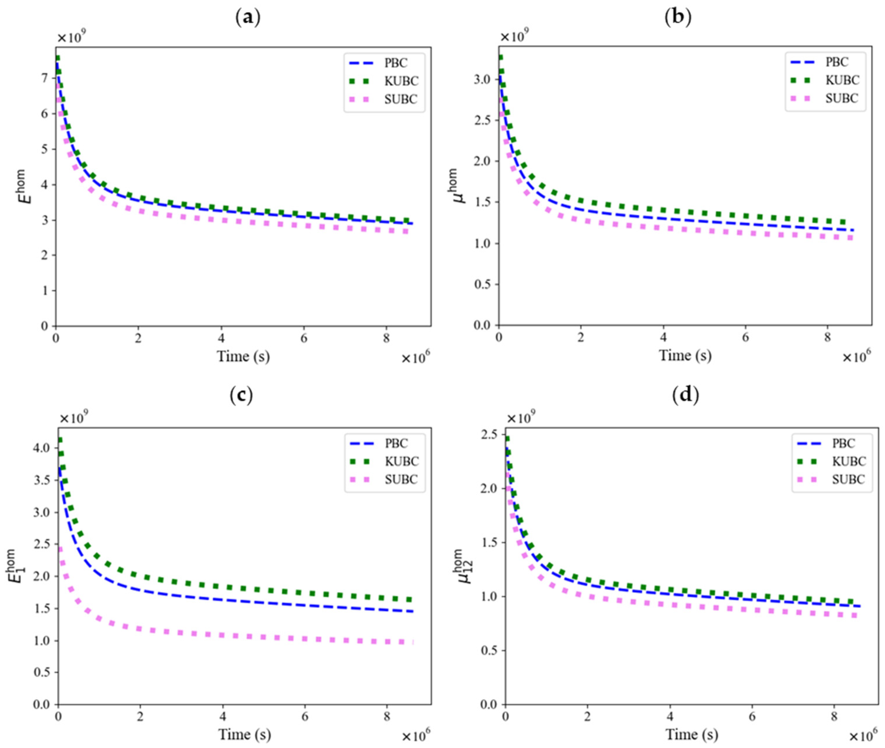
4.2. Transversely Isotropic Case Results

Starting with the transversely isotropic medium and applying periodic stress boundary conditions, a uniaxial creep test is carried out under constant normal stress ${\Sigma }_{11}=1 \mathrm{MPa}$. The time step intervals are identical to the ones defined in Section 4.1. At $\mathrm{t}=0$, the initial conditions correspond to the REV assumed at rest and without any loading. At $\mathrm{t}=0+$, the full loading is applied. Again, the size of REV meshes is around 1.5 million elements, consistent with the mesh convergence study presented in Section 4.1. Comparisons are subsequently conducted between numerical and analytical methods through the calculation of homogenized moduli and the determination of the normal strain as a function of time. In the present case, the moduli affected by cracking are Young’s modulus $E_{11}$ and shear modulus ${\mu }_{12}={\mu }_{13}$, considering the case of parallel cracks where the Ox axis is the direction perpendicular to the corresponding fracture plane in a Cartesian reference coordinate system. The normal strain is calculated as a function of time for the considered crack density parameter (Figure 12). The effective moduli are determined from two separate simulations: the first involving an axial loading at constant stress ${\Sigma }_{11}=1 \mathrm{MPa}$ to calculate the effective Young’s modulus, and the second requiring a deviatoric loading at ${\Sigma }_{12}=1 \mathrm{MPa}$ to assess the effective shear modulus (Figure 12). The analytical approach, however, involves calculating the inverse of the Laplace transform, and thus returning to temporal space. The inverse of the Laplace–Carson transform can be derived directly from the simplified expressions outlined in the previous sections, since it follows a classical form of the Laplace transform, which can be analytically computed. The analytical results are deduced from the equations presented in Section 3.2. For the transverse isotropic case, homogenized moduli are calculated using Walpole’s basis (Equations (13) and (14)), which is subsequently used to determine the Young’s modulus and the homogenized shear modulus.

Initial results show that for the relatively low crack density parameter equal to 0.05, whereby the material still retains a large proportion of its mechanical strength, the numerical and analytical approaches produce very similar results for this case (Figure 12). However, upon investigating the cases with a greater crack density parameter, the numerical results gradually start to deviate from the analytical estimations for the transverse isotropic case, as shown in Figure 13, which depicts the evolution of the creep strain as a function of time for crack density parameters of 0.1, 0.15 and 0.2.

In the final case, where the crack density parameter is equal to 0.2, it becomes clear that the numerical results are no longer comparable with the analytical ones (Figure 13c). In this situation, a different and more appropriate analytical technique is required since the previously described analytical method is only suitable for low crack density parameters. In this regard, previous studies have demonstrated that, in the case of parallel cracks within a linear elastic framework, the differential scheme gives very good results when compared to numerical calculations using the finite element method [35]. This aspect will be investigated in a future contribution.

4.3. Isotropic Case Results

We analyse in this section the creep response of the material when the cracks are randomly oriented, assuming periodic stress boundary conditions. Identical simulation conditions in this section are used to determine the properties of an isotropic medium where the only difference relative to the transverse isotropic case presented in Section 4.1 lies in the definition of crack orientations. The first test is based on an REV with a defined crack density parameter of 0.05 (Figure 14), and the numerical results in terms of normal strain and effective moduli evolutions show good agreement with the analytical ones, similarly to the transverse isotropic results. The analytical solution was obtained using the simplified equations for homogenized moduli in Laplace–Carson space (Equations (9) and (10)), enabling direct calculation of the homogenized Young’s modulus and shear modulus in real time space. The normal strain ${\mathsf{\epsilon }}_{nn}$ is calculated as a function of the Young’s modulus $E^{hom}$ and the applied constant stress $\sigma =1 \mathrm{MPa}$ in LC space (Equation (3)).

For the remaining analyses performed with crack density parameters equal to 0.1, 0.15 and 0.2, the results show that there is a better agreement between the analytical results and the numerical ones than for the transverse isotropic case (Figure 15). Therefore, it can be concluded that the validity domain of the analytical approach for this particular case of isotropic behaviour is extended to include more significantly damaged cases.

Additional investigations were carried out with crack density parameters of 0.3 and 0.4 (Figure 16) for confirming the conclusion of the previous analysis. As shown in Figure 16, the results were consistently similar, maintaining a relatively good agreement between the analytical and numerical approaches even for higher crack density parameters. Consequently, the validity of the analytical solution can be considered as reasonable up to a crack density parameter reaching 0.3–0.4. This is an important conclusion since the reliable analytical solution can be used with confidence to perform structure simulations, thus benefiting from a significant reduction in computational time. The application of this analytical approach within the framework of investigating the behaviour of damaged claystone can be advantageous for a simplified isotropic representation. As mentioned, this applies primarily to situations where cracks are assumed to have a random orientation in some areas of the damaged zone.

5. Discussion

This research suggests an analysis of micro-cracked viscoelastic materials by comparing a numerical approach based on the finite element method and an analytical simplified approach. This analytical approach consists in approximating the effective moduli of the material in the Laplace–Carson space by Burgers models, thereby providing analytical solutions that can be directly compared with the numerical calculations. One key advantage is that the parameters of these approximated Burgers models can be calculated as a function of the parameters of the linear viscoelastic models defining the behaviour of the sound material and the crack density parameter. This makes the approach adapted for structure simulations as the models can be implemented as a classical behaviour law. The presented results include uniaxial creep tests, involving the calculation of normal strain as well as the evaluation of homogenized moduli affected by the cracking. The analysis for the transverse isotropic medium shows that the analytical approach only seems satisfactory for crack density parameters below around 0.1–0.15. For higher values, the numerical calculations diverge significantly from the analytical results. It is envisaged to investigate the use of more adapted analytical approaches for this case of parallel cracks such as methods deriving from the differential scheme, as it has previously proven to be valid in a linear elastic context [35].

In the case of an isotropic crack distribution, the analytical results were consistently closer to the numerical ones, including in the case of a crack density parameter up to 0.4. In that case, although the material is considered severely damaged, the analytical calculations were still in line with the numerical results, proving the validity of this method in the specific case of randomly oriented cracks in an isotropic medium.

Numerical approaches can be used to increase the crack density parameter to values greater than 1, which opens up possibilities for investigating phenomena occurring in severely damaged materials. As crack density increases, interactions between cracks inevitably intensify, creating microstructures highly dense in fractures. This can lead to the formation of preferential cracking paths, particularly in the case of randomly oriented cracks, generating a percolation phenomenon that is particularly interesting to explore. It would also be pertinent to consider irregular crack shapes to achieve an accurate representation of cracks in reality. Numerical approaches provide a means of studying more complex crack geometries, which can be compared with the conventional example of penny-shaped cracks. Overall, this study highlights the importance of combining analytical and numerical approaches to fully understand the behaviour of cracked materials, taking into account the respective limitations of each method and exploiting the results to obtain a more accurate and representative model.

6. Conclusions

In this study, the combined application of numerical and analytical approaches was explored in order to characterize the behaviour of the cracked viscoelastic COx claystone. This approach features a concrete application for representing the argillite in the context of the Cigéo project devoted to the storage of nuclear waste. Indeed, cracking of the host rock results from the excavation of the tunnels at 500m below ground level. Given the significant creep properties of the claystone, it is essential to account for both cracking and creep of the material. For simplification purposes, a linear viscoelastic behaviour has been adopted, which allows the application of the Laplace–Carson transform. This reduces the problem to a linear elastic behaviour in the Carson space, greatly simplifying the equations to provide straightforward analytical solutions. The Burgers model is selected as the viscoelastic model as it is capable, with a minimum number of parameters, of providing an appropriate representation of the behaviour of the undamaged COx claystone.

In addition, two different cases were investigated, one involving an isotropic distribution of cracks in the solid matrix, resulting in an isotropic behaviour, and the second featuring a parallel distribution of cracks, resulting in a transversely isotropic behaviour of the material. A simplified approach was used to calculate the homogenized moduli, assuming that the macroscopic behaviour of the damaged material conforms to a Burgers model. This approach makes the identification of the model parameters feasible as a function of the parameters of the sound material and the crack density parameter, using simplified analytical expressions. While examining the transversely isotropic case, increasing the crack density parameter induces a progressive divergence in the approaches, and the analytical and numerical solutions are no longer fully comparable for parameters greater than 0.1–0.15. Advanced numerical studies can be pursued by investigating the material’s behaviour at crack densities greater than 0.2. The objective is to represent the behaviour of a severely damaged material, particularly in the context of describing the damaged zone behaviour for applications associated with the Cigéo project. With this background, two different cases of crack orientations are examined, consistent with in situ observations of the damaged zone. The first case involves a parallel crack distribution with a preferential orientation, while the second features randomly oriented cracks in an isotropic matrix.

Ultimately, further testing with an isotropic medium showed that the analytical solution gives fairly good results even for relatively high crack density parameters, as shown when comparing it with the numerical results. Potentially, time-consuming calculations of complex microstructures using the finite element method can be replaced by analytical solutions, as they have been proven to provide very similar results in certain conditions. Furthermore, this approach would provide basic solutions for multi-scale applications, in order to obtain the macroscopic response of a cracked material. Further investigations would involve examining different crack geometries, given that the crack shape can influence the calculations of the effective properties of the material. Alternatively, different analytical approaches can be explored, particularly in the case of aligned cracks exhibiting a transverse isotropic behaviour. This could involve the use of homogenization schemes that could produce results more consistent with the numerical ones. The application of the differential scheme would be relevant, given its proven validity in the case of a transversely isotropic medium in a linear elastic framework [19]. The application of this approach with the differential scheme in a linear viscoelastic context is currently being investigated and will be discussed in a forthcoming contribution.

References

1. Andra Dossier d’options de Sûreté—Partie Exploitation (DOS-EXPL), Technical Report, 2016.
2. De La Vaissière, R.; Armand, G.; Talandier, J. Gas and water flow in an excavation-induced fracture network around an underground drift: A case study for a radioactive waste repository in clay rock. J. Hydrol. 2015, 521, 141–156. [Google Scholar] [CrossRef]
3. Armand, G.; Leveau, F.; Nussbaum, C.; de La Vaissiere, R.; Noiret, A.; Jaeggi, D.; Landrein, P.; Righini, C. Geometry and Properties of the Excavation-Induced Fractures at the Meuse/Haute-Marne URL Drifts. Rock Mech. Rock Eng. 2014, 47, 21–41. [Google Scholar] [CrossRef]
4. Rahal, S.; Sellier, A.; Casaux-Ginestet, G. Poromechanical consolidation and basic creep interactions around tunnel excavation. Int. J. Rock Mech. Min. Sci. 2017, 94, 55–63. [Google Scholar] [CrossRef]
5. Andra Dossier d’options de Sûreté—Partie Après Fermeture (DOS-AF), Technical Report, 2016.
6. Nguyen, S.T.; Dormieux, L.; Pape, Y.L.; Sanahuja, J. A Burger Model for the Effective Behavior of a Microcracked Viscoelastic Solid. Int. J. Damage Mech. 2011, 20, 1116–1129. [Google Scholar] [CrossRef]
7. Bluthé, J.; Bary, B.; Lemarchand, E. Contribution of FE and FFT-based methods to the determination of the effective elastic and conduction properties of composite media with flat inclusions and infinite contrast. Int. J. Solids Struct. 2021, 216, 108–122. [Google Scholar] [CrossRef]
8. Marigo, J.-J.; Maurini, C.; Pham, K. An overview of the modelling of fracture by gradient damage models. Meccanica 2016, 51, 3107–3128. [Google Scholar] [CrossRef]
9. Cao, Y.J.; Shen, W.Q.; Shao, J.F.; Wang, W. A novel FFT-based phase field model for damage and cracking behavior of heterogeneous materials. Int. J. Plast. 2020, 133, 102786. [Google Scholar] [CrossRef]
10. Dormieux, L.; Kondo, D. Stress-based estimates and bounds of effective elastic properties: The case of cracked media with unilateral effects. Comput. Mater. Sci. 2009, 46, 173–179. [Google Scholar] [CrossRef]
11. Tsitova, A.; Bernachy-Barbe, F.; Bary, B.; Hild, F. Experimental and numerical analyses of the interaction of creep with mesoscale damage in cementitious materials. Mech. Mater. 2023, 184, 104715. [Google Scholar] [CrossRef]
12. Mazars, J. A description of micro- and macroscale damage of concrete structures. Eng. Fract. Mech. 1986, 25, 729–737. [Google Scholar] [CrossRef]
13. Dormieux, L.; Kondo, D.; Ulm, F.-J. A micromechanical analysis of damage propagation in fluid-saturated cracked media. C. R. Méc. 2006, 334, 440–446. [Google Scholar] [CrossRef]
14. Castañeda, P.P.; Willis, J.R. The effect of spatial distribution on the effective behavior of composite materials and cracked media. J. Mech. Phys. Solids 1995, 43, 1919–1951. [Google Scholar] [CrossRef]
15. Hershey, A.V. The Elasticity of an Isotropic Aggregate of Anisotropic Cubic Crystals. J. Appl. Mech. 2021, 21, 236–240. [Google Scholar] [CrossRef]
16. Hashin, Z. The differential scheme and its application to cracked materials. J. Mech. Phys. Solids 1988, 36, 719–734. [Google Scholar] [CrossRef]
17. Budiansky, B.; O’connell, R.J. Elastic moduli of a cracked solid. Int. J. Solids Struct. 1976, 12, 81–97. [Google Scholar] [CrossRef]
18. Shao, J.F.; Rudnicki, J.W. A microcrack-based continuous damage model for brittle geomaterials. Mech. Mater. 2000, 32, 607–619. [Google Scholar] [CrossRef]
19. Bluthé, J.; Bary, B.; Lemarchand, E. Closure of parallel cracks: Micromechanical estimates versus finite element computations. Eur. J. Mech. A/Solids 2020, 81, 103952. [Google Scholar] [CrossRef]
20. Ricaud, J.-M.; Masson, R. Effective properties of linear viscoelastic heterogeneous media: Internal variables formulation and extension to ageing behaviours. Int. J. Solids Struct. 2009, 46, 1599–1606. [Google Scholar] [CrossRef]
21. Beurthey, S.; Zaoui, A. Structural morphology and relaxation spectra of viscoelastic heterogeneous materials. Eur. J. Mech. A/Solids 2000, 19, 1–16. [Google Scholar] [CrossRef]
22. Schapery, R. A Simple Collocation Method for Fitting Viscoelastic Models to Experimental Data; Graduate Aeronautical Laboratory, California Institute of Technology: Pasadena, CA, USA, 1962. [Google Scholar]
23. Ferreira, L.P.; Lopes, P.C.F.; Leiderman, R.; Aragão, F.T.S.; Pereira, A.M.B. An image-based numerical homogenization strategy for the characterization of viscoelastic composites. Int. J. Solids Struct. 2023, 267, 112142. [Google Scholar] [CrossRef]
24. Eshelby, J.D. The Determination of the Elastic Field of an Ellipsoidal Inclusion, and Related Problems. Proc. R. Soc. Lond. Ser. A Math. Phys. Sci. 1957, 241, 376–396. [Google Scholar]
25. Dormieux, L.; Kondo, D. Approche micromécanique du couplage perméabilité–endommagement. C. R. Méc. 2004, 332, 135–140. [Google Scholar] [CrossRef]
26. Nguyen, S.T. Propagation de Fissures et Endommagement par Microfissures des Matériaux Viscoélastiques Linéaires non Vieillissants. Ph.D. Thesis, Université Paris-Est, Créteil, France, 2010. Available online: https://pastel.hal.science/tel-00598511 (accessed on 10 May 2022).
27. Cuvilliez, S.; Djouadi, I.; Raude, S.; Fernandes, R. An elastoviscoplastic constitutive model for geomaterials: Application to hydromechanical modelling of claystone response to drift excavation. Comput. Geotech. 2017, 85, 321–340. [Google Scholar] [CrossRef]
28. Mánica, M.; Gens, A.; Vaunat, J.; Ruiz, D.F. A time-dependent anisotropic model for argillaceous rocks. Application to an underground excavation in Callovo-Oxfordian claystone. Comput. Geotech. 2017, 85, 341–350. [Google Scholar] [CrossRef]
29. Zhang, C.; Rothfuchs, T. Experimental study of the hydro-mechanical behaviour of the Callovo-Oxfordian argillite. Appl. Clay Sci. 2004, 26, 325–336. [Google Scholar] [CrossRef]
30. Armand, G.; Conil, N.; Talandier, J.; Seyedi, D.M. Fundamental aspects of the hydromechanical behaviour of Callovo-Oxfordian claystone: From experimental studies to model calibration and validation. Comput. Geotech. 2017, 85, 277–286. [Google Scholar] [CrossRef]
31. Nguyen, S.T. Generalized Kelvin model for micro-cracked viscoelastic materials. Eng. Fract. Mech. 2014, 127, 226–234. [Google Scholar] [CrossRef]
32. Nguyen, S.T.; Vu, M.; Vu, N.; Thi Thu Nga, N.; Gasser, A.; Rekik, A. Generalized Maxwell model for micro-cracked viscoelastic materials. Int. J. Damage Mech. 2015, 26, 697–710. [Google Scholar] [CrossRef]
33. March, N.G.; Gunasegaram, D.R.; Murphy, A.B. Evaluation of computational homogenization methods for the prediction of mechanical properties of additively manufactured metal parts. Addit. Manuf. 2023, 64, 103415. [Google Scholar] [CrossRef]
34. Walpole, L.J. Elastic Behavior of Composite Materials: Theoretical Foundations. In Advances in Applied Mechanics; Yih, C.-S., Ed.; Elsevier: Amsterdam, The Netherlands, 1981; Volume 21, pp. 169–242. [Google Scholar]
35. Bluthe, J. Modélisation Couplée et Simulation Numérique des Phénomènes de Colmatage des Argilites. Ph.D. Thesis, Paris Est, Créteil, France, 2019. Available online: http://www.theses.fr/2019PESC1027 (accessed on 27 November 2021).
36. Helfer, T.; Michel, B.; Proix, J.-M.; Salvo, M.; Sercombe, J.; Casella, M. Introducing the open-source mfront code generator: Application to mechanical behaviours and material knowledge management within the PLEIADES fuel element modelling platform. Comput. Math. Appl. 2015, 70, 994. [Google Scholar] [CrossRef]
37. Bary, B.; Bourcier, C.; Helfer, T. Analytical and 3D numerical analysis of the thermoviscoelastic behavior of concrete-like materials including interfaces. Adv. Eng. Softw. 2017, 112, 16–30. [Google Scholar] [CrossRef]
38. Honório, T.; Bary, B.; Benboudjema, F. Multiscale estimation of ageing viscoelastic properties of cement-based materials: A combined analytical and numerical approach to estimate the behaviour at early age. Cem. Concr. Res. 2016, 85, 137–155. [Google Scholar] [CrossRef]
39. Charpin, L.; Ehrlacher, A. Estimating the poroelastic properties of cracked materials. Acta Mech. 2014, 225, 2501–2519. [Google Scholar] [CrossRef]
40. Vasylevskyi, K.; Drach, B.; Tsukrov, I. On micromechanical modeling of orthotropic solids with parallel cracks. Int. J. Solids Struct. 2018, 144–145, 46–58. [Google Scholar] [CrossRef]
41. Hannay, J.H.; Nye, J.F. Fibonacci numerical integration on a sphere. J. Phys. A Math. Gen. 2004, 37, 11591. [Google Scholar] [CrossRef]
Figure 1. Schematic representation of the Burgers model.
Modelling 05 00033 g001
Figure 2. Identification of the Burgers model parameters based on experimental creep test results.
Modelling 05 00033 g002
Figure 3. Schematic representation of randomly oriented crack distribution in a solid matrix.
Modelling 05 00033 g003
Figure 4. Effective moduli calculation as a function of crack density, considering an isotropic crack distribution in the solid matrix.
Modelling 05 00033 g004
Figure 5. Parallel crack distribution in the solid matrix.
Modelling 05 00033 g005
Figure 6. Determination of the moduli affected by cracking for the transversely isotropic case in the Walpole basis as a function of crack density.
Modelling 05 00033 g006
Figure 7. Cast3M verification of the conformity between the implemented Burgers model and the analytical results, obtained following a creep test using the undisturbed material.
Modelling 05 00033 g007
Figure 8. Microstructure meshes generation in Salome with a crack density equal to 0.1 with 100 cracks distributed in the solid matrix (ratio of crack radius to cube side length is 20 / 200 ), considering a parallel crack distribution (left) and an isotropic crack distribution (right) in the REV.
Modelling 05 00033 g008
Figure 9. Even distribution of points across the sphere in order to define crack orientations in the microstructure and ensure an isotropic behaviour.
Modelling 05 00033 g009
Figure 10. Evaluation of REV representativity by varying the number of cracks distributed in the microstructure while keeping a constant crack density   ϵ = 0.2 . The effective Young’s modulus in the direction normal to the cracking plane for the transverse isotropic case is calculated (left) as well as the effective Young’s modulus for the isotropic case (right), and periodic stress boundary conditions were applied.
Modelling 05 00033 g010
Figure 11. Effects of the applied boundary conditions KUBCs, SUBCs and PBCs on the calculated homogenized Young’s modulus (a) and shear modulus (b) for the isotropic medium, and on the Young’s modulus in the direction normal to the crack (c) and the effective shear modulus (d) for the transverse isotropic case, as a function of time.
Modelling 05 00033 g011
Figure 12. Comparison between numerical and analytical results with ϵ = 0.05 and a number of cracks equal to 50. The strain under constant stress loading is calculated (a) as well as the homogenized moduli affected by the cracking for the transverse isotropic medium (b,c).
Modelling 05 00033 g012
Figure 13. Creep strain calculation featuring numerical–analytical comparisons with an increasing crack density of 0.1 (a), 0.15 (b) and 0.2 (c).
Modelling 05 00033 g013
Figure 14. Comparison between numerical and analytical results with   ϵ = 0.05 . The normal strain under constant stress loading is calculated (a) as well as the effective Young’s modulus (b) and the shear modulus (c) for an isotropically cracked medium.
Modelling 05 00033 g014
Figure 15. Influence of increasing the crack density on the normal strain determined from a creep test with ϵ equal to 0.1 (a), 0.15 (b) and 0.2 (c). Numerical results are then compared to the analytical ones for the tested cases.
Modelling 05 00033 g015
Figure 16. Results of a uniaxial creep test in an isotropic medium considering crack densities of 0.2, 0.3 and 0.4.
Modelling 05 00033 g016