Abstract
Metal creep has been a subject of extensive study for more than 110 years because it affects the useful life of engineering components operating at high temperatures. This is even more true with ever-increasing operating temperatures of propulsion/power-generation systems and the environmental regulations to reduce greenhouse emissions. This review summarizes the recent development in creep modeling with regards to creep strain evolution, creep rate, creep ductility, creep life, and fracture mode, attempting to provide a comprehensive mechanism-based framework to address all the important creep phenomena and the long-standing issue of long-term creep life prediction with microstructural evolution and environmental effects.
1. Introduction
Creep refers to time-dependent deformation under sustained loading, which is an important subject in engineering design for high-temperature applications. The phenomenon was first observed by Andrade (1910) [1,2], more than 110 years ago. To date, it remains to be and becomes even more critical to evaluate high-temperature components, especially those operating in gas turbines, steam turbines, pressure vessels, etc., as they tend to be exposed to higher and higher temperatures to meet the CO2 emission reduction target.
Depending on the application, engineering creep failure criteria could be given as [3]:
- creep strain to a specified level, e.g., 1%.
- creep life for intended hours of service, e.g., 100,000 h.
Type I criteria apply to cases where the change of shape/dimension exceeds the tolerance limit to cause unwanted interference with adjacent components, e.g., elongation of rotating turbine blades rubbing the casing. Type II criteria generally apply to static high-temperature components for which economic safe-operation is of paramount concern. Then, in design data sheets, material creep strength can be defined either as the stress to cause a certain amount of creep strain for a prescribed time, e.g., 100 h, 1000 h, 10,000 h, etc., or as the stress to cause creep rupture for a prescribed life, e.g., 100,000 h, at given temperatures. These data are often obtained through creep coupon testing. Sometimes, creep strength is also defined in terms of the temperature capability for a given performance (time at stress). For example, the creep strength of a new generation single crystal Ni-base superalloy is marked by an increase of 25–30 °C for 1000 h to reach 1% strain at 137 MPa [4].
In addition, modern machinery generally operates under complex loading conditions consisting of both mechanical and thermal load cycles, which would result in creep-fatigue interaction, or thermomechanical fatigue. The description of such complicated problems relies on a thorough understanding of deformation and damage mechanisms in both fatigue and creep. However, due to the limited space, the topic of creep-fatigue interaction will be left out of the scope.
In general, creep design often concerns the following questions:
- What is the creep deformation behavior, i.e., creep strain/rate as a function of time, stress, and temperature, to the point of rupture?
- How does the creep life vary with stress and temperature?
- What are the effects of chemical composition and microstructure (via manufacturing process and heat treatment, etc.) on the material’s creep resistance?
- How does the material microstructure change during long-time service at high temperatures and, if changed, what is its effect on the material’s creep performance?
- Does the operating environment have an effect on the material’s creep performance?
Numerous studies have been dedicated to addressing the above questions in the past, but mostly on one or two aspects in each case study (article). Some fundamentals of creep have been covered in a recent book [5], yet unresolved issues still need further discussion. This article summarizes the observed creep phenomena and reviews the state-of-the-art in creep modeling. Particularly, emphasis is given to the mechanism-based modeling approach describing the observed phenomena of creep deformation, fracture mode, and life with constitutive equations derived from the underlying mechanisms for complex engineering alloys over a wide range of stress and temperature conditions. This way, it is hoped that design engineers can have a full physical picture of creep in order to achieve optimal design for various industrial applications.
2. Creep Phenomena
In this section, creep phenomena are depicted by empirical equations, similar to when they were first observed. Interpretations of these phenomena will be made using mechanism-based creep models with experimental data discussed in later sections.
2.1. Creep Deformation
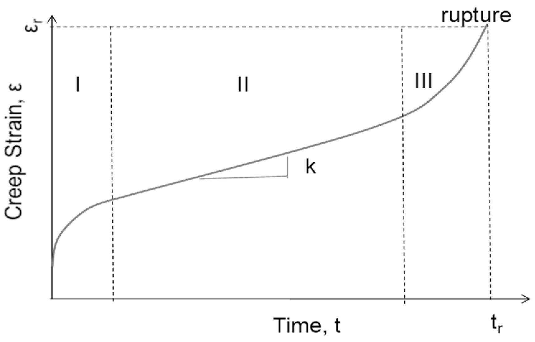
Creep deformation occurs in the homologous temperature range of 0.3–0.9 T/Tm, where T is the application temperature and Tm is the material’s melting temperature in degree Kelvin. It generally proceeds in three stages: (I) primary; (II) secondary, or the steady-state; and (III) tertiary stage, as schematically shown in Figure 1. In the primary stage, creep rate is decelerating; in the secondary stage it exhibits a nearly constant creep rate, which is often known as the minimum creep rate; and in the tertiary stage creep rate is accelerating to the point of rupture at last. Creep deformation can occur under stresses well below the material’s yield strength. Therefore, it is distinguished from rate-independent plasticity, even though both lead to permanent shape change. Basically, all creep phenomena such as creep strain, creep rate, creep life, and creep ductility are attributes of the creep curve (process). Metallurgical examinations using scanning electron microscopy (SEM) and transmission electron microscopy (TEM) on the microstructure and fracture surfaces of crept specimens are often performed to obtain information for understanding the mechanisms of creep deformation and fracture of the materials.
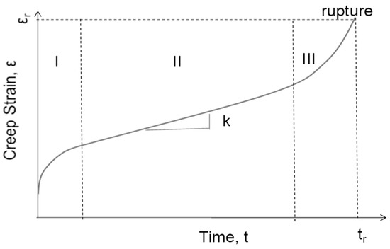
Figure 1.
A schematic creep curve, where tr signifies the time to creep rupture.
Many empirical equations have been proposed to describe creep curves. Norton (1929) and Bailey (1935) proposed a generalized power-law [6,7]:
where t is time, A, n, and m are temperature dependent material constants (in Andrade’s equation, m = 1/3).
Graham–Walles (1955) expanded the Norton–Bailey equation in a series form to describe the three-stage creep deformation (m = 1/3 for the primary stage, m = 1 for the secondary stage, and m > 1 for the tertiary stage) [8].
Evans and Wilshire (1985) proposed a θ-projection method which consists of two exponential terms as [9]
where the θi parameters (i = 1, 2, 3, 4) are polynomial functions of stress (σ) and temperature (T), fitting to the experimental data.
These empirical equations were proposed to depict creep deformation, but bore no meaning on the underlying mechanisms, the rupture (intergranular/transgranular) mode, and time to failure of the creep process, so they are not able to predict creep rupture life unless Type I failure criteria are prescribed.
2.2. Creep Life
Creep rupture life is an important design consideration for high-temperature components such as gas turbine components, pressure vessels, nuclear reactors, etc. Larson and Miller (1952) proposed a data collation method, with the Larson–Miller parameter (LMP) defined as [10]
where CLM is the Larson–Miller constant which often takes a value of ~20 and f(σ) is a function of applied stress.
Using the LMP, the creep strength can be determined from σ-LMP correlation (usually, a polynomial fit). The LMP offers a method to predict creep life assuming that the σ-LMP correlation is a master curve for the material. It implies that short-term data obtained at higher temperatures can be used to predict long-term creep life at lower temperatures, if the LMP of the two conditions is the same. However, due to the scatter in experimental lives, the uniqueness of Equation (3) has never been proven. In addition, the LM method has inherent ambiguities relating to physical mechanisms. Thus, the reliability of the LMP method is still in question. Nevertheless, this method is popularly adopted in creep design, perhaps because of its straightforwardness, as long as enough data are generated to cover the LMP range of application.
Another popular parametric representation of creep strength is the Orr–Sherby–Dorn (OSD) parameter method defined as [11]
where Qc is the activation energy for creep (J·mol−1) and R = 8.314 J·K−1mol−1 is the universal gas constant. POSD is usually a negative number. Similar to the LMP method, the OSD approach also suffers from its empirical nature.
Monkman and Grant (1956) proposed a direct correlation of creep life to the steady-state creep rate, as [12]
where is the minimum creep rate, and
where A0 is a proportional constant, Qc is the activation energy, n is the stress exponent, and σ0 is the normalization stress.
A more sophisticated creep life equation was proposed by Wilshire [13], as
and
where σTS is the material’s tensile strength, k1, k2, u, and v are material constants, and Qc is the activation energy determined from the temperature dependence of έm and/or tr at constant (σ/σTS). Equation (7) describes the creep rupture life, and Equation (8) describes the minimum creep rate. It infers that tr → 0 as σ/σTS → 1, whereas έm → 0 and tr → ∞ when σ/σTS → 0. These equations have been applied to many materials including 9Cr steel [13], 1Cr-1Mo-0.25V steel [14], and Waspaloy [15]. In this method, a linear regression of log (tr·exp(Qc/RT)) vs. log(−log(σ/σTS)) data is employed to obtain the slope u and intercept logk1.
Abdallah et al. performed a critical analysis of the above, and a few more empirical creep lifing equations, on Grade 22 steel creep data from National Institute of Materials Science (NIMS), Japan [16]. They pointed out that in the Wilshire approach, when plotting to obtain k1 and u, multiple linear regimes may exist, which is thought to be due to changes in creep mechanism. To ascertain the stress threshold value of regime-change and determine k1 and u values in different regimes, more creep rupture tests have to be conducted.
For single-mechanism-controlled processes, which occur in a narrow stress range, both LMP/OSD and Wilshire approaches are practically equivalent. But for multi-mechanism creep over a wide range of stress and temperature, the stress-dependence of creep life turns into either a polynomial function (LM) or multi-regime exponential function (Wilshire), which require a lot of creep data to establish the correlation and, therefore, diminish the predictive capability of the model. Most of the time, the above relationships are used to correlate short-term creep test data, and extrapolation of such correlation for long-term creep life prediction is desirable, as a design life of 100,000 h cannot be experimentally-validated before the product is put into the market for commercial competition. The reliability of extrapolation of those short-term empirical relationships is often in question, because many factors, such as microstructural evolution and environment, cannot be fully taken into account in short-term creep tests, which can significantly affect the material’s long-term creep performance. Furthermore, if short-term creep tests are conducted in different mechanism regimes from the long-term service conditions, extrapolations from such tests are not physically warranted. Hence, the prediction of long-term creep properties from short-term experiments is still rated as one of the most important challenges in assessing structural durability, as regarded by the energy sector of the United Kingdom [17]. To fully resolve the issue(s) requires complete understanding of the potential service failure as well as the deformation and failure mechanism(s) in the design creep tests.
2.3. Creep Ductility and Fracture Mode
Creep ductility refers to the strain level at creep rupture, i.e., the last point on the creep curve, as shown in Figure 1. It may also be defined as the cross-sectional area reduction at fracture [18]. To keep in consistency with deformation modeling, the strain definition is used hereafter. One of the notorious effects of creep is to cause an otherwise ductile material to become very “brittle” (with very low ductility) after creep for a period of time under certain stress/temperature conditions. Spindler proposed a creep ductility equation for steels, as [19]
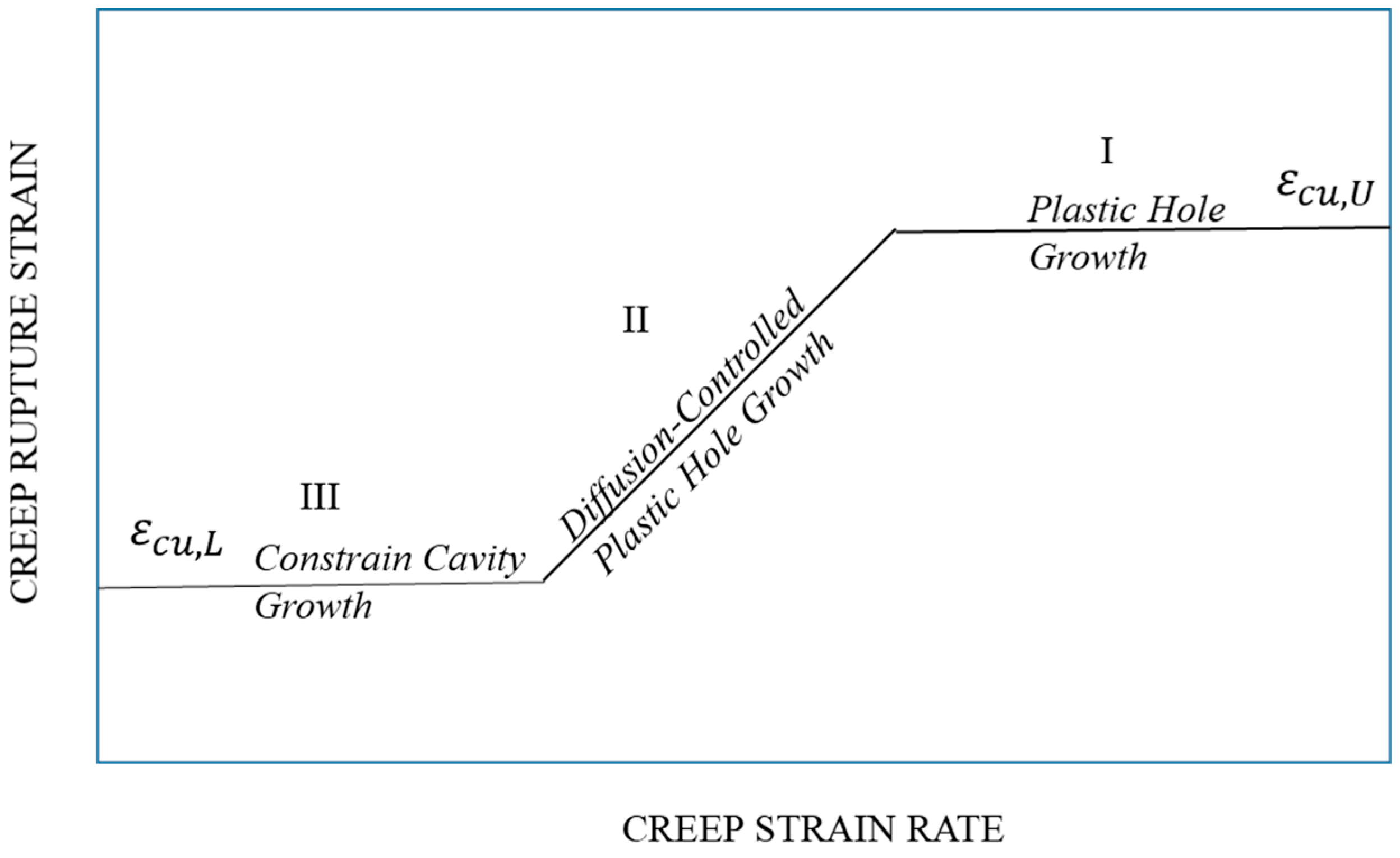
where εcu,L/U are the lower/upper shelf creep rupture strains, C1, n1, and m1 are material constants, Q* is related to diffusion activation energy. Holdsworth used Equation (9) to draw a schematic trending curve [20], as shown in Figure 2, and divided the curve into three regimes: regime I was plastic hole growth leading to ductile dimpled failure; regime II was diffusion-controlled cavity growth and creep ductility decreases with reducing strain rate; whereas in regime III cavity growth was constrained and creep ductility is independent of creep strain rate.
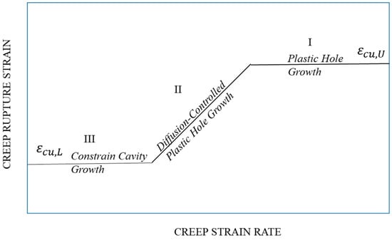
Figure 2.
Variation of creep rupture strain with creep strain rate and damage mechanism in different regimes, redrawn after Holdsworth (2019) [20].
It has been commonly observed that low creep ductility is often associated with intergranular fracture and high creep ductility is associated with transgranular fracture. Equation (9) describes the variation of creep ductility with stress and temperature for steels. All the creep equations in this section were not derived from deformation mechanisms, but rather mathematical correlations of experimental observations, so they are empirical in nature. As one can see, phenomenological equations from Equation (1) to Equation (9) do not relate to each other. If one chose Equations (1) and (2) to depict creep strain, he/she would not know when the life would end. If one chose Equations (3)–(7) to estimate the creep life, he/she would have no idea how creep strain accumulated to the point of fracture. And Equation (9) certainly would not help in understanding the strain accumulation and life. To overcome the conundrum, one ought to resort to understanding the creep deformation and damage mechanisms, and derive physics-based equations to link the above phenomena as discussed below.
3. Creep Mechanisms
Creep deformation mechanisms have been studied extensively using microstructural characterization means, including SEM, TEM, etc. Generally, it has been found that intragranular dislocation movements, such as intragranular dislocation glide (IDG) and intragranular dislocation climb (IDC), diffusion, and grain boundary sliding (GBS), could all operate, leading to time-dependent creep deformation. The dominance of these deformation mechanisms depends on the stress and temperature of application. This is often reflected in the apparent power-law exponent and activation energy.
Based on the thermodynamics and kinetics of slip, an IDG model of exponential stress-dependence was proposed by Kocks, Argon, and Ashby [21]. Mechanism-based models were also developed to show that IDC proceeds by the power-law, as Equation (6), with an exponent of 3 for dilute solution alloys [22,23] and 4.5 for metals with formation of sub-grains [24]. In recent years, dislocation creep models have been further developed based on dislocation density evolution [25] and stacking fault shearing [26]. Creep may also occur as a result of matter flow by either lattice diffusion (Nabarro–Herring creep) or grain boundary diffusion (Coble creep) with a stress exponent of 1 [23]. In addition, GBS may proceed by dislocation glide plus climb along grain boundaries and it is shown to have a stress-exponent of 2 for materials with clean and planar grain boundaries (no grain boundary precipitates) [27]. In complex engineering alloys containing solute atoms and precipitates in the matrix, as well as at grain boundaries interacting with moving dislocations, IDC and GBS tend to have higher stress exponents [28,29,30]. Mechanism models are usually called basic models where creep rate and strain are expressed in terms of mechanisms parameters which are assumptions and theoretically defined. Some “overlapping” exists between the mechanisms. For example, it has been argued that climb-controlled dislocation creep may exhibit a very high stress exponent (~50) in the region, where dislocation glide is commonly believed to dominate (power-law breakdown) [25]. On the other hand, metallurgical evidence of precipitate shearing/cutting do occur, especially in Ni-based superalloys with shearable γ’ precipitates [31]. Generally, the microstructure of a complex engineering alloy is inhomogeneous. While GBS proceeds along grain boundaries, it also causes deformation folds in the neighboring grains at triple junctions, so it appears to be locally constrained. The degree of constraint depends on the intragranular deformation resistance and the formation of wedge cracks at triple junctions. This has been shown by many SEM studies, e.g., [32]. In complex engineering alloys, GBS usually replaces diffusion creep, as linear stress-dependence and grain boundary precipitate denuded zones rarely occur, because grain boundary diffusional migration is inhibited by grain boundary particle-strengthening [33,34]. IDG in complex engineering alloys may also be affected by the presence of strengthening particles through Orowan-looping or precipitate-cutting [35].
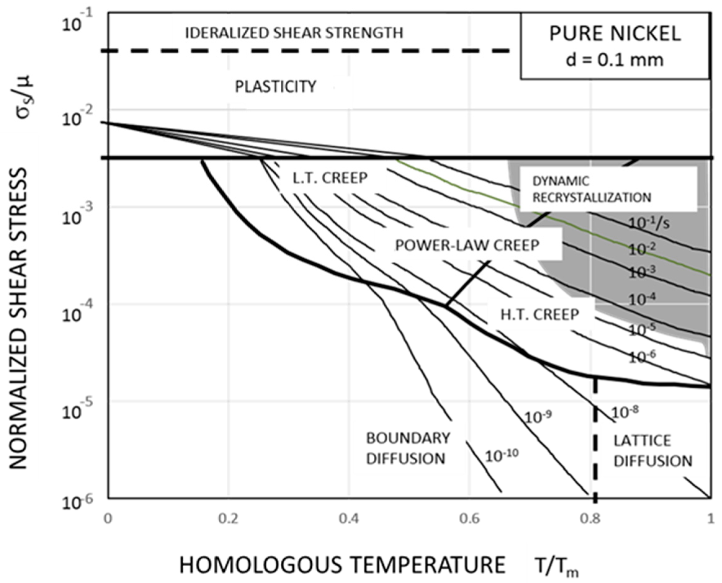
Frost and Ashby (1982) constructed deformation-mechanism maps for many metals [23], which graphically shows the regions of dominance of particular mechanisms in the stress–temperature field with the boundaries being defined by the line of equal contributions from both sides. An example of a deformation mechanism map for pure nickel is shown in Figure 3. Usually, IDC (power-law) creep is dominant in the high-temperature intermediate-stress region. As the stress increases, the exponential stress-dependence of creep rate is manifested, which is called power-law breakdown, meaning that deformation enters into the IDG region. Full discussions of deformation mechanism maps can be referred to Frost and Ashby (1982) for pure metals [21] and Wu (2019) for some engineering alloys [5].
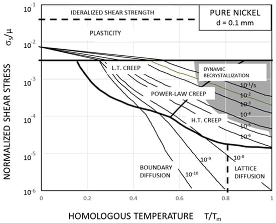
Figure 3.
Deformation-mechanism map for pure nickel, after Frost and Ashby (1982) [23].
It has long been noticed that metals with good tensile ductility could fail with a relatively low elongation after creep for a prolonged period in the homologous temperature range of 0.3 to 0.9 [36]. The reduction in creep ductility is thought to be caused by several grain boundary weakening mechanisms: (1) cavity nucleation and growth by vacancy condensation under stress, either by free diffusion of vacancies [37] or constrained diffusion accommodated by power-law creep [38,39]; (2) grain boundary sliding (GBS) leading to cavity growth from ledges, grain boundary precipitates and/or triple junction (wedge) cracks [32,40,41,42]; and (3) cavity nucleation from Zener–Stroh dislocation pileups against high-angle grain boundaries [43,44].
4. Creep Modeling
Since the mid-twentieth century, a tremendous amount of effort has been spent on creep modeling, because of the importance of the problem in engineering design. Usually, empirical relations were developed first to describe one aspect of creep phenomena. When deviation occurred, as more materials were being examined, either the existing model was amended or new empirical models were proposed to describe the “new” creep data. This is how the Section 2 equations were developed, and they are only a small fraction of what have been proposed in the literature. In the end, one has to manage a set of unrelated empirical relations with many empirical parameters. This requires a significant effort of testing and analysis for a complex engineering alloy.
The basic mechanism models in Section 3 do appear to offer direct calculations of the creep behaviors, as long as the values of mechanism parameters involved are known. The dislocation creep mechanism includes parameters such as dislocation mobility, shear modulus, yield strength, initial dislocation density, dislocation line tension, dynamic recovery constant, work hardening constant etc., in addition to microstructural constants such as the Burgers vector, grain size, or subgrain size. Some of these parameters, such as dislocation mobility, stacking fault mobility, and dynamic recovery, are functions of stress and temperature (the Arrhenius type), and they are not readily available from independent physical testing and measurements to allow predictions to be made without conducting creep tests. The Nabarro–Herring creep equation and Coble creep equation usually predict creep rates in order of the magnitude difference from the observed rates [25]. The dislocation-density-based creep model was applied at stresses above the yield strength for Cu [25], which is not the case in the present study. The basic mechanism models do not specify their operating ranges. Usually, a plethora of mechanisms operate in complex engineering alloys under a given stress/temperature condition, and one has to identify the regions of dominance for each mechanism by comparing their relative contributions to the observed behavior. It is a great challenge to choose the right basic mechanism model from the beginning for engineering design.
To address the creep design questions in Section 1 and link various creep attributes described in Section 2 consistently through a unified approach, this review resorts to deformation-mechanism-based true-stress model (DMTS) [5], as detailed in the following. The DMTS model simulates creep strain accumulation by IDG, IDC, and GBS under true stress conditions with bi-failure-mode criteria, which insinuate that the material may creep-fail transgranularly by intragranular deformation (IDG + IDC) or intergranularly by GBS, whichever reaches its critical strain level first. Hence, creep curve, ductility, life, and fracture mode are evaluated from the partition of these physical mechanisms. By the kinetics, the dominance of each mechanism manifests naturally at each (primary, secondary, and tertiary) stage of creep before unstable deformation (necking) and fracture occurs. Using the mechanism-based approach, the effects of microstructure and environment can also be identified in association with particular deformation mechanisms. Therefore, mechanism-informed insights can be gained through the DMTS model analysis. The model has been applied to many engineering alloys including Waspaloy [45], Mar-M 509 [46], modified Grade 91 steel [47], G115 [48], SA508Gr3 steel [49], Alloy 800 [50], and Haynes® 282TM [51].
Another line of modeling is through machine learning (ML), e.g., [52,53]. Essentially, ML learns from known phenomena (training data) with identified features and make predictions using artificial neural networks (ANN). The advantage is that it can handle a large number of potentially influential parameters as inputs but the disadvantage is that it requires a large amount of data for training. For example, in the work of [53], a total of 90,000 h of stress rupture tests were used for the training/testing data sets. Apparently, ML requires no understanding of the creep deformation and damage mechanisms to yield the output. It is similar to an extended way of phenomenological modeling. As no new phenomena/mechanisms have yet been revealed from ML simulation of creep, the current review omits this part due to the limited scope.
4.1. Deformation-Mechanism-Based True-Stress Model
In general, IDG/IDC and GBS proceed independently in a deformation process, on a microstructural average scale, leading to the total strain rate given by [5,41,42,43,47]
From the review of Section 3, it is understood that each mechanism may be governed by constitutive equations of different forms, some even microstructure sensitive. For consistency and simplicity in mathematics, each mechanism strain rate is formulated as a power-law [5,41,42,43,47]:
where are the creep rates of GBS, IDG, and IDC, respectively; are the proportional rate constants; are the activation energies; p, n, and m are the stress exponents for the respective mechanism; and M is the dislocation multiplication factor [5,41,42,43,47]. It is noted here that, as the first-layer analysis, Equation (11) represents the mechanism strain rates in reduced forms for the mathematical convenience of evaluating the contributions of IDG, IDC, and GBS to the overall creep behavior. For the second-layer analysis, effects of microstructure such as grain size, precipitate size, and distribution may be evaluated using detailed mechanism equations mentioned in Section 3. The exponential stress-dependence of IDG is also reduced to a power-law. The equivalence of the two can be found within the typical experimental scatter band over a narrow stress range [5]. As each mechanism may become dominant only over a narrow stress range, as in Ashby’s deformation mechanisms maps, it is meaningful to evaluate IDG, IDC, or GBS, operating in complex engineering alloys this way. Another reason for using Equation (11) instead of the exact forms of basic mechanism equations is that engineering creep analysis methods have been well-established via regression analysis over log-log and Arrhenius plots. It must be emphasized that the association of power-law to a particular mechanism is not only based on the value of power-exponent and activation energy, but also TEM/SEM microstructures [5,47,51].
As creep deformation is an incompressible flow, the uniaxial true stress-strain evolves with the creep elongation as
where e is the engineering strain and σa is the initial engineering stress.
Substituting the true stress into Equation (11), the integration leads to [5,45,46,47,51]
where k is the absolute minimum creep rate and M* is the tertiary shape factor, the subscript 0 signifies values at t = 0 and σ = σa (in the subsequent text, σ is used to represent the applied engineering stress for brevity).
The transient creep equation for GBS is given by [30]
where β is the transient shape factor and H is the work hardening coefficient of GBS.
Adding up Equations (13) and (16) results in a creep equation that depicts the entire creep curve (Stages I, II, and III) as [5,45,46,47,51]
with
where ε0 is the initial elastic-plastic strain corresponding to offsetting the experimental compliance and and are the primary creep strain and transient time, respectively. Actually, the primary creep time is measured when the primary strain is attained in 99%, such that = 4.6 [30]. Note that Equation (17) is similar to the θ-projection equation, Equation (2), but each component is physically-defined in terms of relevant deformation mechanisms.
From Equation (17), the instantaneous total creep rate is given by [5,45]
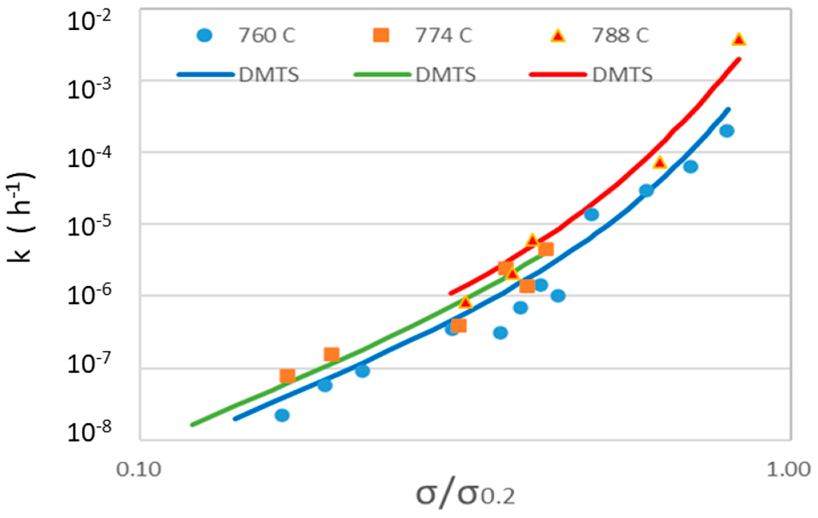
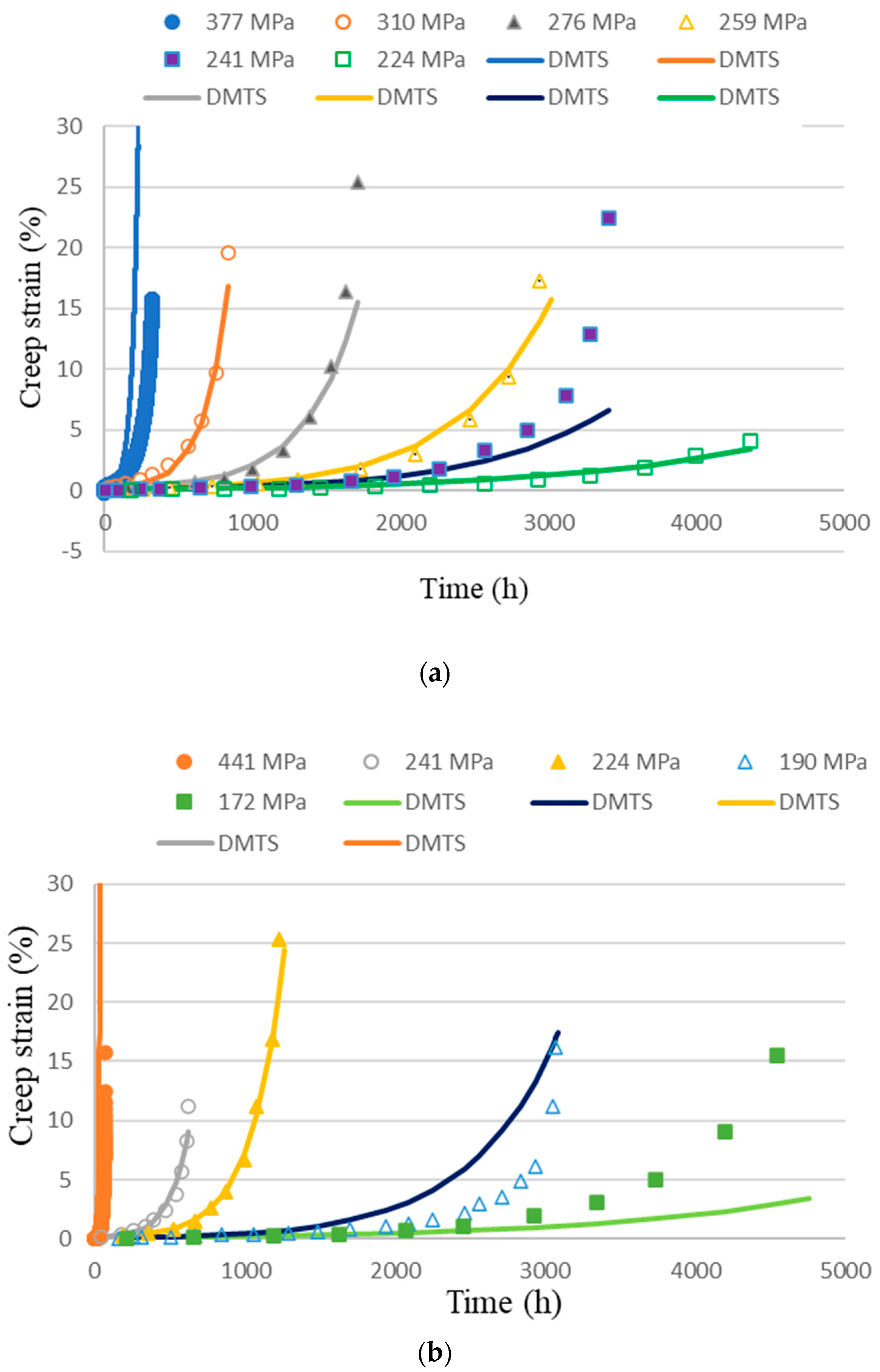
It can be inferred from Equation (19) that the creep rate would first drop from an initial value of k + / to a minimum value, and as the first exponential term diminishes to zero quickly, the creep rate increases exponentially with time when t > . In the tertiary stage, this relationship appears to be log-linear, so that both k and M* can be obtained by linear regression of the tertiary creep data. The absolute minimum creep rate k, which is actually very close to the conventional minimum creep rate, is plotted against σa in a log-log plot, from which the power-law proportional constant and exponent can be obtained for each mechanism. Creep data analysis consists of log-linear /log-log regression and Arrhenius analyses, as detailed in the book [5]. The absolute minimum creep rate vs. normalized stress relationship is shown in Figure 4, and the creep curves predicted by Equation (17) are shown in Figure 5, respectively, in comparison with experimental data for Haynes® 282TM.
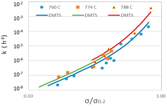
Figure 4.
The absolute minimum creep rate vs. normalized stress of the DMTS model predictions in comparison with experimental data for Haynes® 282TM [51].
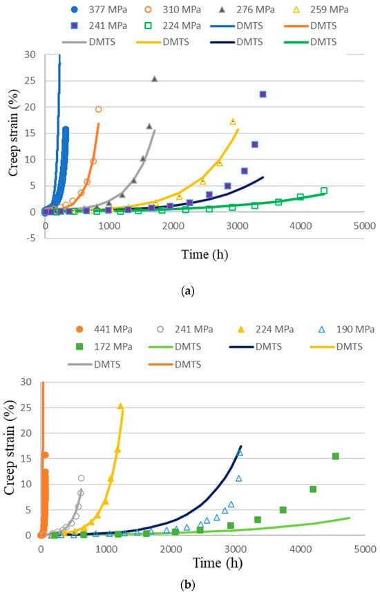
Figure 5.
Predicted creep curves of Haynes® 282TM by the DMTS model in comparison with experimental data at (a) 760 °C and (b) 788 °C [51].
The DMTS model considers the concurrent operation of intragranular deformation (ID = IDG + IDC) and GBS. Naturally, the fracture mode and life will be determined based on which mechanism reaches its ductility limit first. For prediction of long-time creep performance, the initial elastic strain ε0 and the primary strain can be negligible, because tr >> tT, thus, at the time of creep rupture, Equation (17) reduces to [5,51]
where is critical GBS ductility, is critical grain ductility, is failure strain, and is rupture time or creep life. Note that the primary strain arises from grain boundary hardening and it is anelastic in nature and, therefore, not damaging, while represents the ability of grain boundaries to accommodate voids/cracks.
In the case of GBS dominance, intragranular deformation is frozen, i.e., , , and M* = p from Equation (15), then the creep life can be obtained from Equation (17) as [51]
In the case of intragranular deformation dominance, the ID-dominated creep life can be obtained from Equation (17) as [51]
Then, creep rupture occurs whichever of or is reached first, that is, when < , intergranular fracture occurs first, = ; and when ≥ , fracture is caused by exhaustion of intragranular ductility, = . In reality, the fracture may appear to be in a mix-mode, because both ID and GBS occur concurrently, thus the fracture surface may be composed of both grain boundary facets and regions of ductile tearing.
The creep ductility can be calculated by substituting into Equation (17). The variation of creep ductility as a function of stress and temperature is shown in Figure 6 for Haynes® 282TM. Comparing the trend in Figure 2, the GBS ductility (=0.3% for Haynes® 282TM) corresponds to the low-level ductility εcu,L, and the intragranular ductility (=30% for Haynes® 282TM) corresponds to the high-level ductility εcu,U in Figure 2. At high stress, the experimental fracture strain is much higher than the low-level ductility, even though it varies a lot because of the deformation instability under high stresses. The transition between the two levels of creep ductility is a region of mix-mode fracture, with nearly equal partition of IDC and GBS. In Figure 2 the transition is attributed to diffusion-controlled cavity growth. Note that diffusional cavitation has a stress-dependence of power 1 [37], which was not the case for Haynes® 282TM. Fractographic examinations of crept specimens corresponding to the data points in Figure 6 showed that indeed the fracture mode transitioned from intragranular fracture to intergranular fracture as the stress went from high to low [51], which coincided with GBS dominance.
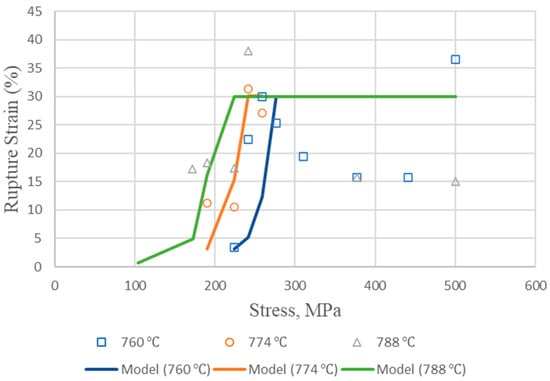
Figure 6.
Comparison between experimental (symbol) and predicted (line) failure strains of Haynes® 282TM at different temperatures [51].
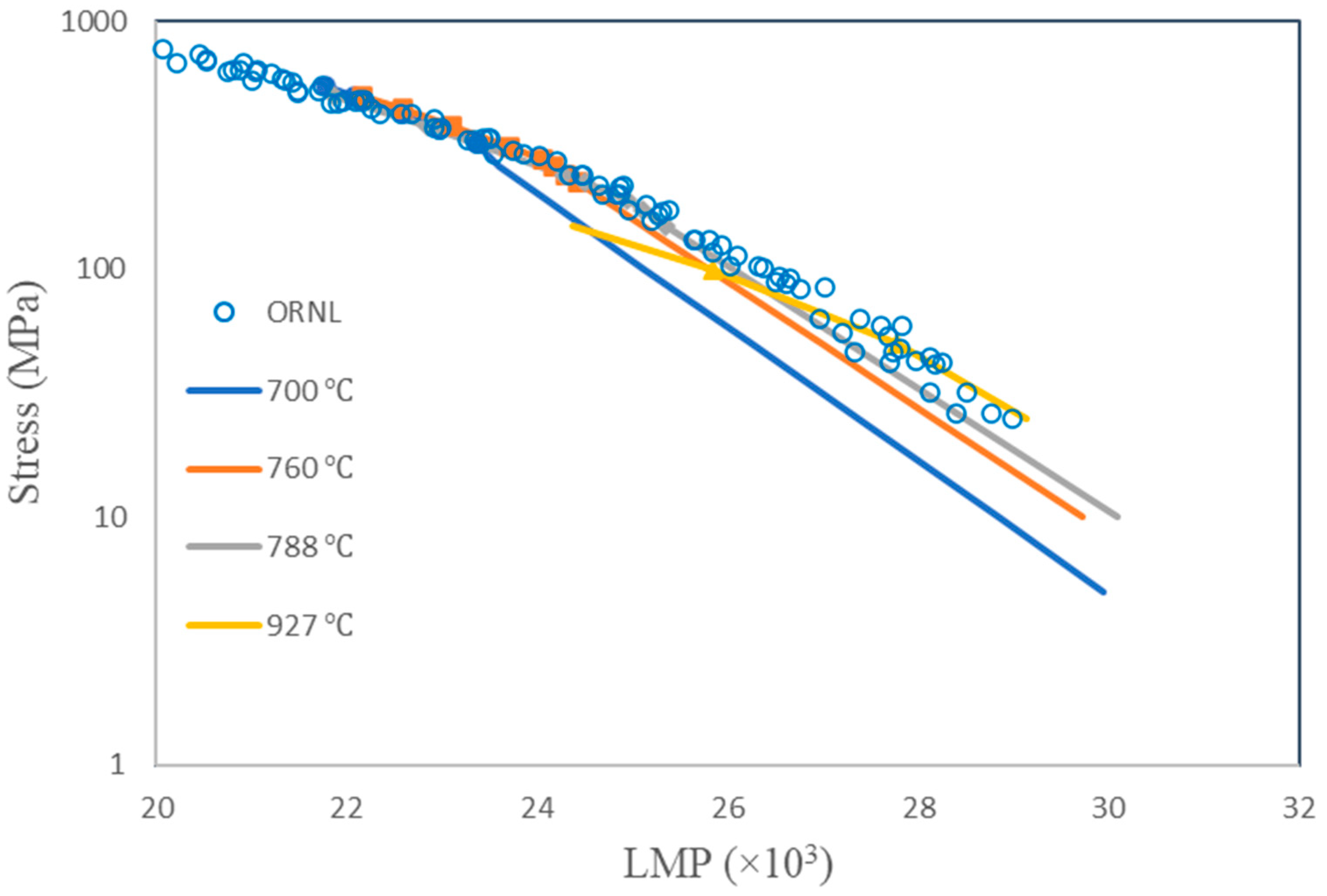
The DMTS model-predicted creep lives of Haynes® 282TM are shown in Figure 7 in comparison with the creep rupture data from Oak Ridge National Laboratory (ORNL) [54] and the National Research Council Canada-Carleton University-Velan collaboration (NRC-CU-Velan) [51]. The DMTS model predictions were made corresponding to each test condition, using the mechanism parameter values given in [51]. First of all, the independent tests proved the observed behavior to be true. Second, the DMTS model predictions agree very well with the experimental data in terms of LMP with CLM = 20. A very high coefficient of determination (R2 = 0.98) is obtained between the DMTS model and the experimental LMP. Unlike the irrelevance of LMP to the underlying mechanisms, the DMTS model carries the mechanism-partitioning information, which is insightful for further discussion.
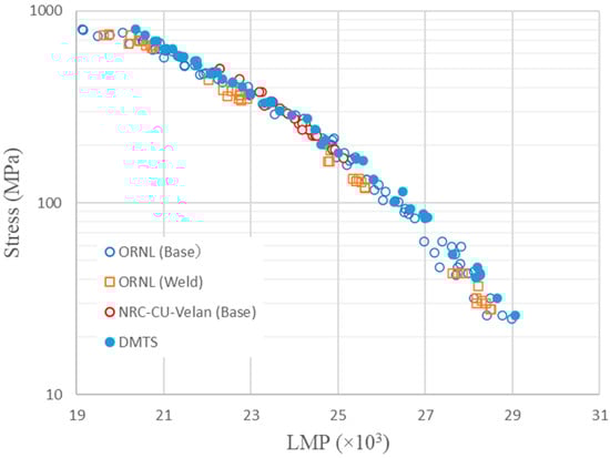
Figure 7.
Larson–Miller plot of the DMTS model predictions for Haynes® 282TM in comparison with the experimental data.
Engineering design by predicting long-term creep life from short-term creep test data using the LMP-σ relation is based on the presumption that this relationship represents a one-to-one correspondence for creep rupture, but it has never been proven by theory and experiments. To investigate this matter, isothermal LMP values at each stress level are computed for different temperatures using the DMTS model, as illustrated in Figure 8. The symbols represent the indicated conditions with a rupture life < 10,000 h, which are typical of short-term tests (ORNL data), assuming that the DMTS model represents the “ideal material” as represented by the set of mechanism parameters, which has no material variability. As one can see, the isothermal short-life LMPs still fall close to the ORNL-data, but the mechanism-based isothermal LMP deviates from the short-term LMP data towards high LMP values, which means that the LMP-σ relation is not a one-to-one correspondence relationship. The deviated lines are governed by GBS. This is the regime where most service conditions fall, but “predictions” are often attempted with short-term creep tests. Short-term tests at higher temperatures tend to generate a larger LMP value at a given stress level, or achieve the target LMP value at higher stresses. For example, the LMP for a service life of 100,000 h at 760 °C is equal to 25.8 × 10³ (with CLM = 20). The same LMP value was produced from the short-term test with a test life of 5058.3 h under 132 MPa at 816 °C (the ORNL test). If the LMP-σ relation were one-to-one, σ = 132 MPa would be taken as the design stress. However, at σ = 132 MPa and T = 1033 K (760 °C), the rupture life of Haynes 282 is 33,144 h, which falls quite short of the target service life of 100,000 h, and hence the design is potentially dangerous. Although the short-term creep tests (<10,000 h) would result in a rather close correlation, caution should be exercised using the empirical short-term LMP method for long-term creep life prediction where GBS plays a dominant role.
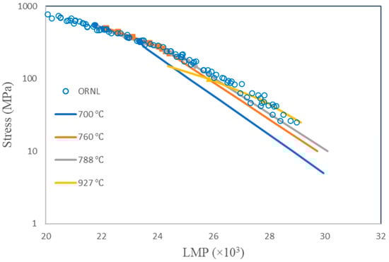
Figure 8.
Comparison of isothermal LMP-σ relations for Haynes® 282 TM.
4.2. Effects of Composition and Microstructure
In general, composition and microstructure have strong effects on material creep performance. Usually, the base metal imparts the basic physical properties, such as elasticity, slip, and diffusion properties, while alloying elements contribute to additional strengthening with solute atoms and precipitates/phase changes. For example, in Ni-base superalloys, this involves γ and γ’ phases and grain boundary M23C6. In heat resistant steels such as modified 9Cr1Mo steels, it involves M23C6 phase, MX phase, and Cu-rich phase. In analytical models, the effect of particle-strengthening is often considered as back-stress through either Orowan-looping or precipitate-cutting mechanisms [28,35]. The effect of grain size, grain boundary precipitates, and grain boundary serrations has also been considered in creep behavior modeling [30,55]. More recent work uses molecular dynamics to simulate dislocation-particle interaction [56,57]. Molecular dynamics simulation of GBS has been performed for pure aluminum without grain boundary precipitates [58]. The dynamic behavior was studied in picoseconds (ps), which is way below the engineering timeframe. As far as of engineering concerns, this article reviews a few examples of how DMTS can be used to delineate microstructure effects.
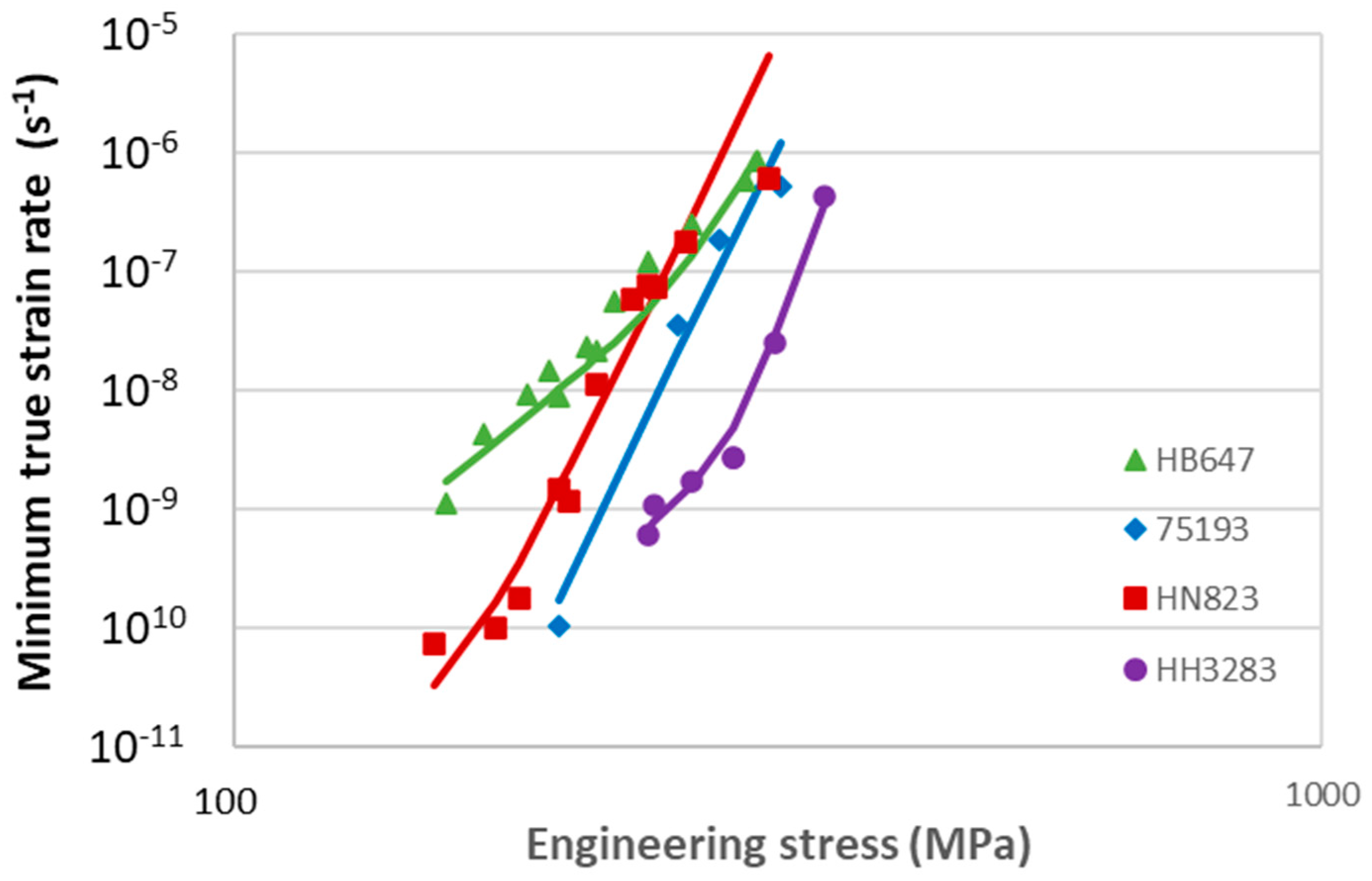
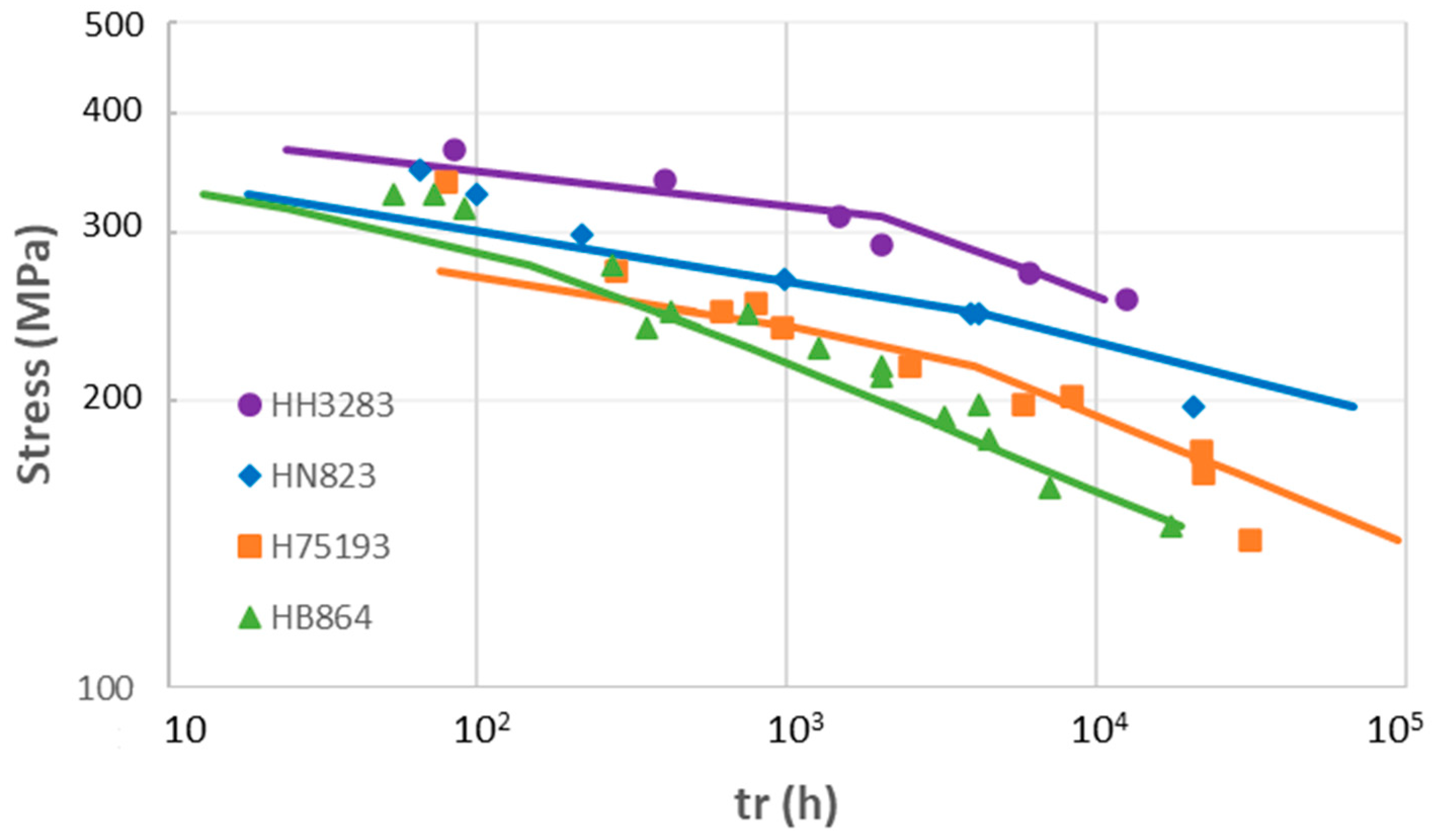
An example of microstructural effect on creep can be found for Alloy 800. A series of Alloy 800 were made with the high/low carbon content and increasing Ti + Al content in ascending order from HB647, 75193, and HN823 to HH3283 [59]. The mechanism parameters for the creep rate in different batches of Alloy 800 at 550 °C are given in Table 1 [50], which are determined to match the minimum creep rate as a function of stress, as shown in Figure 9. The trend of increasing the power-law exponent for the IDG mechanism is consistent with the trend of increasing the Ti + Al content that enables the intragranular γ’ precipitate strengthening mechanism. GBS is assumed to be the same for the high C content alloys, 75193, HN823, and HH3283, with abundant grain boundary Cr23C6 precipitates, while HB647 has a lower resistance to GBS due to its much less C content than the other batches. In these alloys, Ti and Al would have little contribution to GBS, because they do not participate in grain boundary precipitation. The impact of microstructural variation on the rupture life for Alloy 800 is shown in Figure 10. IDG is responsible for intragranular deformation instability (necking) () and GBS causes intergranular fracture ().

Table 1.
Mechanism parameters for different batches of Alloy 800.
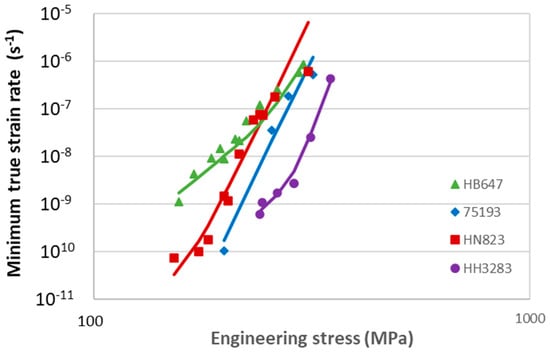
Figure 9.
Creep rates in different batches of Alloy 800 at 550 °C [50].
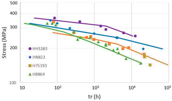
Figure 10.
Creep rupture lives of different batches of Alloy 800 at 550 °C [50].
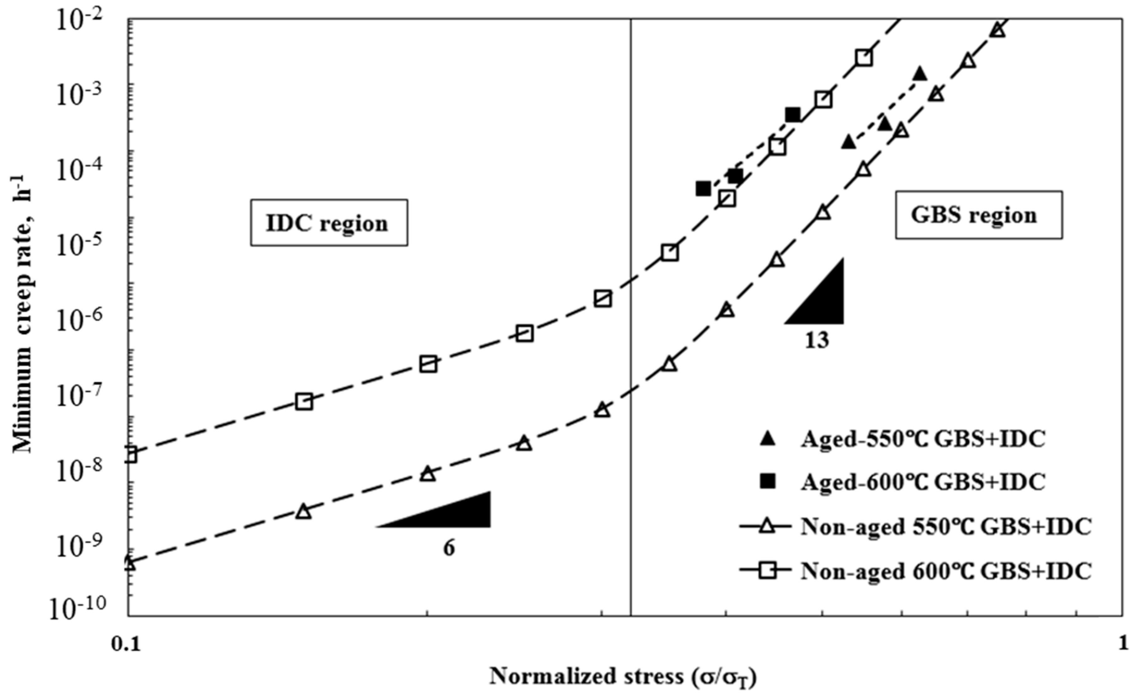
Microstructural evolution in F91 was studied by Zhang et al. through aging heat treatment at 550 °C and 600 °C for up to 5000 h [60]. Notably, a considerable amount of Mo-rich Laves phase formed in F91 during the thermal exposure. The Laves phase Fe2(Mo, W) was found mostly around Cr-rich carbide M23C6, which pinned on the prior-austenite grain boundaries and martensitic lath boundaries, and it coarsened rapidly, leading to premature creep rupture than the unaged F91. By the nature of the Laves phase formation, it would affect GBS much more than IDG. Therefore, assuming that both aged and unaged F91 have the same IDG component unaffected, subtracting the IDG rate from the total creep rate, the GBS+IDC rates are presented in Figure 11. It can be seen that the Laves phase formation proportionally increased GBS, keeping the power-exponent fairly constant because it weakens the pinning effect of M23C6/MX on lath/grain boundaries.
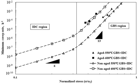
Figure 11.
Comparison of minimum creep rate between aged and unaged F91 coupons without IDG [60].
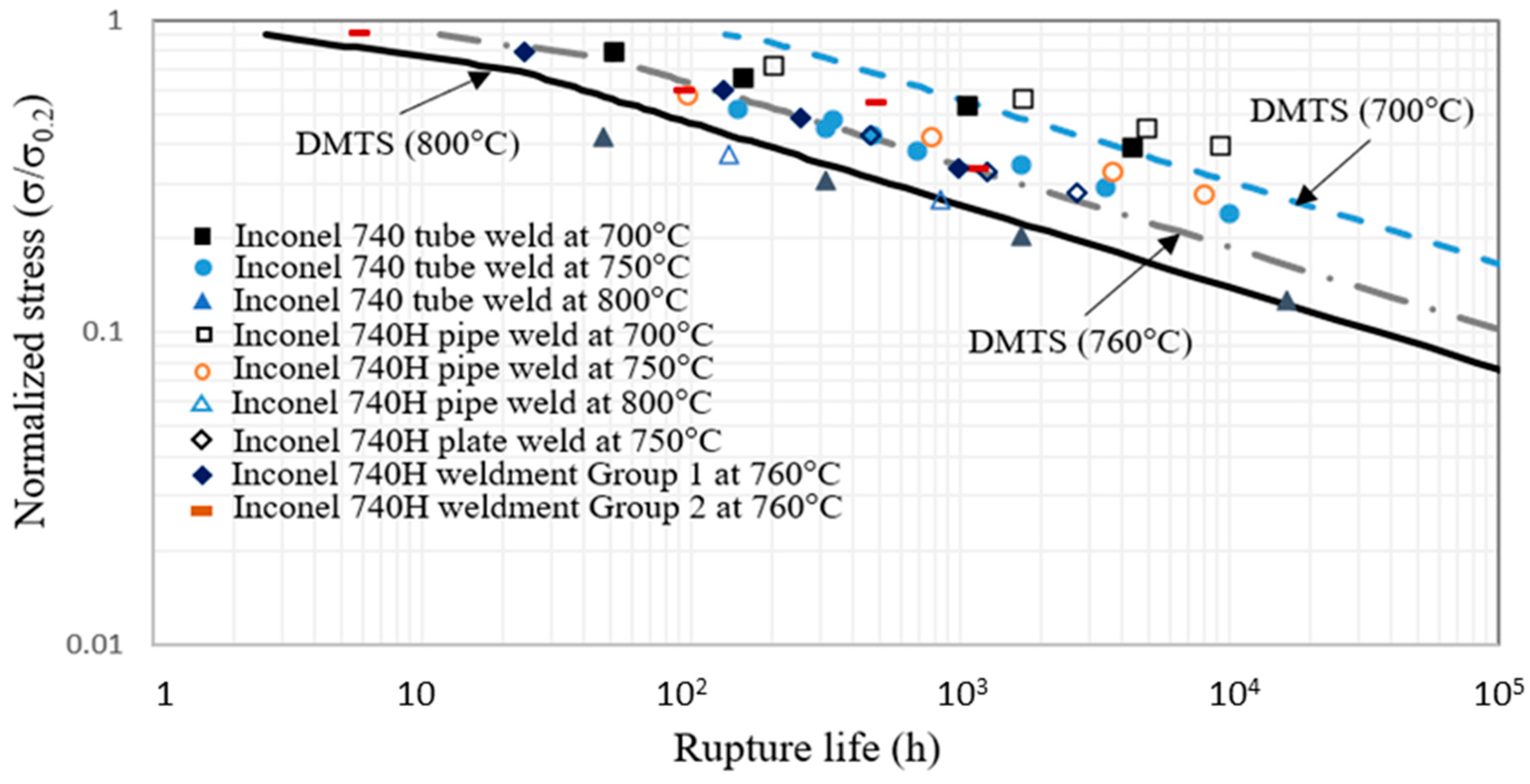
Weldments also represent another form of microstructural change, as compared to the base metal. The creep behavior of Inconel 740H weldment at the temperature of 760 °C was investigated experimentally and analytically using the DMTS model [61]. Inconel 740H is the only material approved by ASME for advanced ultra-supercritical (A-USC) steam turbine applications [62]. Its weldment is as important as the base metal in such applications. The Inconel 740H weldment specimens were prepared with the gas tungsten arc welding (GTAW) technique. In comparison with the base metal, the 740H weld material (after a post weld heat treatment) had apparently wider grain boundaries with coarsened/elongated grain boundary precipitates and γ’ denuded zone. This would potentially weaken the resistance to GBS. The creep data generated on Inconel 740H weldment at 760 °C were analyzed using the DMTS model to delineate intragranular deformation and GBS, and the activation energies for the respective mechanisms were assumed to be the same as Haynes 282, a similar alloy. The DMTS model is used to predict the creep rupture lives within a temperature range of 700–800 °C, as shown in Figure 12. The creep life predictions of the DMTS model for Inconel 740H weldment agree very well with creep rupture test data from both the literature [63] and the NRC-CU-Velan in-house investigation [61]. Although only a few short-term creep data at 760 °C are used to calibrate the mechanism parameters of the DMTS model, the agreement between the DMTS model and test data is remarkably good. The turning points on the DMTS model curves correspond to the transition from intragranular fracture to intergranular fracture, as the stress goes from high to low. The fractured surfaces and longitudinal sections of creep-tested Inconel 740H weldment specimens were examined using SEM, which corroborated the DMTS model inference that the creep failure of Inconel 740H weldment was dominated by GBS with an intergranular fracture mode [61].
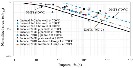
Figure 12.
Creep life predictions of the DMTS model for Inconel 740H weldment at different temperatures in comparison with experimental data and the creep lives of similar materials [61].
The above examples demonstrate that by using the mechanisms-delineation approach, such as the DMTS approach, the effects of composition and microstructure of the materials can be reconciled with the physical deformation mechanisms over a wide range of stress and homologous temperature. This approach removes the ambiguities associated with empirical equations and links the material behavior closely to the physical metallurgy of materials, which should be the focus of future creep studies.
4.3. Environmental Effects
Most high-temperature components operate in open air, which would inevitably suffer from oxidization. The question is, to what extent oxidation may affect the material’s long-term creep performance? Bueno conducted short-term creep tests on 2¼Cr-1Mo steel in vacuum and air, which showed that oxidation had an effect of increasing the creep rate in air as compared to that in a vacuum [64]. Such oxidation-free creep data are rarely available for existing materials, because long-term vacuum creep tests are cost-prohibitive. In conventional creep tests, creep data are obtained with coupon-borne influence of oxidation, but oxidation is a time-dependent process, therefore, empirical extrapolation of short-term creep data for long-term creep life prediction without considering oxidation is questionable. Dyson and Osgerby (1995) considered creep-environment interaction using the continuum damage-mechanics (CDM) approach [65]. However, CDM does not attribute the effect of oxidation to specific deformation mechanisms, that is, CDM does not distinguish intragranular deformation or GBS, so the treatment is still ambiguous.
Oxidation damage can be assessed through post-mortem examination of creep-fracture coupons. In general, the growth of oxide scale, δ, follows the parabolic law as expressed by [66]
where kox is the oxidation coefficient.
When an oxide scale forms, if it is intact, the stress in the oxide scale is given by the composite rule as [5]
where αox and αs are the coefficients of thermal expansion (CTE); Eox and Es are the elastic moduli of the oxide and substrate, respectively; and f is the volume fraction of the oxide scale. For a round bar coupon, f = 2δ/πr, r is the cross-sectional radius. It is noticed that, even when a very thin film forms with f ≈ 0, the stress in the oxide film is magnified by Eox/Es, while the stress in the substrate remains nearly the same. Thus, the oxide scale tends to break first.
If the oxide scale breaks, the load bearing area of the coupon (component) is effectively reduced, and the true stress becomes [66]
Then, following the same derivation procedure of the DMTS model, the same creep strain equation, Equations (14) and (15) can be obtained but with oxidation-modified parameters [66]
The above equations reduce to the basic DMTS model when oxidation is absent and, hence, is called the oxidation-modified DMTS (O-DMTS) model. Equation (26) is shown to predict the creep rate increasing with formation and breaking of oxide scale, which agrees with the experimental observation for F91 [66].
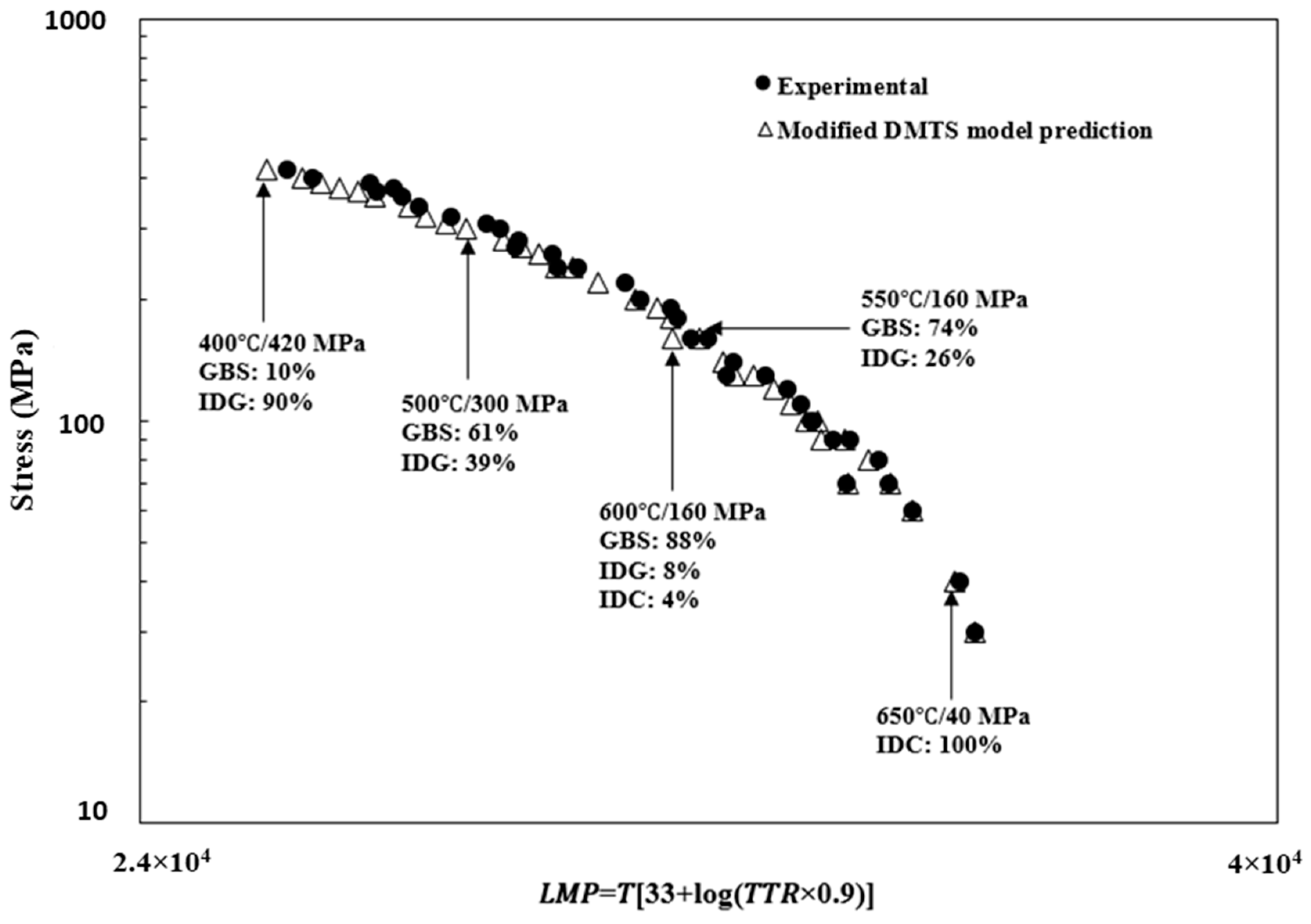
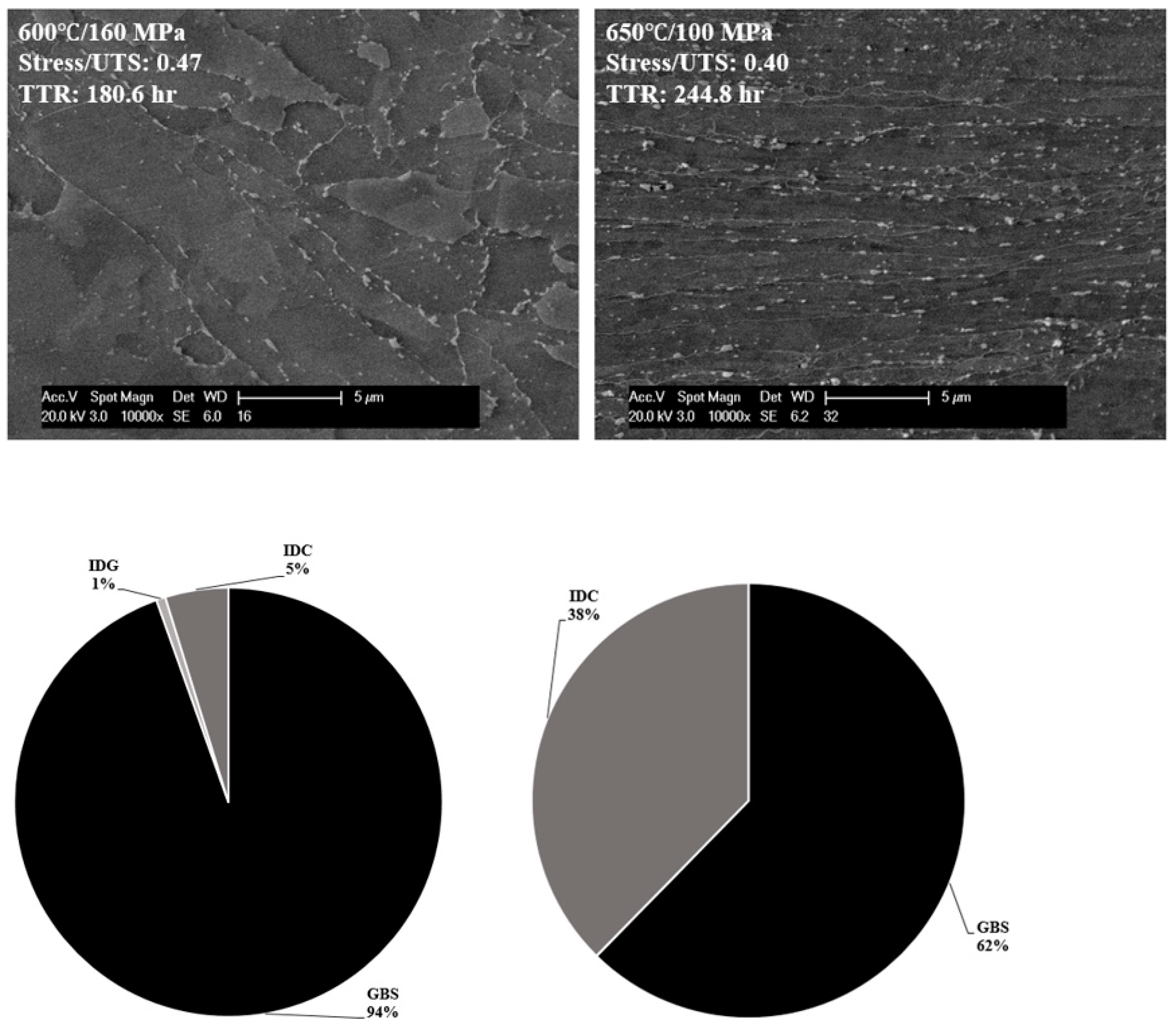
For the purpose of comparison, the predicted creep lives of NIMS Plate MgB by the O-DMTS model are plotted in the LMP diagram in comparison with the experimental data (the rupture lives are taken to be 90% time to rupture (TTR)), because necking occurred at last before rupture. The Larson–Miller constant, CLM, is 33 [67]. Figure 13 shows that the predicted lives agree very well with the experimental data from the NIMS database which contains creep rupture life data up to 105 h. While the LMP method collapse the creep rupture data, the relationship between LMP and stress is not as simple as discussed in Section 2.2; one would have to use polynomials to draw a line (σ vs. LMP relationship) between the data. The problem with polynomial fitting is that it cannot be established without a large amount of data, and extrapolation of polynomials is usually invalid beyond the fitted range. Therefore, long-term creep test data are still needed, when using the LMP method. Interestingly, the oxidation-modified DMTS (O-DMTS) creep model predicted that lives also fall well with LMP, but it is drawn from fundamental deformation mechanisms. Furthermore, the O-DMTS model provides a quantitative partition of GBS/IDG/IDC mechanisms, and it also predicts the rupture mode. Figure 14 shows two microstructures at creep rupture under 600 °C/160 MPa and 650 °C/100 MPa, along with the mechanism pie-chart made up by the contributions from the three mechanisms to the total strain rate. In the 600 °C/160 MPa case, GBS was predominant (~94%) and the microstructure retained its original lath structure, whereas in the 650 °C/100 MPa case, as the model predicted that a significant portion (~38%) of creep deformation would occur by IDC, the lath structure indeed became more elongated (note that the O-DMTS prediction of mechanism partitioning ratio was for the initial condition, and IDC would take more dominance as creep proceeded to the last point of fracture as the true stress increases with elongation). The model predication was thus supported by the metallurgical evidence. Using the O-DMTS model, such pie-charts can be drawn for every creep condition. In this way, engineers are able to understand the physics of failure and identify the failure mode in quantitative detail, whereas the LMP plot does not provide mechanism information, from a life prediction point of view.

Figure 13.
The modified DMTS model prediction of NIMS Plate MgB in LMP plot with experimental data [66].
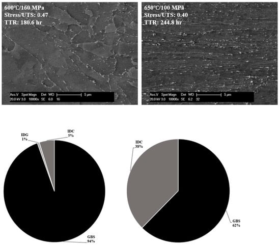
Figure 14.
Microstructure analyses with pie-charts to indicate participating mechanisms [66].
5. Concluding Remarks
This review summarizes creep phenomena including creep strain, creep rate, creep ductility, creep life, and fracture mode, and uses a mechanism-delineation approach via the deformation-mechanism-based true-stress (DMTS) creep model and the oxidation modified DMTS (O-DMTS) creep model to describe/interpret the experimental observations. Over the past 110 years, these phenomena were treated with various empirical equations, but those equations do not connect to each other so they do not provide a complete picture of creep. Especially, the empirical long-term creep life prediction was not warranted for the conditions where the mechanism(s) deviate from the tests from which the data for extrapolation were generated. The main points drawn from this review are summarized below.
As a general creep model for metallic materials, the DMTS model takes the contributions of dislocation mechanisms, such as GBS, IDC, and IDG, into consideration, which enables the description of all salient creep phenomena including creep strain, creep rate, creep ductility, creep life, and fracture mode all together, as demonstrated for complex engineering alloys investigated in this paper and in the references. By the general validity of the physical mechanisms involved, the DMTS model is applicable to all metallic materials.
The DMTS model interprets the microstructural effect with respect to the mechanism contribution that may be affected by the change in microstructure (grain size, intragranular/grain boundary precipitates, etc.), either through compositional changes, thermomechanical processing and welding, or long-term aging. Microstructural evolution would especially influence the long-term creep performance of materials. However, it lacks systematic and quantitative information to cover all service conditions for complex engineering alloys. More studies should be carried out for high-temperature structural materials over a wider range of stress and temperature, incorporating quantitative descriptions of phase transformation and growth. Linking microstructural evolution with deformation mechanisms should be the focus of future creep studies.
The oxidation-modified DMTS (O-DMTS) creep model further takes into account the effect of oxide scale formation on the true stress during creep process. This model gives a quantitative description of the environmental effect separated from the material-intrinsic deformation mechanisms: IDG, IDC, and GBS. It then predicts long-term creep performance with true oxidation contribution, as opposed to other empirical methods where short-term data are extrapolated without oxidation in consideration. As a demonstration, the O-DMTS model is validated with the NIMS creep data for modified 9Cr-1Mo steels. The model shows promising for long-term creep life prediction and failure mode using short-term creep test data with the identified deformation mechanisms, which is also unique compared to other creep models. Again, in principle, this model can be applied to all metallic materials which experience IDG, IDC, and GBS as common deformation mechanisms and suffer oxidation at high temperatures.
Using the DMTS/O-DMTS creep model, the Larson–Miller parameter (LMP) method has been analyzed and furbished with mechanism partition information, providing insights into the controlling deformation mechanisms and potential failure mode. The DMTS model is applied to construct the isothermal LMP-σ curves of 700 °C, 760 °C, 788 °C, and 927 °C for Haynes 282. While the LMP approach may be used to construct an experimental best-fit line for short-term creep rupture (<104 h), the LMP results of long-term creep rupture deviate from the short-term correlation, and the disparity becomes larger towards large LMP. This implies that the LMP method for long-term creep life prediction based on the short-term data has limitations. The DMTS model certainly amends the traditional LMP for extrapolation to long-term creep life. This is a significant improvement to the state-of-the-art creep design methodology. By providing mechanism-informed and reliable creep life prediction, it saves a significant testing effort to generate massive experimental data as the Larson–Miller parameter method would require.
Author Contributions
Conceptualization, X.W., R.L. and F.K.; methodology, X.W.; validation, X.W. and R.L.; writing—original draft preparation, X.W.; writing—review and editing, F.K.; funding acquisition, R.L. All authors have read and agreed to the published version of the manuscript.
Funding
This research (RL and XW) was partially funded by Natural Science and Engineering Research Council Canada.
Acknowledgments
The authors are also grateful to National Research Council Canada (NRC) through XW under the programs of NRC-Strategic Client Services and Aeronautical Product Development and Certification, and to Velan Inc. through FK for their in-kind contributions.
Conflicts of Interest
Author Fadila Khelfaoui was employed by the company Velan Inc. The remaining authors declare that the research was conducted in the absence of any commercial or financial relationships that could be construed as a potential conflict of interest. The funders had no role in the design of the study; in the collection, analyses, or interpretation of data; in the writing of the manuscript; or in the decision to publish the results.
References
- Andrade, E.N.D. On the viscous flow in metals and allied phenomena. Proc. Roy. Soc. A 1910, 84, 1–12. [Google Scholar]
- Andrade, E.N.D. The flow in metals under large stresses. Proc. Roy. Soc. A 1914, 90, 329–342. [Google Scholar]
- French, D.N. Creep and Creep Failures. In National Board Bulletin; The National Board of Boiler and Pressure Vessel Inspectors: Columbus, OH, USA, 1991. [Google Scholar]
- Koizumi, Y.; Kobayashi, T.; Yokokawa, T.; Zhang, J.X.; Osawa, M.; Harada, H.; Aoki, Y.; Arai, M. Development of next-generation Ni-base single crystal superalloys. In Superalloys 2004; Green, K.A., Pollock, T.M., Harada, H., Eds.; TMS (The Minerals, Metals & Materials Society): Pittsburgh, PA, USA, 2004. [Google Scholar] [CrossRef]
- Wu, X.J. Deformation and Evolution of Life in Crystalline Materials; CRC Press, Taylor & Francis Group: Boca Raton, FL, USA, 2019. [Google Scholar]
- Norton, F.H. The Creep of Steel at High Temperatures; McGraw-Hill: London, UK, 1929. [Google Scholar]
- Bailey, R.W. The utilization if creep test data in engineering design. Proc. Inst. Mech. Eng. 1935, 131, 209–284. [Google Scholar] [CrossRef]
- Graham, A.; Walles, K. Relationships between long and short time creep and tensile properties of a commercial alloy. J. Iron Steel Inst. 1955, 179, 104–121. [Google Scholar]
- Evans, R.W.; Wilshire, B. Creep of Metals and Alloys; The Institute of Metals: London, UK, 1985. [Google Scholar]
- Larson, F.R.; Miller, J. Time-temperature relationships for rupture and creep stresses. Trans. ASME 1952, 74, 765–771. [Google Scholar] [CrossRef]
- Orr, R.L.; Sherby, O.D.; Dorn, J.E. Correlations of rupture data for metals at elevated temperature. Trans. ASM 1954, 46, 113–128. [Google Scholar]
- Monkman, F.C.; Grant, N.J. An empirical relationship between rupture life and minimum creep rate in creep-rupture tests. Proc. ASTM 1956, 56, 593–620. [Google Scholar]
- Wilshire, B.; Scharning, P.J. A new methodology for analysis of creep and creep fracture data for 9%–12% chromium steels. Int. Mater. Rev. 2008, 53, 91–104. [Google Scholar] [CrossRef]
- Wilshire, B.; Scharning, P.J. Prediction of long-term creep data for forged 1Cr-1Mo-0.25V steel. Mater. Sci. Technol. 2008, 24, 1–9. [Google Scholar] [CrossRef]
- Wilshire, B.; Scharning, P.J. Theoretical and practical approaches to creep of Waspaloy. Mat. Sci. Technol. 2009, 25, 243–248. [Google Scholar] [CrossRef]
- Abdallah, Z.; Gray, V.; Whittaker, M.; Perkins, K. A critical analysis of the conventionally employed creep lifing methods. Materials 2014, 7, 3371–3398. [Google Scholar] [CrossRef] [PubMed]
- Allen, D.; Garwood, S. Energy Materials-Strategic Research Agenda; Q2. Materials Energy 414 Review; IoM3: London, UK, 2007. [Google Scholar]
- ISO 204; Metallic Materials—Uniaxial Creep Testing in Tension—Method of Test. International Organization for Standardization: Geneva, Switzerland, 2018.
- Spindler, M.W. The multiaxial and uniaxial creep rupture ductility of Type 304 steel as a function of stress and strain rate. Mater. High Temp. 2004, 21, 47–52. [Google Scholar] [CrossRef]
- Holdsworth, S. Creep-ductility of high temperature steels: A review. Metals 2019, 9, 342. [Google Scholar] [CrossRef]
- Kocks, U.F.; Argon, A.S.; Ashby, M.F. Thermodynamics and kinetics of slip. Prog. Mater. Sci. 1975, 19, 1–271. [Google Scholar]
- Mukherjee, A.K.; Bird, J.E.; Dorn, J.E. Experimental correlations for high-temperature creep. Trans. ASM 1969, 62, 155. [Google Scholar]
- Frost, H.; Ashby, M. Deformation Mechanism Maps; Pergamon Press: Elmsford, NY, USA, 1982. [Google Scholar]
- Weertman, J. Theory of steady-state creep based on dislocation climb. J. Appl. Phys. 1955, 26, 1213–1217. [Google Scholar] [CrossRef]
- Sandström, R. Basic Modelling and Theory of Creep of Metallic Materials; Springer: Cham, Switcherland, 2024. [Google Scholar] [CrossRef]
- Galindo-Nava, E.I.; Schlütter, R.; Messé, O.M.D.M.; Argyrakis, C.; Rae, C.M.F. A model for dislocation creep in polycrystalline Ni-base superalloys at intermediate temperatures. Int. J. Plast. 2023, 169, 103729. [Google Scholar] [CrossRef]
- Langdon, T.G. Grain boundary sliding as a deformation mechanism during creep. Phil. Mag. 1970, 22, 689–700. [Google Scholar] [CrossRef]
- Dyson, B.F.; McLean, M. Particle-coarsening, σ0 and tertiary creep. Acta Metall. 1983, 31, 17–27. [Google Scholar] [CrossRef]
- Furrillo, F.T.; Davidson, J.M.; Tien, J.K.; Jackman, L.A. The effects of grain boundary carbides on the creep and back stress of a nickel-base superalloy. Mater. Sci. Eng. 1979, 39, 267–273. [Google Scholar] [CrossRef]
- Wu, X.J.; Koul, A.K. Grain boundary sliding in the presence of grain boundary precipitates during transient creep. Metall. Mater. Trans. A 1995, 26, 905–914. [Google Scholar] [CrossRef]
- Reed, R.C. The Superalloys; Cambridge University Press: Cambridge, UK, 2006. [Google Scholar]
- Miura, S.; Hashimoto, S.; Fuji, T. Effect of the triple junction on grain boundary sliding in aluminum tricrystals. J. Phys. Colloq. 1988, 49, 599–604. [Google Scholar] [CrossRef]
- Wadsworth, J.; Ruano, O.A.; Sherby, O.D. Denuded zones, diffusional creep, and grain boundary sliding. Metall. Mater. Trans. A 2002, 33, 219–229. [Google Scholar] [CrossRef]
- Wilshire, B. Observations, theories, and predictions of high-temperature creep behavior. Metall. Mater. Trans. A 2002, 33, 241–248. [Google Scholar] [CrossRef]
- Ardell, A.J.; Huang, J.C. Antiphase boundary energies an transition from shearing to looping in alloys strengthened by ordered precipitates. Phil. Mag. Lett. 1988, 58, 189–197. [Google Scholar] [CrossRef]
- Perry, A.J. Cavitation in creep. J. Mater. Sci. 1974, 9, 1016–1039. [Google Scholar] [CrossRef]
- Hull, D.; Rimmer, D.E. The growth of grain-boundary voids under stress. Phil. Mag. A 1959, 4, 673–687. [Google Scholar] [CrossRef]
- Dyson, B.F. Constrained cavity growth, its use in quantifying recent creep fracture results. Can. Metall. Q. 1979, 18, 31–38. [Google Scholar] [CrossRef]
- Needleman, A.; Rice, J.R. Plastic creep flow effects in the diffusive cavitation of grain boundaries. Acta Met. 1980, 28, 1315–1332. [Google Scholar] [CrossRef]
- Weaver, C.W. Intergranular cavitation, structure, and creep of Nimonic 89A-type alloy. J Inst. Met. 1960, 88, 296–300. [Google Scholar]
- Raj, R.; Ashby, M.F. On grain boundary sliding and diffusional creep. Metall. Trans. A 1971, 2, 1113–1125. [Google Scholar] [CrossRef]
- Raj, R.; Ashby, M.F. Intergranular fracture at elevated temperature. Acta Metall. 1975, 23, 653–666. [Google Scholar] [CrossRef]
- Kassner, M.E.; Hayes, T.A. Creep cavitation in metals. Int. J. Plast. 2003, 19, 1715–1748. [Google Scholar] [CrossRef]
- Wu, X.J. A continuously distributed dislocation model of Zener-Stroh-Koehler cracks in anisotropic materials. Int. J. Solids Struct. 2005, 42, 1909–1921. [Google Scholar] [CrossRef]
- Wu, X.J.; Williams, S.; Gong, D. A true-stress creep model based on deformation mechanisms for polycrystalline materials. J. Mater. Eng. Perform. 2012, 21, 2255–2262. [Google Scholar] [CrossRef]
- Wu, X.J. An integrated creep-fatigue theory for material damage modeling. Key Eng. Mater. 2015, 627, 341–344. [Google Scholar] [CrossRef]
- Zhang, X.Z.; Wu, X.J.; Liu, R.; Liu, J.; Yao, M.X. Deformation-mechanism-based modeling of creep behavior of modified 9Cr-1Mo steel. Mater. Sci. Eng. A 2017, 689, 345–352. [Google Scholar] [CrossRef]
- Xiao, B.; Xu, L.Y.; Zhao, L.; Jing, H.Y.; Han, Y.D. Deformation-mechanism-based creep model and damage mechanism of G115 steel over a wide stress range. Mater. Sci. Eng. A 2019, 743, 280–293. [Google Scholar] [CrossRef]
- Lu, C.Y.; Wu, X.J.; He, Y.M.; Gao, Z.L.; Liu, R.; Chen, Z.; Zheng, W.J.; Yang, J.G. Deformation mechanism-based true-stress creep model for SA508Gr3 steel over the temperature range of 450–750 °C. J. Nucl. Mater. 2019, 526, 151776. [Google Scholar] [CrossRef]
- Wu, X.J. Comment on theoretical and experimental study of creep damage on alloy 800 at high temperature (MSA 140953). Mater. Sci. Eng. A 2021, 820, 141543. [Google Scholar] [CrossRef]
- Ding, Y.P.; Wu, X.J.; Liu, R.; Zhang, X.Z.; Khelfaoui, F. Creep performance characterization for Haynes 282TM using the deformation-mechanism-based true stress model. Thermal Sci. Eng. Prog. 2022, 37, 101603. [Google Scholar] [CrossRef]
- He, J.; Sandström, R. Creep rupture prediction using constrained neural networks with error estimates. Mater. High Temp. 2022, 39, 239–251. [Google Scholar] [CrossRef]
- Zare, A.; Hosseini, R.K. A breakthrough in creep lifetime prediction: Leveraging machine learning and service data. Scr. Mater. 2024, 245, 116037. [Google Scholar] [CrossRef]
- Pint, B.A.; Wang, H.; Hawkins, C.S.; Unocic, K.A. Technical Qualification of New Materials for High Efficiency Coal-Fired Boilers and Other Advanced FE Concepts: Haynes® 282® ASME Boiler and Pressure Vessel Code Case; Technical Report ORNL/TM-2020/1548; Oak Ridge National Laboratory: Oak Ridge, TN, USA, 2020; pp. 1–21. [Google Scholar]
- Wu, X.J.; Koul, A.K. Grain boundary sliding at serrated grain boundary precipitates. Adv. Perform. Mater. 1997, 4, 409–420. [Google Scholar] [CrossRef]
- Singh, C.V.; Mateos, A.J.; Warner, D.H. Atomistic simulations of dislocation-precipitate interactions emphasizing importance of cross-slip. Scripta Mater. 2011, 64, 398–401. [Google Scholar] [CrossRef]
- Song, K.; Wang, K.; Zhao, L.; Xu, L.; Ma, N.; Han, Y.; Hao, K.; Zhang, L.; Gao, Y. A physically-based constitutive model for a novel heat resistant martensitic steel under different cyclic loading modes: Microstructural strengthening mechanisms. Int. J. Plast. 2023, 165, 103611. [Google Scholar] [CrossRef]
- Qi, Y.; Krajewski, P.E. Molecular dynamics simulations of grain boundary sliding: The effect of stress and boundary misorientation. Acta Mater. 2007, 55, 1555–1563. [Google Scholar] [CrossRef]
- Huang, L.; Sauzay, M.; Cui, Y.; Bonnaile, P. Theoretical and Experimental Study of Creep Damage on Alloy 800 at High Temperature. Mater. Sci. Eng. A 2021, 813, 140953. [Google Scholar]
- Zhang, X.Z.; Wu, X.J.; Liu, R.; Liu, J.; Yao, M.X. Influence of Laves phase on creep strength of modified 9Cr-1Mo steel. Mater. Sci. Eng. A 2017, 706, 279–286. [Google Scholar] [CrossRef]
- Wu, X.J.; Liu, R.; Zhang, X.Z.; Wu, X.; Khelfaoui, F. Creep performance study of Inconel 740H weldment based on microstructural deformation mechanisms. J. Eng. Mater. Technol. 2024, 146, 041001. [Google Scholar] [CrossRef]
- American Society of Mechanical Engineers (ASME). Case 2702 Seamless Ni 25Cr 20Co Material Section 1, Cases of the ASME Boiler and Pressure Vessel Code; BVP Supp. 7; ASME: New York City, NY, USA, 2011. [Google Scholar]
- Special Metals Corporation. INCONEL® ALLOY 740H® A Superalloy Specifically Designed for Advanced Ultra Supercritical Power Generation; Special Metals Corporation Technical Bulletin; Special Metals Corporation: New Hartford, NY, USA, 2023. [Google Scholar]
- Bueno, L.O. Effect of oxidation on creep data: Part 1—Comparison between some constant load creep results in air and vacuum on 2.25Cr-1Mo steel from 600 to 700 °C. Mater. High Temp. 2008, 25, 213–221. [Google Scholar] [CrossRef]
- Dyson, B.F.; Osgerby, S. Modelling creep-corrosion interactions in nickel-base superalloys. Mater. Sci. Technol. 1987, 3, 545–553. [Google Scholar] [CrossRef]
- Wu, X.J.; Zhang, X.Z.; Liu, R.; Yao, M.X. Creep performance modeling of modified 9Cr 1Mo steels with oxidation. Metall. Mater. Trans. A 2020, 51, 1134–1147. [Google Scholar] [CrossRef]
- Shrestha, T.; Basirat, M.; Charit, I.; Potirniche, G.P.; Rink, K.K. Creep rupture behavior of Grade 91 steel. Mater. Sci. Eng. A 2013, 565, 382–391. [Google Scholar] [CrossRef]


Disclaimer/Publisher’s Note: The statements, opinions and data contained in all publications are solely those of the individual author(s) and contributor(s) and not of MDPI and/or the editor(s). MDPI and/or the editor(s) disclaim responsibility for any injury to people or property resulting from any ideas, methods, instructions or products referred to in the content. |
© 2024 by the authors. Licensee MDPI, Basel, Switzerland. This article is an open access article distributed under the terms and conditions of the Creative Commons Attribution (CC BY) license (https://creativecommons.org/licenses/by/4.0/).