Abstract
We study the evolution of the friendship index in complex social networks over time. The elements of the networks are the users, and the connections correspond to the interactions between them. The friendship index of a node is defined as the ratio of the average degree of its neighbors to the degree of the node itself. Obviously, in the process of network growth, the value of the friendship index for any node in the network may change due to the fact that new edges can be attached to this node or its neighbors. In this paper, we study the dynamics of the friendship index of a single node over time for growth networks generated on the basis of the preferential attachment mechanism. We find both the asymptotics of their expected values and the variances over time. In addition, we analyze the behavior of the friendship index for five real networks.
1. Introduction
One of the successful methods of studying the behavior and modeling of complex systems is to represent them as a set of interacting elements []. As a result of this approximation, researchers obtain a network representation of the system, in which the nodes and connections between them display the components of the system and their interactions, respectively. An analysis of the structural properties and statistical characteristics of real complex systems has revealed a few features inherent to most complex networks. In particular, it turned out that the degree distribution follows a power law, which means that the share of network nodes that have a degree is proportional to the degree raised to a fixed power exponent [,,,,]. In this regard, one of the important directions in the theory of complex networks is the development and study of their formation mechanisms in such a way that the properties of the networks generated on the basis of these mechanisms would correspond to the characteristics of real systems.
Perhaps one of the most intuitive models is the Barabási–Albert model, which was proposed in 1999 []. Using two fundamental rules (growth and preferential attachment), it allows one to generate networks that have a power law degree distribution. Of course, due to its simplicity, this model could not capture many important features of real networks. Therefore, in the years following its creation, both its modifications [,,] and new models for generating complex networks [,,,] had appeared. Nevertheless, the study of the shortcomings and limitations of these models, related to their inability to reproduce certain features of real objects, would make the modeling of the behavior of complex systems more conscious and satisfactory.
The vast majority of studies of real networks are based on data describing their state at some fixed point in time. In this case, a model is considered good if it satisfactorily reproduces the structural properties of the networks “photographed” at some fixed point in time. However, most complex systems and their corresponding networks are not static but are constantly changing over time []. Thus, the web-based networks are constantly replenished with both new pages and links of pages to each other. Social networks are also constantly undergoing changes associated with the addition of new users who form friendship relationships with other users of the network [,].
In this paper, we evaluate the quality of network generation models from a different angle. Namely, we consider the dynamics (trajectories) of some characteristics of real networks over time, and we believe that the network generation model is satisfactory if it successfully allows one to reproduce the features of the dynamic behavior of the corresponding quantities in time. To investigate the properties of models in this paper, we take the so-called friendship index as this characteristic.
The friendship index is an important measure of a node’s popularity in comparison with the popularity of its friends on a social network. The popularity of a node is usually measured by the number of its contacts in the social network (in other words, its degree). The friendship index is defined as the ratio of the average degree of its friends to the degree (popularity) of the node itself []. This characteristic is actively used in the social network analysis [,,,,,,,]. If the value of the friendship index for a node is greater than one, then this means that its friends are, on average, more popular than the node itself. Conversely, a value of this characteristic of less than 1 indicates that this node is more popular than its neighbors.
As part of numerous studies of real social networks, it was found that the proportion of nodes for which the friendship index is less than 1 is extremely small. In the sociological sciences, this fact is well known as the friendship paradox. A simpler formulation of the paradox is that your friends are almost certainly more popular than you are, on average. Many works have been devoted to the study of this paradox. In particular, ref. [] considered the value of the friendship index aggregated over the entire network, and this averaged value was found both for some real networks and for model-generated networks. In addition to the friendship index, some researchers have considered other characteristics that compare the popularity of a network element with the popularity of its neighbors [,,,].
Reference [] is devoted to the study of the asymmetric distribution of node degrees at the local level, for which it is convenient to use the friendship index to quantify it. Further, the work of [] investigates the features of the friendship paradox in networks generated using the triadic closure model and compares them with quantitative estimates of the friendship index in real networks.
Another paper that generalizes the friendship paradox for arbitrary node characteristics in complex networks is ref. []. This paper analyzes two co-authorship networks of Physical Review journals and Google Scholar profiles and finds that the generalized friendship paradox holds at the individual and network levels for various characteristics, including the number of coauthors, the number of citations, and the number of publications.
Unlike previously published works on the topics related to the study of the friendship paradox, in this paper, we examine its dynamic behavior. It should be noted that the index value for a given element in a social network at a particular moment in time can change at any subsequent moment due to the possibility that a new friend joins this node (or its neighbor). In this case, either the degree of the node itself or the average degree of its neighbors must change, which will lead to an alteration in the friendship index value. Thus, this quantity is a random variable, and its trajectory is described by some stochastic process.
For networks generated based on the Barabási–Albert model, as well as its numerous modifications, these stochastic processes are Markovian, since the probabilities of the appearance of new links in these models depend entirely on the current degrees of the network nodes and are not determined by their values at previous iterations of the network growth. Moreover, these processes are not stationary, since their statistical characteristics change with time.
It was previously found that the friendship paradox is present in networks generated using the Barabási–Albert model [,]. Perhaps the presence of the friendship paradox may be caused by the scale-free network structure, in which most nodes are adjacent to hubs, causing the average degree of their neighbors to become huge. In this sense, the model turned out to be realistic for describing the static properties of networks. However, the question of how well this model reproduces the features of the temporal behavior of this friendship index has not yet been investigated. Our study aimed to fill this gap.
The main research question we are trying to answer in this paper is the following: Is the Barabási–Albert model realistic in reproducing the dynamic behavior of the friendship index?
To answer this question, we should compare the trajectories of the friendship index for nodes in real networks with the trajectories of this value for the elements of synthetic networks generated in accordance with the model. We compare the results for real networks with ones produced by the network-generating models. This approach can be used to build complex network models with more realistic degree correlations.
In this paper, we restrict ourselves to studying the classical Barabási–Albert model and one of its modifications, which uses a nonpolynomial version of the preferential attachment mechanism. Both models are described in Section 3. The simplicity of the models makes it possible to find these quantities using analytical methods. Therefore, in Section 4, we find their values using the mean field method.
The results obtained for real networks (Section 2) and synthetic networks (Section 4) show that the Barabási–Albert model poorly describes the temporal behavior of the friendship index:
- in synthetic networks, the friendship index tends to zero, while for real networks, it increases over time;
- the behavior of the coefficient of variation is also different.
In this regard, in Section 5, we consider a modification of the Barabási–Albert model in which the number of neighbors attached to a new vertex is an integer random variable distributed according to a power law. The model was first considered in ref. []. Empirical results show that for networks generated by this model, there is an increase in the values of the friendship index of nodes as they grow. Moreover, the behavior of the coefficient of variation for the friendship index is also more realistic.
2. Friendship Index Dynamic in Real Networks
2.1. Real Network Overview
In this section, we analyze the dynamic behavior of the friendship index in real networks. Unfortunately, most datasets of real complex networks describe their state at some fixed point in time, which does not allow researchers to study their temporal changes. To analyze the dynamic behavior of networks, we selected five datasets containing data on the time when nodes and links appeared in the corresponding networks.
We observe five datasets representing real networks to study the dynamics of real networks. Table 1 represents their key characteristics, including the number of nodes , the number of edges , and the exponent of the power law degree distribution .

Table 1.
Real network statistics. is the number of nodes in the network, is the number of edges, is the power law exponent of degree distribution.
Another problem that arises when analyzing changes in the characteristics of nodes in real networks over time is the impossibility of drawing certain conclusions based on the behavior of only one trajectory (which reflects the dynamics of the characteristics of a certain network node over time). Even the trajectories for two nodes appearing at the same time can differ significantly. Therefore, in order for the conclusions to be statistically significant, we select a group of nodes that appeared almost simultaneously. For all nodes in this group, we find the average trajectory of the friendship index, as well as the trajectory of the sample variance.
Since the friendship index trajectories built for individual nodes are too volatile, we proceed as follows:
- we fix a group of network nodes that appeared at a close point in time;
- for each node in the group, we find the value of the friendship index at each subsequent time of the network evolution;
- we find the average value, the sample standard deviation, and the sample coefficient of variation for the friendship index, taken over all nodes in the group, at each point in time. Recall that the coefficient of variation is defined as the ratio of the standard deviation of a random variable to its mean value.
For each of the five networks, we formed three groups of nodes. Each group contains 100 nodes: the first consists of nodes that appeared between iterations 21 and 120, the second consists of nodes that appeared between 401 and 500, and the third contains the nodes of the network connected to it between iterations 901 and 1000.
We then plot the average friendship index trajectory, as well as the trajectory of the standard deviation and the coefficient of variation, for this group of nodes. Below, we present the results of an empirical study of the dynamic behavior of the friendship index in five real networks.
2.2. Amazon Recommendation Network
We examine how the friendship index trajectories behave for nodes in the Amazon recommendation network. Amazon is one of the most well-known global e-commerce giants that allows users to buy products listed on this site by different merchants. Users could post reviews of purchased goods on the store’s website. As a result of the placement of recommendations for various products by different buyers, a bipartite network is formed, the data of which are presented in [].
We analyzed the dynamics of the friendship index for three groups of nodes, described earlier. The results are shown in Figure 1a. The plots show that the average value of the friendship index calculated for a group of nodes increases over time. However, this increase is accompanied by an increase in the sample standard deviation. One can use their ratio to estimate how fast the spread is growing compared to the mean. This value, known as the coefficient of variation, is dimensionless, which makes it possible to compare different networks and objects, regardless of their size.
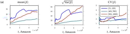
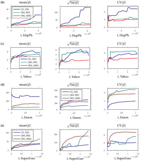
Figure 1.
Trajectories of the sample mean of the friendship index (left), their sample standard deviations (center), and their coefficients of variation (right) for three groups of nodes over the growth of the network. Nodes are grouped based on iterations at which they appear in network. These groups consist of nodes that appeared between iterations 21 and 120 (blue line), 401 and 500 (green line), and 901 and 1000 (red line). Figures present results for networks based on data of (a) user product recommendations of Amazon service, (b) HepPh citation network, (c) network of email communications within Yahoo email service, (d) Enron mail network, (e) user interactions on the SuperUser platform.
2.3. HepPh Citation Network
The next network we analyze is the co-authorship network. These networks are also called collaboration networks. The nodes of the network are authors. Between any two of them, a link is drawn if they have published a joint work. The network, abbreviated as HepPh, is a collaboration network built for authors of papers published in the journal High Energy Physics Phenomenology. When preparing the dataset, two sources were used: the archive of scientific articles, arXiv, and APOS.
The results are shown in Figure 1b. We see that the averaged trajectory of the friendship index increases for each of the three groups of nodes. The values of the sample standard deviation exceed the corresponding values of their means, which results in the values of the coefficient of variation being higher than 1.
2.4. Yahoo Email Network
Now let us consider a social network in which two users are connected if one of them sent an email to the other. The dataset we use is taken from [] and includes information about users of the Yahoo email portal. The data contain time ticks for each email sent and also include information with user IDs, which allows us to study the dynamic behavior of the network.
The results of the trajectory calculations can be found in Figure 1c. It is clearly seen that the values of the friendship index are always greater than 1 and increase for all three groups, with rare exceptions. The sample standard deviation also increases and exceeds the corresponding average values.
2.5. Enron Mail Network
In this subsection, we use a social network hosted by Enron employees. Two employees are connected by a link if one sends a corporate email message to the other. Unlike the Yahoo network, this social network has a high edge density. Another feature of the network is the disproportionately large amount of high- and extremely high-degree nodes.
However, these differences did not greatly affect the results describing the dynamic behavior of the friendship index. It can be seen in Figure 1d that the average value of this indicator is growing over time (albeit at a slow pace), and the values of the sample standard deviation exceed the corresponding average values (except for the first group of nodes). The trajectories for the coefficients of variation increase for all three groups.
2.6. Superuser Network
Let us consider another social network. We examine data about users and their interactions on the SuperUser platform. This platform allows users to ask questions about computer and technology topics, as well as to post answers. To build the network, a dataset is used that contains information about the interactions of users with the platform. The network consists of nodes representing users who are connected if one of them answered a question posted by another. In addition, a connection between users is established if one of them has posted a comment on the question or answer of another. The dataset contains time stamps of all questions and comments, which allows us to explore the dynamic behavior of the friendship index over time.
Plots of the averaged trajectories, as well as the trajectories of the sample standard deviation and the coefficient of variation, can be found in Figure 1e. We observe the growth of all trajectories for all three groups of nodes. The values of the coefficient of variation are above 1 for all groups over the entire time interval.
3. Barabási–Albert Model with Non-Linear Preferential Attachment
In this section, we examine growth-evolving networks generated using the Barabási–Albert model and its modifications. The state of a simulated network is obtained at a discreet moment of time based on the state of the network at the previous moment t. We denote as the network state at time t, with denotes as its set of nodes and denoted as the set of its links. The degree of vertex at time t is denoted as .
The Barabási–Albert model fuses two intuitive concepts: growth and preferential attachment:
- Many of the known real networks evolve based on the fact that new nodes join them. The growth of the network in the model is carried out by adding a new node to it at each discrete time. Thus, at iteration t, the network consists of t nodes. After a new node appears on the network, those vertices to which it will be attached are selected among the existing ones. The model assumes a fixed number of such nodes, and this parameter is denoted by , where .
- The choice of nodes to which a new node will be attached is carried out using the preferential attachment rule. This means that the probability of choosing a node is proportional to its degree. It is called the linear preferential attachment (LPA) mechanism. If the probability of choosing a node is proportional to its degree raised to a certain power exponent , then this rule is called the non-linear preferential attachment (NPA).
It is supposed that at initial time , consists of m vertices, , and for any .
While represents a valid nonlinear PA rule, the attachment probability grows superlinearly with the degree of a node, which leads to a phenomenon known as “winner takes all”, where a single or a few nodes monopolize most of the connections. Such networks are highly centralized, and most nodes have very low degrees, creating an extreme disparity.
Therefore, in the following, we will consider the case , since many real-world networks (such as social networks, the World Wide Web, biological networks, etc.) are better represented by models with .
Let us describe the Barabási–Albert model with the NPA mechanism in more detail. The network state at time is processed from the previous state using two steps:
- One node is added to the network; i.e., the set of vertices includes one more element: ;
- Exactly m links are attached to the newborn node; i.e., the set adds m new elements. Each of the connections appears as the result of the NPA rule application. More precisely, if is the random variable that takes the values with probabilitythen in the case of , the connection appears in the network. We perform m such independent random realizations of . Thus, .
We require the following notations:
- Denote as the node attached to the network at iteration i. Let be the degree of node at time .
- Denote as the sum of degrees for all neighbors of node at time t:
- Denote as the average degree of all neighbors of node at time t; i.e., the ratio of the entire degree of its neighbors to the degree of node taken at time t:
- Then, the friendship index of node at time t is denoted as the ratio of the average degree of all neighbors of node to its degree at moment t:
Just like real networks, synthetic networks derived from the model evolve by adding new nodes and links. Therefore, the values of local characteristics , , , and can change at each iteration. For example, if a new node joins node , then its degree will increase by 1, and the sum of the degrees of its neighbors will increase by the degree of the node attached to it; i.e., on m. Due to the use of the preferential attachment mechanism, which is probabilistic, the processes , , , and are stochastic. Moreover, since each subsequent state is determined only by the state at the moment of time preceding it, these processes are Markovian ones.
Reference [] examines the analytical properties of the friendship index in random networks generated by two models: the Barabási–Albert model and the triadic closure model by Holme and Kim []. It was proved that in the synthetic Barabási–Albert networks constructed with the linear PA mechanism, the expected values of the friendship index for node are asymptotic:
Denote
The analysis of dynamic behavior of node degree is presented in ref. [] for the Barabási–Albert networks generated using the non-linear PA mechanism (with ). It was shown that the averaged values of asymptotically behave as follows:
and the variance of follows
with some constants , and
The limit in Equation (3) exists and is unique (see []).
However, the asymptotic dynamics of are unknown for the case of non-linear preferential attachment mechanisms. In this paper, we examine the behavior of over time for the Barabási–Albert networks with the non-linear preferential attachment rule (with ). To better understand the behavior of a stochastic process over time, in this section, we will find two of its characteristics: the expected value of a random variable and its variation at time t.
We will use the following properties of the evolution of networks generated on the basis of the Barabási–Albert model with the non-linear preferential attachment vertex attachment option:
- If newborn node links to node at moment , then the degree of vertex increases from time t to by 1: . In addition, we obtain , as the degree of attached node is equal to m.
- If the newborn node links to a neighboring node of vertex at time t, then the degree of vertex does not change from time t to , , and .
4. Dynamics of
4.1. Methodology
We first describe a methodology for finding the dynamics of based on the mean-field method (Figure 2). The first step is to obtain a relation, where the left side is the increment of the quantity of interest to us between neighboring times t and , and the right side contains the sum of the products of some random variables (see , below) and the corresponding outcomes of the quantity of interest calculated using , , , and . Thus, we obtain a stochastic equation. Then, we find the mathematical conditional expectations of both parts, provided that the network is in the state. We obtain a difference equation, which we will approximate using a differential equation. We usually obtain a first-order non-homogeneous linear differential equation, the solution of which can be found using the method of variation of parameters, which will describe the dynamics of the process of interest.
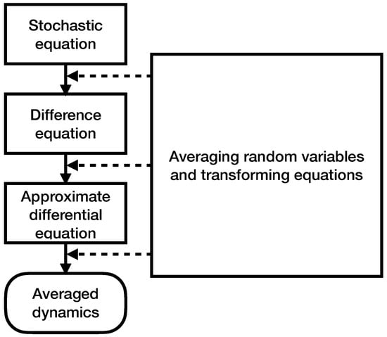
Figure 2.
The mean-field approach for evaluation of expectations and variances for .
4.2. The Expectation of
We estimate the dynamic behavior of the friendship index for node over time. First, let us find the expectation of this value at time moment t.
Let and be auxiliary random variables defined by the following:
Lemma 1.
The expected value of at iteration t follows
Proof.
Denote . We have the following difference equation:
and its approximation is as follows:
Its solution is as follows:
Since , we obtain .
Since as , we have . Then, Equation (7) can be approximated by . Its solution is . □
Lemma 2.
The expected value of at iteration t follows
Proof.
Denote . We have the following difference equation:
and its approximation is as follows:
Its solution is as follows:
Since , we obtain .
Since as , we have . Then, Equation (9) can be approximated by . It follows from as that its solution follows . □
Lemma 3.
The expected value of at iteration t follows
Proof.
Denote . The evolution of at iteration is described by the following equation:
Using , we obtain the difference equation
Then, it follows from Lemma 2 that the approximate differential equation is
Its solution is
□
It was shown in [] that . The next theorem specifies the constant c.
Theorem 1.
If , then the asymptotic expectation of the expectation for the friendship index of node at iteration t follows
Proof.
The evolution of at iteration t can be expressed as follows:
It follows from , and
that
Denote . It follows from Lemma 1 that the approximate differential equation is
the solution of which follows
□
Theorem 2.
If , then the asymptotic expectation of the quantity at the moment follows
where depends on m and γ.
Proof.
It was shown in [] that
Then, it follows from (11) that the conditional expectation of the change in the value of at iteration t can be described as follows:
Using , we obtain the following:
It was shown in [] that , and . We assume that and are independent from . Then, we obtain the following approximate first-order differential equation for :
the solution of which follows
where depends on m and . □
To study the empirical behavior of the friendship index in synthetic model-based generated networks, we use the following scheme:
- we select a node number for observation (e.g., , 50, or 100);
- we generate a large number of synthetic networks (a group of networks);
- in the process of growth of each network, we find and store the values of the friendship index for the node with the fixed number at each moment of network growth;
- we find the sample mean, the sample standard deviation, and the sample coefficient of variation for the friendship index at each point in time over the entire group of trajectories.
Following this scheme for studying the behavior of the quantities, we generate BA networks independently using the non-linear PA mechanism. The networks’ growth was restricted by 160,000 nodes. We took the number of attached links as , and we used three values of parameter . The selected parameters result in the networks being large enough to capture the dynamic behavior of the friendship index while also allowing one to experiment with the specific parameters of the model under study. The empirical values of were calculated up to 160,000. The resulting trajectories for nodes are present in the charts in the left parts of Figure 3a, Figure 3b, and Figure 3c, respectively. The choice of nodes is for visualization purposes. We can see how the values of change with the increase in the iteration at which node appears in the network.
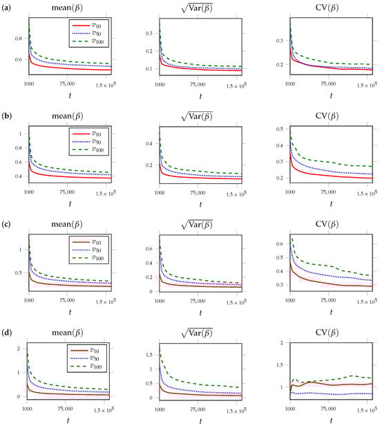
Figure 3.
Evolution of the friendship index displayed through trajectories of sample means (left), sample standard deviations (center), and sample coefficients of variation (right) for three vertices, , , found over 1000 independently simulated BA networks with non-linear PA with the following parameters: (a) , (b) , (c) , and LPA mechanism (d) . The curves in the simulation results match theoretical derivations obtained previously.
The results of this section show that in BA networks, the friendship index tends to decrease. The decrease in the friendship index in BA networks is examined and explained in more detail in ref. [].
4.3. Variance of
In this subsection, we find the asymptotic behavior for the variance of the friendship index for node with the network growth. First, we estimate the second moment of at iteration t.
Lemma 4.
If , then the second moment of at iteration t follows
Proof.
The change in the value of at iteration can be expressed as follows:
Since
we obtain the following:
Using approximation , we obtain the difference equation
Let us denote and apply Lemma 3. Then, we obtain the following approximate first-order differential equation:
the solution of which follows
□
Theorem 3.
If , then the variance of at the moment follows
Proof.
The definition of the variance implies that
Then, it follows from Lemma 4 and Theorem 1 that
□
Corollary 1.
For BA networks generated using the LPA mechanism with , the coefficient of variation for tends to a constant as :
Thus, the standard deviation of is of the same magnitude as its expectation.
Lemma 5.
For BA networks generated using the NPA mechanism with , the second moment of at iteration t follows
where depends on m and γ.
Proof.
It was shown in [] that , and . Denote . If we assume that and are independent from , then we obtain the following approximate first-order differential equation:
the solution of which follows
where depends on i, m, and . □
Theorem 4.
For BA networks with NPA, , the variance of at the moment follows
Proof.
Based on the definition of the variance, we have the following:
Then, Theorem follows from Lemma 5 and Theorem 2. □
To illustrate the behavior of the sample variance, we generate BA networks independently using the non-linear PA mechanism. The networks’ growth was restricted by 160,000 nodes. We took the number of attached links as , and we used three values of parameter . The empirical values of the sample standard deviations were calculated up to 160,000. The resulting trajectories for nodes , are present in the charts in the center parts of Figure 3a, Figure 3b, and Figure 3c, respectively.
Corollary 2.
For BA networks generatedusing they NPA mechanism with , the coefficient of variation for tends to a constant as :
Thus, the standard deviation of tends to zero with the comparable rate as its expectation.
To depict the behavior of the sample coefficient of variation, we generate BA networks independently using the non-linear PA mechanism. The networks’ growth was restricted by 160,000 nodes. We took the number of attached links as , and we used three values of parameter as well as (for the BA model with LPA). The empirical values of the sample variation coefficients were calculated up to . The resulting trajectories for for nodes are present in the charts in the right parts of Figure 3a, Figure 3b, Figure 3c, and Figure 3d, respectively. The figures clearly show that the sample standard deviations of are less than the corresponding values of their means, and the dynamics of their ratio slowly tend to zero.
5. Model with NPA and Random Numbers of Attached Links
5.1. Model Description
In the previous two sections, it was shown that the behavior of the friendship index in Barabási–Albert networks differs from its behavior in real networks. This means that the model based on the preferential attachment mechanism requires modification so that its dynamics are similar to the dynamics of the friendship index in real networks.
In this section, we use the model introduced in [], ref. [], and based on the Barabási–Albert model with the NPA mechanism that was described in Section 3, but with a random number of attached edges. In this model, the number of edges added at each iteration is a random variable taking integer values. An essential part of the model is the use of a preferential attachment mechanism in which the dependence of the probability of joining on the degree is nonlinear and obeys a power law with an exponent of .
At the initial time , the graph contains m nodes, where . At each subsequent iteration, we add one node, which means that for any , .
The state of the network in our Barabási–Albert model with the NPA mechanism and a random number of attached edges is obtained from the state of the network as follows. The algorithm adds a new node to the existing set of nodes , then generates a random number of edges , where is a non-negative integer random variable with a limited mathematical expectation and (possible infinite) variance . These edges are added to the set of edges , and each edge connects a new vertex with one of the nodes in according to the NPA rule. The NPA rule selects a node from with a probability proportional to , where is the degree of node i at time t, and is a configurable parameter.
5.2. Dynamics of
We would like to find the dynamics of the friendship index for node over time using the mean-field approach. In particular, we aimed to estimate its expectation and variance at moment .
Let and be defined as in (4) and (5). The random variable takes 1 if newborn node links to node . The random variable takes 1 if newborn node links to a neighbor of node .
Note that if the random variable takes on a value greater than the number of nodes in the network at moment t, i.e., , then we are physically unable to draw this number of edges due to the lack of the required number of nodes. Therefore, if it happens at iteration t, we generate the maximum possible number of edges; i.e., we set . We denote the random variable corrected in this way as . Denote and . It easy to see that . If , then . In the case of infinite , the value of is bounded at each moment t, while .
First, we find the expectation and the variance of the node degree at moment t. The stochastic difference equation describing the change in the degree of node at iteration is
If we take the conditional expectation of both sides at moment t, we obtain
since random variables and are mutually independent.
If , then . If , then .
5.3. Experiments and Simulation Results
Several series of experiments were conducted, during which the growth of networks was stimulated using the Barabási–Albert algorithm for different values of and . For each series of experiments with fixed algorithm parameters, 1000 graphs with 160,000 nodes were generated. During the growth of the network, every few thousand iterations, we observed the values of the friendship index of nodes that appeared in the network at steps 10, 50, and 100. For these values, the mean value, the standard deviation of the sample, and the coefficient of variation were calculated. Figures of the trajectories of these values are presented below.
We obtain the value of as the realization of a power-law-distributed random variable with exponent .
At first, we constructed networks where was set to 0.25, 0.5, and 0.75. The number of edges added at each iteration was equal to . The results are shown in Figure 4a (), Figure 4b (), and Figure 4c ().
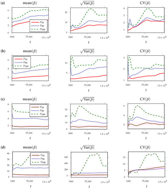
Figure 4.
Evolution of the friendship index displayed through trajectories of sample means (left), sample standard deviations (center), and sample coefficients of variation (right) for three vertices, , , found over 1000 networks independently simulated by the BA model with random numbers of attached links for t up to iterations. The networks were built using the power-law-distributed with exponent with the following parameters: (a) , (b) , (c) , (d) . The curves in the simulation results match theoretical derivations obtained previously.
Next, the graphs were constructed according to the BA model with linear PA and with a random number of edges to be joined. The results are shown in Figure 4d (with exponent and ).
In these experiments, at the beginning, the network consisted of a complete graph with five nodes. If at the next iteration, the value was greater than the number of nodes in the graph at the beginning of the iteration, then the new node was connected to all nodes in the graph.
6. Conclusions
The objective of this paper is to analyze the dynamics of the friendship index in various networks. We have obtained the expected values and variances of the friendship index in the BA networks analytically, along with the coefficient of variation.
Real networks considered in Section 2 show similar behaviors, with an increase in the expected value over time and a rapid growth in sample variance. The coefficient of variation fluctuates and remains high within a certain range. However, networks generated using the Barabási–Albert model (Section 4) exhibit a different behavior, with a decrease in the expected value over time and a decrease in variance as well, which is inconsistent with real networks.
To address this discrepancy, we examined the BA model in which the number of attached links is a random variable distributed according to the power law (Section 5). An empirical analysis showed that this modification more accurately captures the behavior of real networks. The expected values and variances for the friendship index increase, while the coefficient of variation remains volatile, but within a fixed range.
In this research, we focus only on the Barabási–Albert model. Therefore, future works may compare our findings with simulated networks obtained using other network-generating models. Moreover, other local characteristics of complex networks can be analyzed in addition to the friendship index, which is known to be limited by its dependency on the size of the network when the degree power law exponent of the network goes out of a fixed range, making it more difficult to compare networks of different sizes. Finally, more diverse real dynamic networks can be studied to obtain broader knowledge of the dynamic behavior of the local network characteristics of real-world networks.
To summarize our findings, Table 2 lists the behavioral properties of the friendship index for real networks and networks simulated using different models.
Table 2.
Comparison of networks in terms of dynamics.
Author Contributions
Conceptualization, S.S. and S.M.; methodology, S.S.; software, A.G.; validation, A.G.; formal analysis, A.G. and S.M.; resources, A.G.; data curation, A.G. and S.M.; writing—original draft preparation, A.G. and S.M.; writing—review and editing, S.S.; visualization, S.M. and A.G.; supervision, S.S.; project administration, S.S.; funding acquisition, S.S. All authors have read and agreed to the published version of the manuscript.
Funding
The work was supported by the Russian Science Foundation, project 23-21-00148.
Data Availability Statement
The original contributions presented in this study are included in the article. Further inquiries can be directed to the corresponding authors.
Conflicts of Interest
The authors declare no conflicts of interest.
References
- Siegenfeld, A.F.; Bar-Yam, Y. Introduction to Complex Systems Science and Its Applications. Complexity 2020, 2020, 6105872. [Google Scholar] [CrossRef]
- Clauset, A.; Shalizi, C.R.; Newman, M.E.J. Power-Law Distributions in Empirical Data. SIAM Rev. 2009, 51, 661–703. [Google Scholar] [CrossRef]
- De Solla Price, D. Networks of scientific papers. Science 1976, 149, 292–306. [Google Scholar]
- Klaus, A.; Yu, S.; Plenz, D. Statistical Analyses Support Power Law Distributions Found in Neuronal Avalanches. PLoS ONE 2011, 6, 1–12. [Google Scholar] [CrossRef] [PubMed]
- Newman, M.E.J. The Structure and Function of Complex Networks. SIAM Rev. 2003, 45, 167–256. [Google Scholar] [CrossRef]
- Albert, R.; Barabási, A.L. Statistical mechanics of complex networks. Rev. Mod. Phys. 2002, 74, 47–97. [Google Scholar] [CrossRef]
- Barabási, A.L.; Albert, R. Emergence of Scaling in Random Networks. Science 1999, 286, 509–512. [Google Scholar] [CrossRef]
- Piva, G.G.; Ribeiro, F.L.; Mata, A.S. Networks with growth and preferential attachment: Modelling and applications. J. Complex Netw. 2021, 9, cnab008. [Google Scholar] [CrossRef]
- Kunegis, J.; Blattner, M.; Moser, C. Preferential Attachment in Online Networks: Measurement and Explanations. In Proceedings of the 5th Annual ACM Web Science Conference, New York, NY, USA, 2–4 May 2013; WebSci ’13. pp. 205–214. [Google Scholar] [CrossRef]
- Krapivsky, P.L.; Redner, S.; Leyvraz, F. Connectivity of Growing Random Networks. Phys. Rev. Lett. 2000, 85, 4629–4632. [Google Scholar] [CrossRef]
- da Mata, A.S. Complex Networks: A Mini-review. Braz. J. Phys. 2020, 50, 658–672. [Google Scholar] [CrossRef]
- Farzaneh, A.; Coon, J.P. An information theory approach to network evolution models. J. Complex Netw. 2022, 10, cnac020. [Google Scholar] [CrossRef]
- Kashirin, V.V.; Lantseva, A.A.; Ivanov, S.V.; Kovalchuk, S.V.; Boukhanovsky, A.V. Evolutionary simulation of complex networks’ structures with specific functional properties. J. Appl. Log. 2017, 24, 39–49. [Google Scholar] [CrossRef]
- Shirzadian, P.; Antony, B.; Gattani, A.G.; Tasnina, N.; Heath, L.S. A time evolving online social network generation algorithm. Sci. Rep. 2023, 13, 2395. [Google Scholar] [CrossRef] [PubMed]
- Wu, H.; Song, C.; Ge, Y.; Ge, T. Link Prediction on Complex Networks: An Experimental Survey. Data Sci. Eng. 2022, 7, 253–278. [Google Scholar] [CrossRef]
- Turner, J.R.; Baker, R.M. Complexity Theory: An Overview with Potential Applications for the Social Sciences. Systems 2019, 7, 4. [Google Scholar] [CrossRef]
- Pal, S.; Yu, F.; Novick, Y.; Bar-Noy, A. A study on the friendship paradox–quantitative analysis and relationship with assortative mixing. Appl. Netw. Sci. 2019, 4, 71. [Google Scholar] [CrossRef]
- Feld, S.L. Why Your Friends Have More Friends Than You Do. Am. J. Sociol. 1991, 96, 1464–1477. [Google Scholar] [CrossRef]
- Eom, Y.H.; Jo, H.H. Generalized friendship paradox in complex networks: The case of scientific collaboration. Sci. Rep. 2014, 4, 4603. [Google Scholar] [CrossRef]
- Alipourfard, N.; Nettasinghe, B.; Abeliuk, A.; Krishnamurthy, V.; Lerman, K. Friendship paradox biases perceptions in directed networks. Nat. Commun. 2020, 11, 707. [Google Scholar] [CrossRef]
- Fotouhi, B.; Momeni, N.; Rabbat, M.G. Generalized Friendship Paradox: An Analytical Approach. In Social Informatics; Aiello, L.M., McFarland, D., Eds.; Springer International Publishing: Cham, Switzerland, 2015; pp. 339–352. [Google Scholar]
- Momeni, N.; Rabbat, M. Qualities and Inequalities in Online Social Networks through the Lens of the Generalized Friendship Paradox. PLoS ONE 2016, 11, e0143633. [Google Scholar] [CrossRef]
- Bollen, J.; Gonçalves, B.; van de Leemput, I.; Ruan, G. The happiness paradox: Your friends are happier than you. EPJ Data Sci. 2017, 6, 4. [Google Scholar] [CrossRef]
- Jackson, M.O. The Friendship Paradox and Systematic Biases in Perceptions and Social Norms. J. Political Econ. 2019, 127, 777–818. [Google Scholar] [CrossRef]
- Higham, D.J. Centrality-friendship paradoxes: When our friends are more important than us. J. Complex Netw. 2018, 7, 515–528. [Google Scholar] [CrossRef]
- Lee, E.; Lee, S.; Eom, Y.H.; Holme, P.; Jo, H.H. Impact of perception models on friendship paradox and opinion formation. Phys. Rev. E 2019, 99, 052302. [Google Scholar] [CrossRef] [PubMed]
- Sidorov, S.P.; Mironov, S.V.; Grigoriev, A.A. Friendship paradox in growth networks: Analytical and empirical analysis. Appl. Netw. Sci. 2021, 6, 35. [Google Scholar] [CrossRef]
- Sidorov, S.; Mironov, S.; Malinskii, I.; Kadomtsev, D. Local Degree Asymmetry for Preferential Attachment Model. In Complex Networks & Their Applications IX; Springer International Publishing: Cham, Switzerland, 2021; pp. 450–461. [Google Scholar] [CrossRef]
- Sidorov, S.; Mironov, S. Growth network models with random number of attached links. Phys. A Stat. Mech. Its Appl. 2021, 576, 126041. [Google Scholar] [CrossRef]
- Paranjape, A.; Benson, A.R.; Leskovec, J. Motifs in Temporal Networks. In Proceedings of the Tenth ACM International Conference on Web Search and Data Mining, WSDM 2017, Cambridge, UK, 6–10 February 2017; ACM: New York, NY, USA, 2017. [Google Scholar] [CrossRef]
- Holme, P.; Kim, B.J. Growing scale-free networks with tunable clustering. Phys. Rev. E 2002, 65, 026107. [Google Scholar] [CrossRef] [PubMed]
- Sidorov, S.; Mironov, S.; Grigoriev, A.; Tikhonova, S. An Investigation into the Trend Stationarity of Local Characteristics in Media and Social Networks. Systems 2022, 10, 249. [Google Scholar] [CrossRef]
- Sidorov, S.; Mironov, S.; Grigoriev, A. Measuring the variability of local characteristics in complex networks: Empirical and analytical analysis. Chaos Interdiscip. J. Nonlinear Sci. 2023, 33, 063106. [Google Scholar] [CrossRef]
Disclaimer/Publisher’s Note: The statements, opinions and data contained in all publications are solely those of the individual author(s) and contributor(s) and not of MDPI and/or the editor(s). MDPI and/or the editor(s) disclaim responsibility for any injury to people or property resulting from any ideas, methods, instructions or products referred to in the content. |
© 2024 by the authors. Licensee MDPI, Basel, Switzerland. This article is an open access article distributed under the terms and conditions of the Creative Commons Attribution (CC BY) license (https://creativecommons.org/licenses/by/4.0/).