Article

LMI-Based State Feedback Control Structure for Resolving Grid Connectivity Issues in DFIG-Based WT Systems

by
Muhammad Arif Sharafat Ali
Independent Researcher, Multan 60000, Pakistan
Eng 2021, 2(4), 562-591; https://doi.org/10.3390/eng2040036
Submission received: 24 September 2021 / Revised: 31 October 2021 / Accepted: 3 November 2021 / Published: 10 November 2021
(This article belongs to the Section Electrical and Electronic Engineering)

Abstract

:
Pertaining to the connectivity issues in wind power plants with grids, this study introduces an efficient mechanism based on a state feedback control structure to establish a fast and stable grid connection for a wind-driven doubly-fed induction generator (DFIG). Owing to a direct link through stator windings, a DFIG is significantly vulnerable to grid disturbances and experiences sizable inrush currents when connected to the power grid. The proposed control structure is designed based on a linear matrix inequality stabilization criterion, which is framed using a suitable Lyapunov candidate function. The control objective is to ensure that the stator voltage can exponentially converge to the grid voltage, accounting for balanced and unbalanced grid conditions. This is achieved by generating appropriate rotor voltage references for rotor-side converter control. This study also explores the capability of the proposed control structure to enhance the system’s robustness to external disturbances and uncertain parametric variations. Simulations confirmed the effectiveness and suitability of the developed structure in mitigating the adverse effects of the rapid onset of the grid voltage at the stator terminals of the DFIG under various grid conditions; the proposed structure could thus establish a reliable connection with negligible effects on the DFIG and the grid.

1. Introduction

1.1. Background

An increase in the share of wind energy in existing electric networks affects the dynamic behaviors of power systems. Therefore, research on safe and stable power system operations with the massive integration of wind power plants (WPPs) has garnered significant attention [1,2]. Furthermore, evolving power systems are equipped with advanced control structures to ensure reliable and quality operations [3,4,5,6]. Grid synchronization is significant for aligning highly stable system operations with wind-driven doubly-fed induction generators (DFIGs). It involves the voltage amplitude, phase angle, and frequency between the wind-turbine-generator terminal voltage and the grid voltage, with minimal deviations before establishing a connection [7,8,9]. The advantages of soft and fast grid synchronization are twofold: (1) It permits the grid connection of a DFIG with the least impact on the power system, and (2) it enables the fast reclosing of DFIGs immediately after grid faults, which is favorable in terms of providing voltage support to the grid and improving the fault ride-through capability of wind-energy conversion systems (WECSs).
In recent years, wind has been viewed as a mainstream source for generating electricity owing to the continued developments in wind turbine (WT) technology, which have made modern wind power systems more efficient and reliable. DFIGs are widely adopted solutions for variable-speed WECSs and constitute a significant fraction of the energy generated by wind power owing to reduced-rating power electronic converters [10], unlike its counterpart, which is connected to the grid through full-scale converters [11]. Despite playing a vital role in WECSs, a DFIG is susceptible to power-system transients owing to a direct grid connection through its stator windings. Consequently, whenever a DFIG attempts to establish a grid connection, large inrush currents occur, resulting in heavy stress on the electrical components of the WECS. Owing to the magnetic link between the stator and rotor windings, transient currents flow through the rotor and cause significant fluctuations in the generator torque and DC-link voltage. In addition, the rotor circuit and wind power converters (WPCs) experience these transients and further complicate the control of the DFIG.

1.2. Literature Review

Many studies have focused on the modeling, operation, and control of DFIGs [12,13,14]. Owing to their ability to independently control the active and reactive powers of the generator, field-oriented control (FOC) and vector control have been employed for DFIGs in these previous studies. Stator voltage-oriented control and stator flux-oriented control (SFOC) are two prominent types of FOC, and they exhibit the same dynamic performance. However, few published studies explain the startup and synchronization process of a DFIG-based WECS with the grid [7,8,10,15,16,17,18,19,20,21]. The authors of [7] presented an efficient control scheme for the grid synchronization of a DFIG. It used integral variable structure control to achieve direct supervision of the stator voltage. To realize a smooth grid connection, the authors of [8] proposed state feedback controllers to circumvent the drawbacks of proportional–integral (PI) controllers. The authors of [10,15] suggested grid synchronization based on the appropriate control of rotor direct and quadrature currents. However, the absence of voltage feedback resulted in substantial variations between the stator and grid voltages, which were also significantly influenced by the established grid connection. In [16], the stator voltage was directly controlled to track the grid voltage. The proposed scheme reduced computational effort. In [17], a synchronization method for DFIGs based on SFOC was presented; in this method, the stator voltage was made equal to the grid voltage by adjusting the rotor d-axis current component. By contrast, a pitch-angle controller was employed to make the frequency of the stator voltage similar to the grid voltage frequency.
The authors of [18] suggested a synchronization method in which the grid voltage is decomposed into its positive- and negative-sequence components and each one is inserted into a separate control loop to observe the unbalanced grid voltage in the stator. The initial induced voltage at the open stator terminal of a DFIG was used to synchronize with the grid voltage in [19]. An open stator negative-sequence rotor-current controller was implemented to allow the induced stator voltage to become as unbalanced as the grid voltage, allowing for a smooth connection. In [20], a new control strategy for designing the start-up procedure of a WT system equipped with DFIG was developed, in which a fuzzy logic controller was implemented to boost the system performance and reinforce the robustness under uncertain conditions. The authors of [21] proposed a direct voltage control-based synchronization technique for DFIG-based WTs.
Synchronization methods, ranging from open-loop [22,23,24] to closed-loop [25,26,27,28,29,30,31,32,33,34,35,36,37,38,39,40,41] systems, have also been proposed. The difference between these methods lies in the approach adopted for acquiring the required information from a given signal. Open-loop methods directly measure the magnitude, frequency, and phase of a given input signal. By contrast, closed-loop systems adaptively detect signal parameters via loop structures. Open-loop systems, including zero-crossing detection (ZCD), Kalman filter (KF), and discrete Fourier transform (DFT), have been proposed previously. A ZCD method to obtain grid voltage information was reported in [22]. Despite its simple implementation and robustness to frequency deviations, it suffers from several disadvantages, including poor performance under grid voltage imbalance and susceptibility to transients and noise. In [23], the authors proposed an extended KF to estimate the system frequency and phase of an input signal. Nevertheless, the complex structure and computational burden of this method were significant drawbacks. The authors of [24] suggested a recursive DFT approach for grid synchronization. This scheme was effective against distorted situations. However, it produced a phase shift with the grid voltage during DFT sampling.
Owing to their simple implementation and excellent disturbance rejection, closed-loop systems such as adaptive notch filter (ANF), delayed-signal cancellation (DSC), phase-locked loop (PLL), and frequency-locked loop (FLL) have gained more attention. An ANF-based approach for synchronization was proposed in [25,26]. Despite the excellent ability to detect symmetrical components and harmonics, this method is inherently sluggish. DSC is beneficial under grid voltage imbalance conditions. It is used for sequence separation with a fixed delay of 1/4 of a cycle [27,28]. Considering the simple implementation and accurate synchronization under various grid conditions, PLLs are applied more commonly than the other methods. Various improved PLLs, including synchronous reference frame (SRF) PLL [29,30,31,32], enhanced PLL [33], quadrature-based PLL [34], fixed-reference-frame PLL [35], and variable sampling period filter PLL [36], have been developed to cater to different grid conditions. However, their performances deteriorate during asymmetrical grid faults, as the second harmonics generated by the negative-sequence components circulate through the PLL system. In [37,38], it was reported that an FLL can estimate the input signal frequency and is reliable under variations in the frequency and voltage phase angle. However, it requires high computation efforts.
In [39], the authors proposed a novel synchronization algorithm based on a hybrid filtering technique to improve the operation of quasi-type-1 PLL under unbalanced grid voltage conditions. The authors of [40] proposed a novel FLL approach for grid synchronization that estimates the frequency and phase angle of the utility voltage in unbalanced and distorted conditions. A modified structure low-pass filter with selective harmonics filtering ability was used to enhance the disturbance rejection capability of the proposed FLL. Comprehensive research on three-phase FLLs was conducted in [41], including the FLL modeling and tuning, evaluating the benefits and drawbacks of using an in-loop filter in the FLL structure, and finally, establishing a connection between FLLs and PLLs.

1.3. Significance of Study

The aforementioned analyses indicate the practical significance of a soft and fast synchronization method for the smooth grid connection of WPPs; such a method warrants additional attention owing to its vital role in achieving system stability. Considering these circumstances, a simple and effective method covering the fundamental aspects of grid synchronization under various grid conditions was developed in this study. Based on a linear matrix inequality (LMI), efforts were directed toward developing a state feedback controller to address the stability issues caused by balanced and unbalanced grid conditions, model uncertainties, and external disturbances. Suitable control actions to improve the robustness and dynamic performance of the DFIG were conducted. The structure is insensitive to system parametric variations and suitable robustness to external disturbances. The proposed scheme was validated based on simulation studies, and the performances of the proposed and PI control schemes were compared. Finally, the control performances of both methods in tracking error were computed using some numerical indices such as integral square error (ISE), integral absolute error (IAE), integral time squared error (ITSE), and integral time absolute error (ITAE) for better judgment.

1.4. Contributions

In this study, the connectivity problems in a grid-connected WECS during the rapid onset of grid voltage under balanced and unbalanced grid conditions, parametric uncertainties, and exterior disturbances are discussed. This study contributes to the design of an LMI state feedback control structure that directly controls the stator voltage to establish a smooth and fast grid connection for a WECS, regardless of the grid conditions and with minimal impact on the system and the grid, thereby significantly improving system performance. Moreover, the advantages of this approach can be summarized as follows:
  • Based on the Lyapunov approach, voltage stabilization criteria in terms of an LMI are determined. Effective steadiness is achieved using the proposed control structure under balanced and unbalanced grid conditions, resulting in a substantial improvement in the performance of the DFIG control system.
  • The proposed method requires neither component decomposition nor a chain of cascaded current loops. Moreover, it does not request any information regarding bounds on disturbances. It only involves some basic modifications in the DFIG controls to achieve the control target. Hence, this control design is feasible and suitable for WPPs.
  • The proposed method guarantees robust system behavior unaffected by parametric uncertainties and exterior disturbances over the complete response.
  • In the event of unsuccessful fault-ride through operations, the proposed structure would establish a quick and smooth grid connection since it tracks grid voltage conditions directly. Moreover, the proposed structure would not cause any malfunctions since the stator voltage is directly regulated to match the grid voltage.
  • The proposed control scheme effectively controls stator voltages of the DFIG to reliably follow unbalanced grid voltage, frequency, and voltage phase, avoiding the impacts of inrush current to both the DFIG and the grid at the time of connection.

1.5. Paper Structure

The remainder of this paper is organized as follows. Section 2 presents the grid-connected DFIG-based WT system. Section 3 refers to the brief modeling of the DFIG. Section 4 describes the state-space modeling of the DFIG voltage dynamics. Section 5 presents the designed methodology of the proposed state feedback controller by solving an LMI condition based on a suitable Lyapunov candidate function. Section 6 justifies a closed-system stability analysis. Section 7 provides an extensive performance review of the proposed control structure with corresponding simulations. In addition, a comparative analysis with the PI control scheme is provided. Section 8 presents the conclusions of this study.

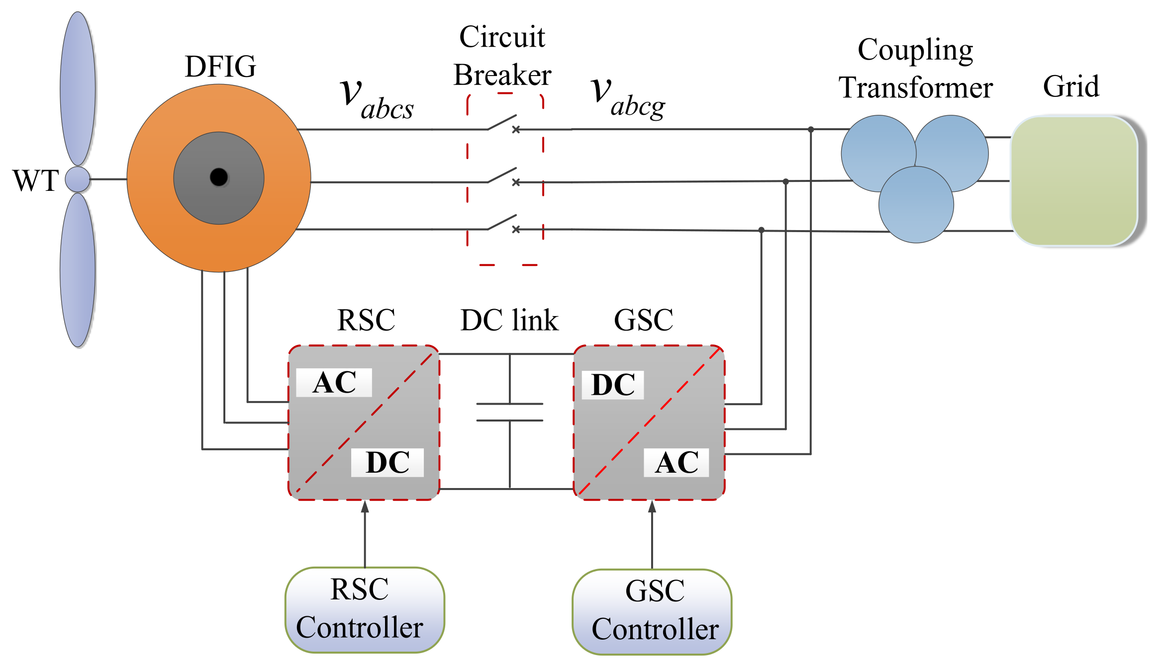
2. Overview of System Structure

For an overall perspective, a basic arrangement of a grid-connected DFIG-based WECS is presented in Figure 1. It comprises a WT, a wound rotor induction generator, and WPCs (referred to as rotor-side converter (RSC) and grid-side converter (GSC)). The stator windings of a DFIG are directly connected to a constant-frequency three-phase grid via a transformer and a circuit breaker. In contrast, the rotor windings are indirectly connected by the WPCs. The DFIG is controlled using RSC, whereas the GSC is responsible for ensuring DC-link voltage stability and the power exchange between the DC link and the grid.

3. Modeling of a DFIG

This section starts with the fundamentals of a DFIG. Here, the dynamic model of a DFIG is examined in the SRF [4,12], and the stator and rotor voltages and flux linkages are expressed as follows:
v d s = R s i d s + d ψ d s d t j ω s ψ q s
v q s = R s i q s + d ψ q s d t + j ω s ψ d s
v d r = R r i d r + d ψ d r d t j ω s l ψ q r
v q r = R r i q r + d ψ q r d t + j ω s l ψ d r
Here, vds and vqs are the direct (d) and quadrature (q) axes components of stator voltage, respectively; vdr and vqr are the dq axis components of rotor voltage, respectively; ids and iqs are the dq axis components of stator current, respectively; idr and iqr are the dq axis components of rotor current, respectively; ψds and ψqs are the dq axis components of stator-flux linkages, respectively; ψdr and ψqr are the dq axis components of rotor-flux linkages, respectively; Rs and Rr are the stator and rotor resistances, respectively; and ωs and ωsl are the electrical angular frequency and slip frequency, respectively. The dynamics of the stator- and rotor-flux linkages are written as
ψ d s = L s i d s + L m i d r
ψ q s = L s i q s + L m i q r
ψ d r = L r i d r + L m i d s
ψ q r = L r i q r + L m i q s
L s = L l s + L m L r = L l r + L m ω s l = ω s ω r
Here, Ls, Lr, and Lm are the stator, rotor, and magnetizing inductances, respectively; Lls and Llr are the stator and rotor leakage inductances, respectively; and ωr is the rotor electrical angular. At startup, the stator currents of the DFIG will be zero. First, the aim is to develop a direct voltage control by considering the relationship among the voltage vectors in the stator and rotor. Bring Equation (4a,b) into Equation (2a,b), respectively, to obtain
v d r = R r i d r + L r d i d r d t ω s l L r i q r .
v q r = R r i q r + L r d i q r d t + ω s l L r i d r .
From Equation (6a,b), the rotor current dynamics can be determined with d-axis and q-axis real component equations as
d i d r d t = 1 L r v d r R r i d r + ω s l L r i q r .
d i q r d t = 1 L r v q r R r i q r ω s l L r i d r .
Substituting Equation (3a,b) into Equation (1a,b), respectively, yields
v d s = R s i d s + L m d i d r d t ω s L m i q r .
v q s = R s i q s + L m d i q r d t + ω s L m i d r .
Considering the derivatives of Equation (8a,b), we obtain
d v d s d t = L m d 2 i d r d t 2 ω s L m d i q r d t .
d v q s d t = L m d 2 i q r d t 2 + ω s L m d i d r d t .
Furthermore, substituting Equation (7b) into Equation (9a) and Equation (7a) into Equation (9b) yields the stator-voltage dynamics in terms of the rotor currents.
d v d s d t = L m d 2 i d r d t 2 ω s L m L r v q r R r i q r ω s l L r i d r .
d v q s d t = L m d 2 i q r d t 2 + ω s L m L r v d r R r i d r + ω s l L r i q r .

4. State-Space Representation of DFIG Voltage Dynamics for Grid Connection

The proposed approach is based on state transformation and linearization, which require information the WECS parameters to be regarded. As stated, the DFIG is modeled in the SRF, and in this regard, the d-axis of the SRF is associated with the grid voltage, whereas the q-axis component will be zero.
u d g = V g ,   u q g = 0
Here, Vg represents the grid voltage magnitude; udg and uqg are the dq axis components of grid voltage, respectively. The errors between the reference and measured stator voltages are given by
ξ d = v d s v d s r e f = v d s u d g ξ q = v q s v q s r e f = v q s u q g ,   u q g = 0   .
Taking the time derivative of Equation (12) yields
d ξ d d t = d v d s d t d ξ q d t = d v q s d t .
On substituting Equation (10a,b) into Equation (13), the voltage-error dynamics can be obtained as
d ξ d d t = d v d s d t = L m d 2 i d r d t 2 + ω s ω s l L m i d r + ω s L m L r R r i q r ω s L m L r v q r
d ξ q d t = d v q s d t = L m d 2 i q r d t 2 + ω s ω s l L m i q r ω s L m L r R r i d r + ω s L m L r v d r
Combining Equation (14a,b) in a matrix form, as shown below, yields
d d t v d s v q s = L m d 2 d t 2 i d r i q r + ω s ω s l L m ω s L m L r R r ω s L m L r R r ω s ω s l L m i d r i q r + 0 ω s L m L r ω s L m L r 0 v d r v q r
There exists a time-varying parameter, i.e., the slip speed (ωsl). However, owing to the smaller time scales of electrical variables as compared to the mechanical system, Equation (14a,b) is assumed to be a set of linear systems in which the mechanical speed varies by approximately ±30% of the synchronous speed.
Before connecting to the grid, the stator current is zero; then,
i d s = 0
i q s = 0
By substituting Equation (16a,b) into Equation (1a,b), respectively, the stator-voltage equations are simplified as
v d s = d ψ d s d t ω s ψ q s
v q s = d ψ q s d t + ω s ψ d s
If the stator flux reaches steady state, the above equations can be simplified as
v d s = ω s ψ q s
v q s = ω s ψ d s
Substituting Equation (16a,b) into Equation (3a,b), respectively, we get
ψ d s = L m i d r
ψ q s = L m i q r .
By combining Equations (18a) and (19b), and Equations (18b) and (19a), the stator voltage can be represented by the rotor current.
v d s = ω s L m i q r .
v q s = ω s L m i d r .
Thus, Equation (15) can be rewritten as
d d t v d s v q s = L m d 2 d t 2 i d r i q r + R r L r ω s l ω s l R r L r v d s v q s + 0 ω s L m L r ω s L m L r 0 v d r v q r
The above expression in the state-space form can be expressed as
v ˙ s = A v s + B u + d
The first term on the right-hand side of Equation (21) is considered a disturbance (d). Here,
A = R r L r ω s l ω s l R r L r   ,   B = 0 ω s L m L r ω s L m L r 0

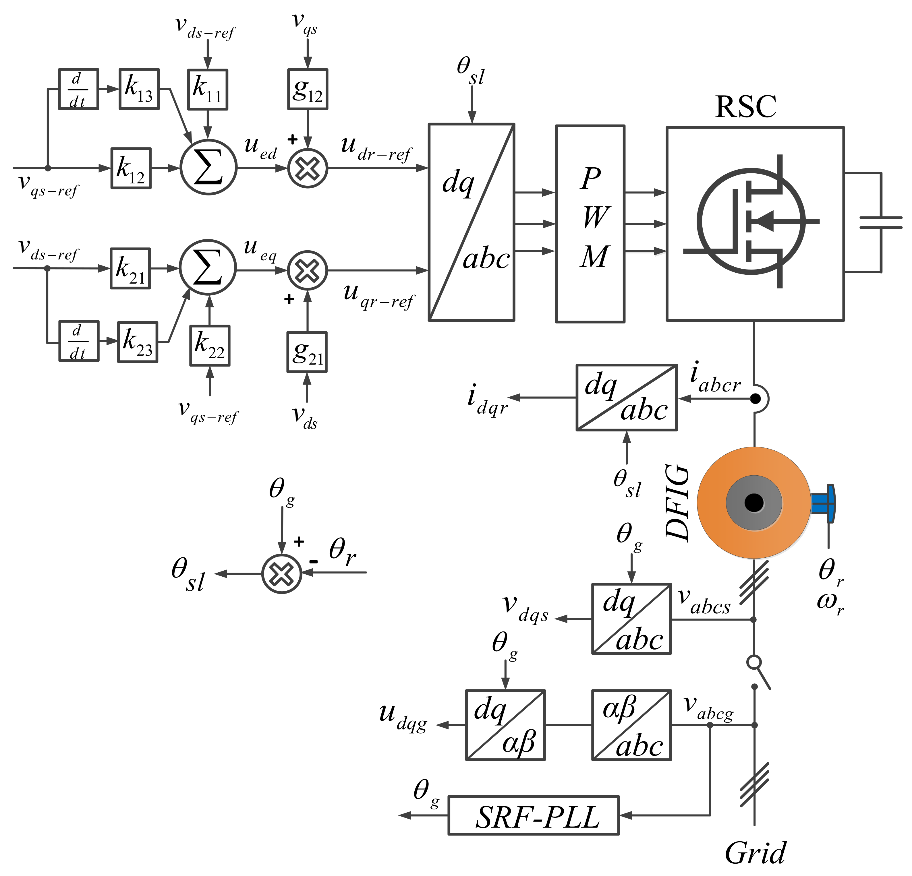
5. System Stabilization Control via LMI-Based State Feedback

Precise tracking of the grid-side voltage is achieved via introducing appropriate control actions that make the stator voltage similar to the grid voltage; this is pursued throughout the study. This section explains the design of a state feedback control structure within the LMI framework. To this end, stator voltage control is emphasized owing to its ease and practicability.
Consider a system described by
x ˙ = A x + B u
Here, x ∈ ℜn and u ∈ ℜn denote the state and system inputs, respectively. A ∈ ℜn × n and B ∈ ℜn × n are established real matrices. The objective of the state feedback is to provide the system stability by xxref, where xref is the reference signal. Prior knowledge of the following theorem and lemmas is necessary before initiating the control structure design.
Lemma 1. 
If and only if a system x ˙ = A x is exponentially stable, (a) A must be Hurwitz, which indicates that all eigenvalues of A have negative real parts, and (b) for a matrix L = LT > 0, if there is a unique positive-definite symmetric matrix W, it satisfies
W A + A T W = L
Proof. 
Define a Lyapunov candidate function as
V ( x ) = x T W x
where W is a symmetric positive-definite matrix. Taking the time derivative of V:
V ˙ ( x ) = x T W A + A T W x
If we want to ensure that the control target is achieved, then
W A + A T W < 0
Since A is Hurwitz, the above equation will be satisfied. Therefore,
V ˙ ( x ) = x T L x 0
Thus, V ˙ is negative definite if and only if L is positive definite. In other words, V and V ˙ are both positive-definite functions, and the system is exponentially stable. As a result, V exponentially converges to zero. □
Lemma 2. 
Suppose f , Y : 0 , ; then
Y ˙ η Y + f   ,     0 t 0 t
which implies that
Y ( t ) e η t t 0 Y ( t 0 ) + t 0 t e η t τ f ( τ ) d τ ,     0 t 0 t
for any finite constant η.
Proof. 
Suppose
υ ( t ) Y ˙ + η Y f
Here,
υ ( t ) 0
which implies that
Y ( t ) e η t t 0 Y ( t 0 ) + t 0 t e η t τ f ( τ ) d τ + t 0 t e η t τ υ ( τ ) d τ
Then,
Y ( t ) e η t t 0 Y ( t 0 ) + t 0 t e η t τ f ( τ ) d τ   υ ( t ) < 0   a n d     0 t 0 t
Assuming that f = 0, then
Y ˙ η Y
Integrating the above equation, we obtain
Y ( t ) e η t t 0 Y ( t 0 )
This implies that Y→0 exponentially for a positive constant η. This completes the proof.
As the precise tracking of the grid-side dq voltages is necessary, the tracking error is defined as
ε = x x r e f
Then, taking the derivative of Equation (30),
ε ˙ = A x + B u x ˙ r e f
To ensure system stability, a controller is designed as
u = G x + u e
Here, G is the state feedback gain, and it is obtained by solving an LMI.
u e = G x r e f B 1 A x r e f + B 1 x ˙ r e f
Then,
u = G x G x r e f B 1 A x r e f + B 1 x ˙ r e f = G ( x x r e f ) B 1 A x r e f + B 1 x ˙ r e f = G ε B 1 A x r e f + B 1 x ˙ r e f
and
ε ˙ = A x + B G ε B 1 A x r e f + B 1 x ˙ r e f x ˙ r e f = A x + B G ε A x r e f + x ˙ r e f x ˙ r e f = A ε + B G ε
Remark 1. 
The controller gains matrix (G) is determined by solving an LMI, which is carried out by choosing an appropriate Lyapunov candidate function.
Theorem 1. 
Consider system (21) and control law (32). If there exists a positive-definite symmetric matrix P = PT > 0, then the following LMI is satisfied:
σ P + P A + A T P + M T + M < 0
Here, σ > 0. Thus, the controller (32) guarantees the exponential stability of the system (21), and the controller gains matrix can be obtained as
G = ( P B ) 1 M

6. Closed-System Stability Analysis

A stability analysis is required to strengthen the system stability by forcing state trajectories to the equilibrium manifold after fulfilling system requirements. For this purpose, a Lyapunov candidate function is chosen as
V = ε T P ε
where P is a positive-definite symmetrical diagonal matrix. Considering the derivative of Equation (38), we obtain
σ V + V ˙ = σ V + ( ε T P ) ε + ε T P ε ˙ = σ V + ε ˙ T P ε + ε T P ε ˙ .
Substituting Equation (35) into Equation (39), we obtain
σ V + V ˙ = σ V + A ε + B G ε T P ε + ε T P A ε + B G ε = σ V + ε T ( A + B G ) T P ε + ε T P ( A + B G ) ε = σ V + ε T   A T P ε + ε T G T B T P ε + ε T P A ε + ε T P B G ε = σ V + ε T   P A + A T P + G T B T P + P B G ε = σ ε T P ε + ε T ϕ   ε = ε T   σ P + ϕ ε .
where
ϕ = P A + A T P + G T B T P + P B G
By adding Lemma 1 to Equation (40), the new inequality becomes
σ V + V ˙ ε T   L ε
As G and P are not known, we linearize Equation (41) by defining M = PBG. Using the LMI YALMIP toolbox, the values of P and M are obtained.
σ P + ϕ = σ P + P A + A T P + M T + M < 0 .
In this context,
σ V + V ˙ 0
Using Lemma 2, we get
V ( t ) V ( 0 ) exp ( σ t )
This implies that if t→∞, then V(t)→0 and ε→0. As a result, the voltage error converges to zero exponentially.
Theorem 2. 
Lyapunov Theorem for Exponential Stability
Consider a time-invariant system
x ˙ = f ( x )
where f : D N N is locally Lipschitz and x = 0 ∈ D is an equilibrium point of the system. If there exists a function V : D such that it satisfies the following conditions, then x = 0 is exponentially stable.
Proof. 
Choose a Lyapunov candidate function (38). Here,
  • V is continuously differentiable
  • V is positive-definite function
    V ( 0 ) = 0 V ( x ) > 0     x   D \ 0   i n   D =
  • The time derivative of V is negative definite
    V ˙ ( 0 ) = 0 V ˙ ( x ) < 0     x   D \ 0   i n   D =
    which was already established in Equation (44). It ensures the non-singularity of the control system (32) and the closed-system stability is guaranteed. □
Lemma 3. 
Consider the following system
x ˙ = f ( x ) ,   x ( 0 ) = x 0
where
x = x 1 , x 2 , x 3 , , x N N
If there exists a continuous positive-definite function
V ( x ) : D
such that there exists a real number n > 0 and µ∈ (0, 1) such that
V ˙ ( x ) + c V ( x ) μ   0 ,   x   \ 0
then the origin is a definite-time stable equilibrium of () and the settling time is
T ( x 0 ) 1 n ( 1 μ ) V ( x 0 ) ( 1 μ )
If = D = N , V is radically unbounded, and V ˙ < 0   o n   N \ 0 , then the origin is globally finite-time stable equilibrium of Equation (49).
Remark 2. 
The designed controller (32) ensures system (21) stabilization, and the controller gains matrix can be obtained using Equation (37). Consequently, the voltage-error dynamic reaches zero within a definite time, and the closed-loop system is exponentially stable.
Before establishing a grid connection of the DFIG, the stator voltage has to follow the grid voltage. The circuit breaker must be energized when the error between both voltages in terms of their amplitudes, frequencies, and phase angles is minimal, which is the ultimate objective of this study. The complete synchronization process is shown in Figure 2.
To obtain grid voltage angle information, an SRF-PLL is used, which can track the phase angle under unbalanced and distorted grid voltage conditions [12]. This angle information is used to obtain the stator and grid dq voltage components in the SRF. This is required to measure the slip angle (θsl), which can be used to convert the rotor current from the abc to dq reference frames. The slip angle is used to transform the outputs of the proposed control structure to three-phase rotor voltage references and is calculated as
θ s l = θ g θ r
Here, θg and θr are the grid voltage angle and rotor angle, respectively. Moreover, based on Equation (33), we obtain
u e d u e q = 0 g 12 g 21 0 v d s r e f v q s r e f 0 b 12 b 21 0 1 a 11 a 12 a 21 a 22 v d s r e f v q s r e f + 0 b 12 b 21 0 1 v ˙ d s r e f v ˙ q s r e f
Further, the aforementioned matrix can be rewritten as
u e d = k 11 v d s r e f + k 12 v q s r e f + k 13 v ˙ q s r e f
u e q = k 21 v d s r e f + k 22 v q s r e f + k 23 v ˙ d s r e f
In Equation (55a,b), k11, k12, k13, k21, k22, and k23 are constants and derived as
A = a 11 a 12 a 21 a 22   ,   B 1 = 0 b 12 b 21 0 1 = 0 k 13 k 23 0   , G = 0 g 12 g 21 0  
k 11 = k 13 a 21   ,   k 12 = ( g 12 + k 13 a 22 )
k 21 = ( g 21 + k 23 a 11 )   ,   k 22 = k 23 a 12
The values of the constants and gains are provided in Appendix A (Table A4). Dynamic control inputs for the RSC via the proposed control scheme are defined as
u d r r e f = g 12 v q s + u e d = g 12 v q s + k 11 v d s r e f + k 12 v q s r e f + k 13 v ˙ q s r e f .
u q r r e f = g 21 v d s + u e q = g 21 v d s + k 21 v d s r e f + k 22 v q s r e f + k 23 v ˙ d s r e f .
Here, udr-ref and uqr-ref are the output signals of the proposed control method in dq axes that control RSC.
Remark 3. 
In real power systems, parametric uncertainties, which are unknown time-varying quantities, are inevitable, and it is helpful to incorporate them in modeling to achieve system stability. Despite considering no such uncertainties, the proposed scheme itself has the flexibility to adapt well with an insignificant impact on system performance.

7. Results and Discussion

This section emphasizes the validity of the proposed control structure (Figure 2) using MATLAB/Simulink simulations. The nominal machine parameters are provided in Appendix A. The capability of the proposed control structure to resolve the system stabilization issue under balanced and unbalanced grid conditions was evaluated. Furthermore, for a performance comparison, the PI control method was considered. At the end, the performance of both control approaches in terms of time integral indices such as ISE, IAE, ITSE, and ITAE is compared. Appendix B contains the tuning procedure of the PI controller.

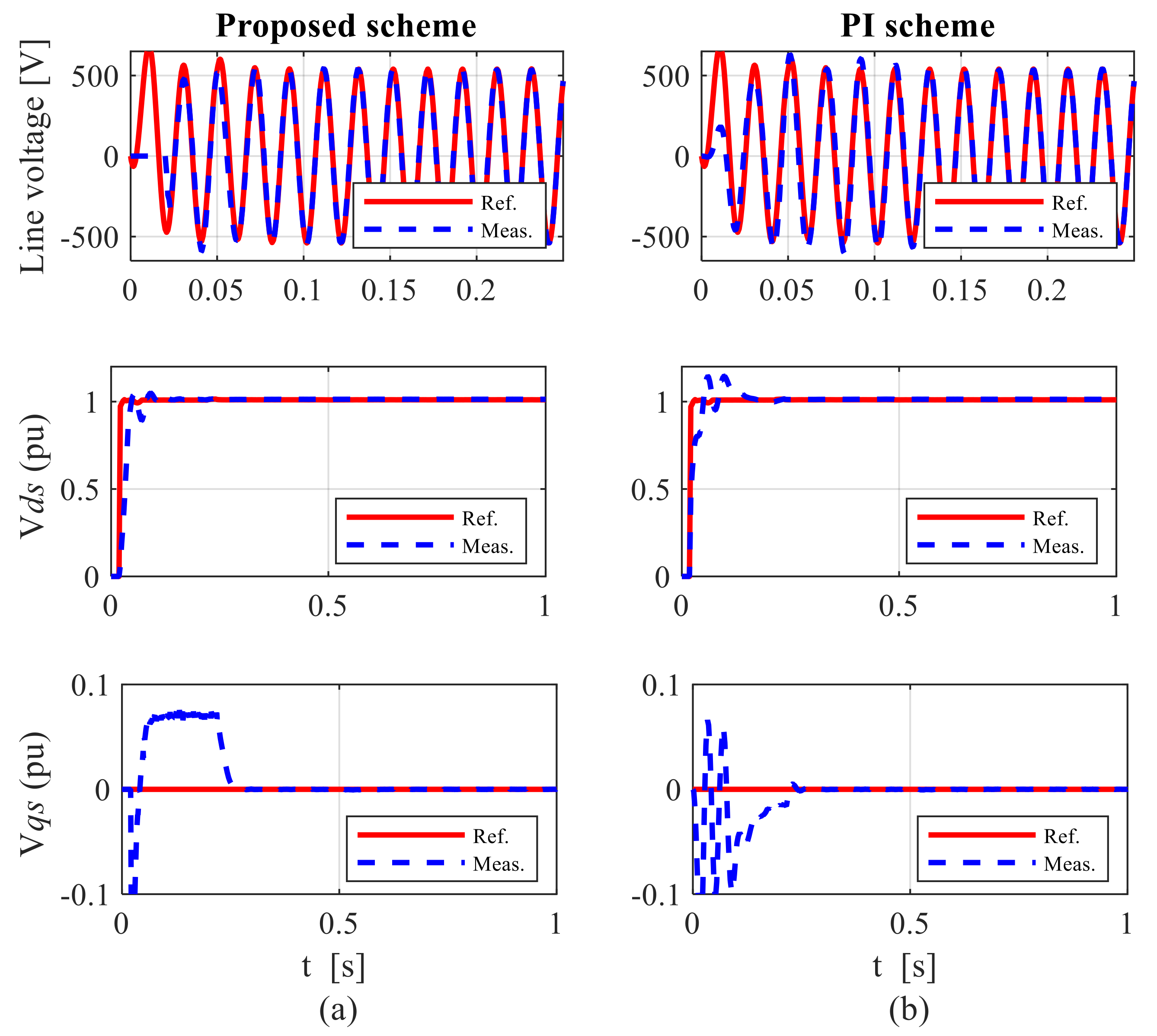
7.1. Control Performance under Balanced Grid Conditions

The control performances of the proposed and PI control methods were investigated by applying the grid voltage at 100 ms. The following cases were considered:
  • Case 1: Performance during sub-synchronous speed operation;
  • Case 2: Performance during super-synchronous speed operation;
  • Case 3: Performance under various parametric uncertainties during sub-synchronous speed operation;
  • Case 4: Performance under external disturbance during sub-synchronous speed operation.

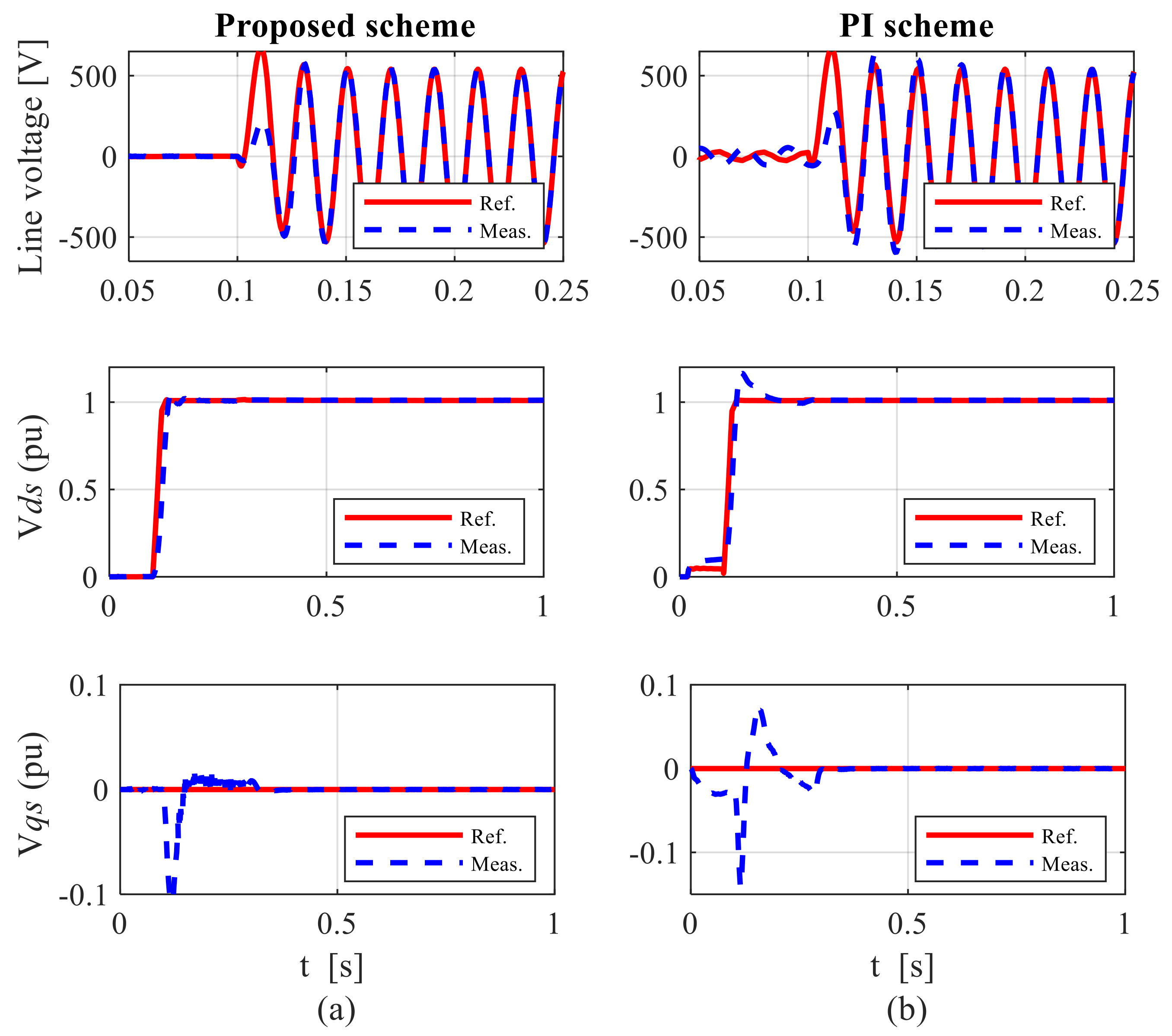
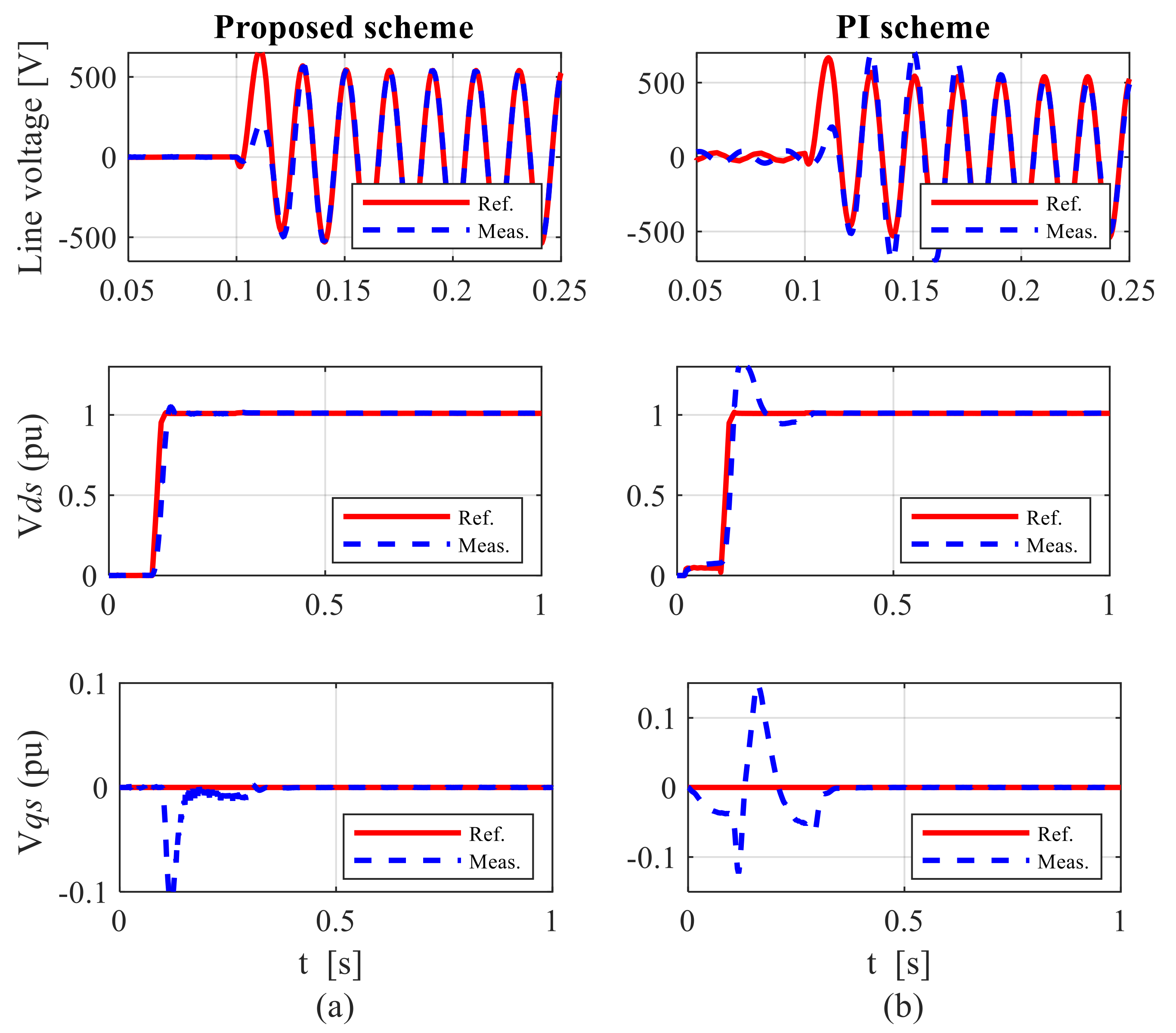
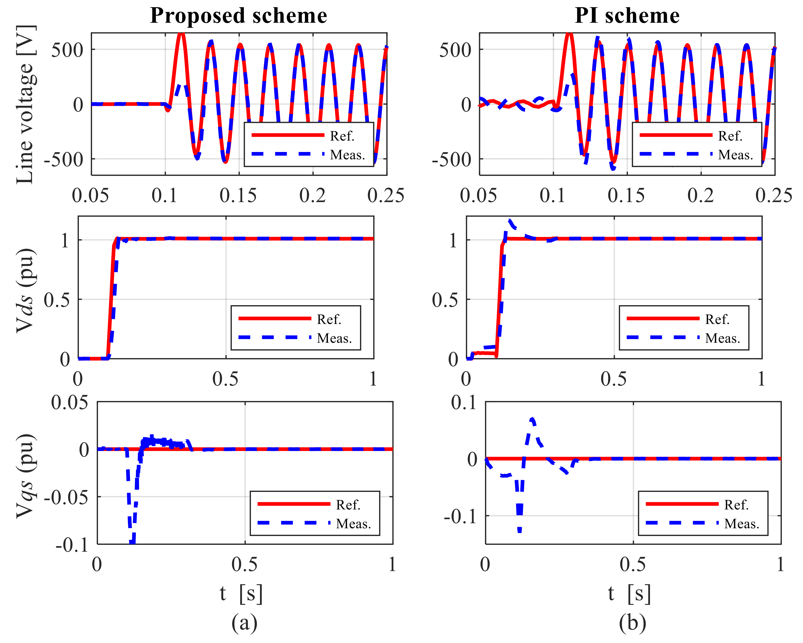
7.1.1. Case 1: Performance during Sub-Synchronous Speed Operation

Figure 3a shows the simulation results of the stator and grid voltages and their equivalent dq voltage components at sub-synchronous speed using the proposed control scheme. This figure (see Figure 3a) demonstrates that the stator voltage tracked the grid voltage quickly within one cycle. However, the d- and q-axis components of the stator voltage converged to their reference values with a fast and excellent response. The control performance of the system with the PI control method is presented in Figure 3b. The figure confirms that this method was relatively slower in tracking the grid voltage at sub-synchronous speed, as compared with the proposed method.
As seen in Figure 3b in case of the PI-based controller, the ripples were present even before the grid voltage was applied. However, the ripples were minimal with the aid of the proposed control structure, since it directly tracked grid voltage. The reason is as follows:
It is necessary to know the initial position of the rotor-speed sensor/encoder. Because of the encoder’s mechanical coupling to the rotor axis, there are two sorts of errors to account for when calculating the initial position of the rotor. The first error is generated by the encoder being mounted incorrectly, and this error must be compensated for during the synchronization procedure. The second error is the correct adjustment of the encoder. This occurs when the absolute-zero position of the rotor encoder does not match with the zero-location of the rotor windings. These errors are related to the q-axis component of stator voltage [13,15]. In terms of the performance of the proposed control scheme, it was capable of minimizing such errors; hence, two different values of q-axis stator-voltage component were noticed. Therefore, in case of the PI control method, the measured value of vqs was different from the value obtained via the proposed control method.

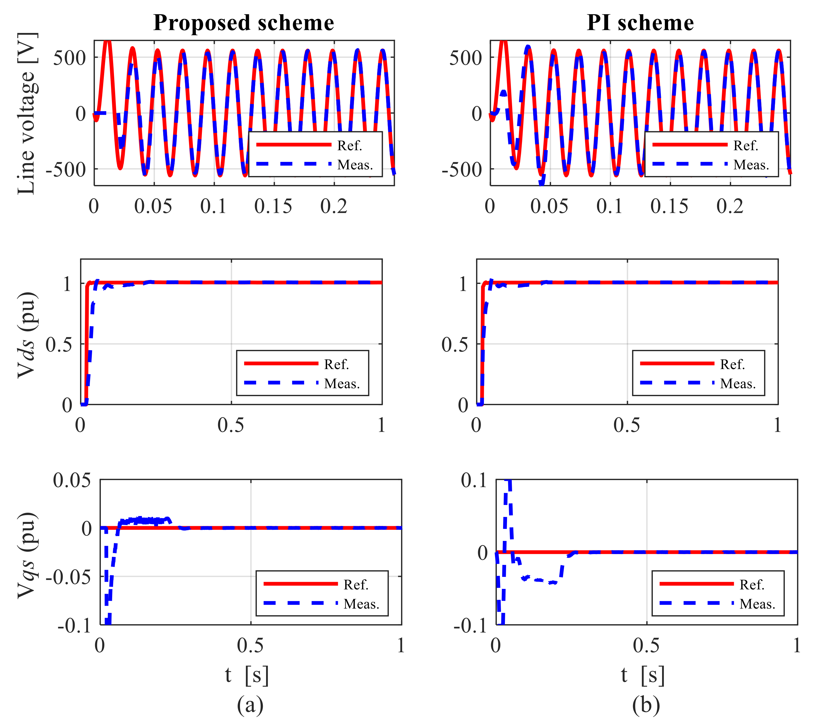
7.1.2. Case 2: Performance during Super-Synchronous Speed Operation

Figure 4 presents the simulation results of the stator and grid voltages and their equivalent dq voltage components at super-synchronous speed under both (proposed and PI) control schemes. As expected, the results were similar to those of the sub-synchronous speed operation (see Figure 3) and reflect the superior performance of the proposed control structure.

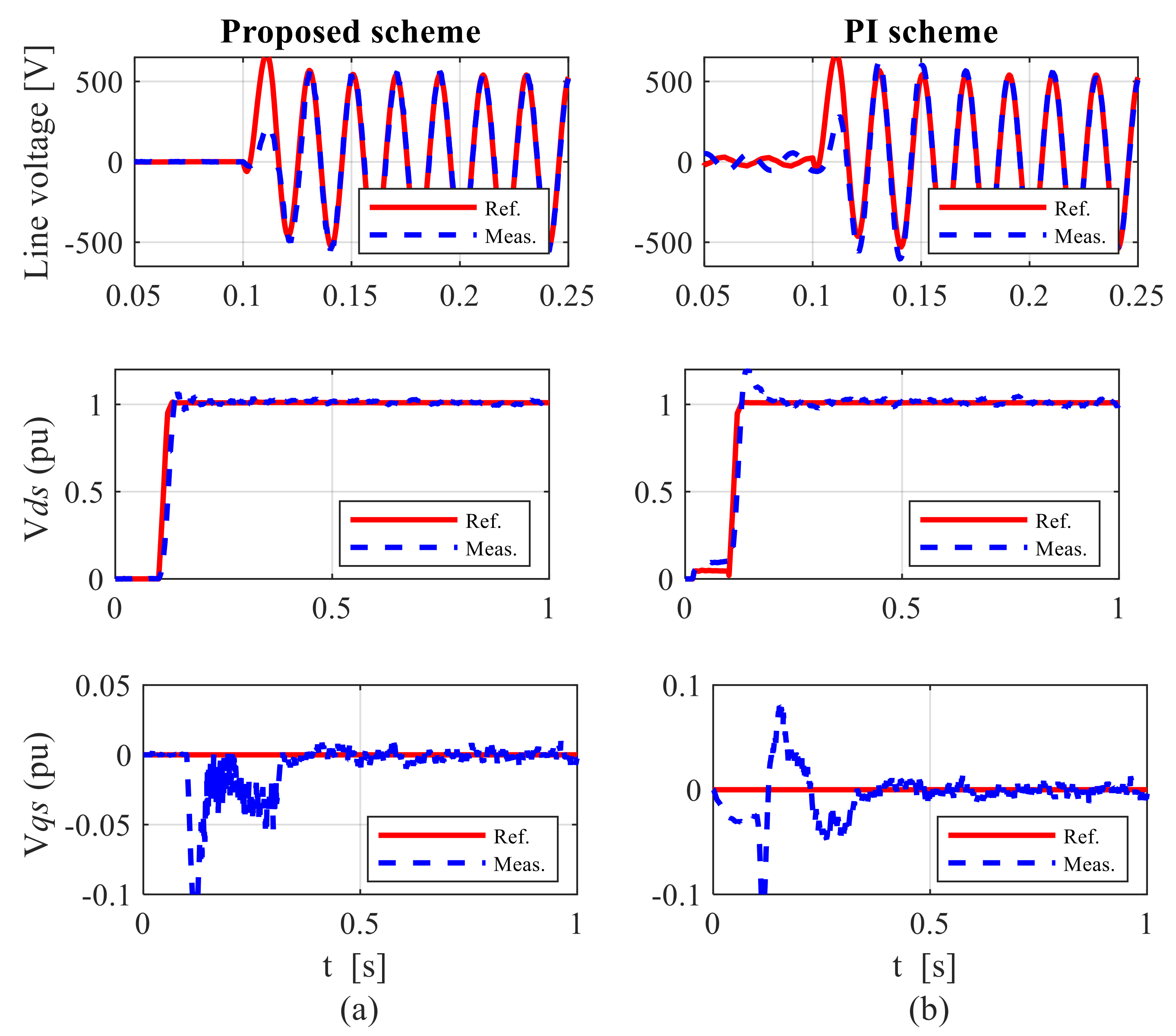
7.1.3. Case 3: Performance under Various Parametric Uncertainties during Sub-Synchronous Speed Operation

The robustness of the proposed control structure under model uncertainties in which the generator parameters are perturbed over a wide range of their rated values was investigated. In this context, the following scenarios for sub-synchronous speed operation were simulated:
  • Scenario 1: Increase the Lm of the generator to 200% of its rated value;
  • Scenario 2: Increase the Rr of the generator to 150% of its rated value;
  • Scenario 3: Decrease the Rr of the generator to 50% of its rated value.
The simulation results of the stator and grid voltages and their equivalent dq voltage components for scenarios 1–3 at sub-synchronous speed are shown in Figure 5, Figure 6 and Figure 7, respectively. When compared to the PI control, the simulation results show that the proposed control design effectively minimized voltage ripples. Despite large variations in parametric errors, the performance of the proposed control structure was admirable in delivering a significant settlement between the measured stator voltages and their references, as compared with the PI control method. As a result, unlike the PI control method, the proposed control structure was robust to machine parametric perturbations. Furthermore, the proposed design accommodated parametric uncertainties well, with almost comparable responses.

7.1.4. Case 4: Performance under External Disturbance during Super-Synchronous Speed Operation

The capabilities of both schemes against external disturbances at super-synchronous speed were investigated and compared. In this regard, white Gaussian noise (i.e., equivalent to a signal-to-noise ratio of 3 dB) was inserted into the measured stator voltage and rotor current signals. Figure 8 presents the simulation results when using the proposed and PI control schemes. The proposed method effectively suppressed noise and features enhanced functioning against external disturbances. In contrast, the results achieved with the PI control method contained relatively large-amplitude high-frequency noises.
The results of time integral indices of both control methods are presented in Table 1. Based on the above analyses, it can be inferred that the proposed control structure established a fast and smooth grid connection under balanced grid conditions and that it was robust to parametric uncertainties and external disturbances. Furthermore, the tracking performance when employing the proposed control method was superior to that when using the PI control method.

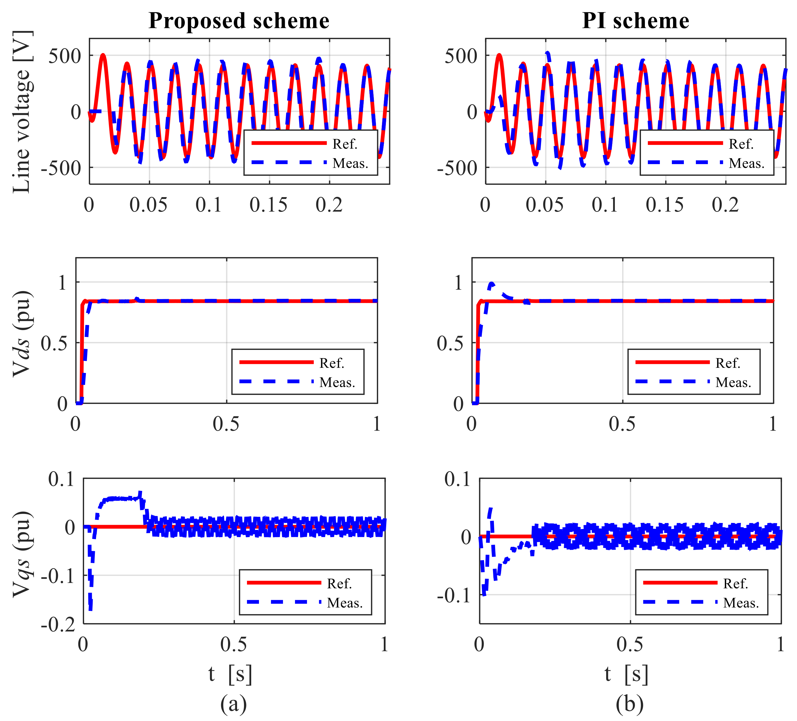
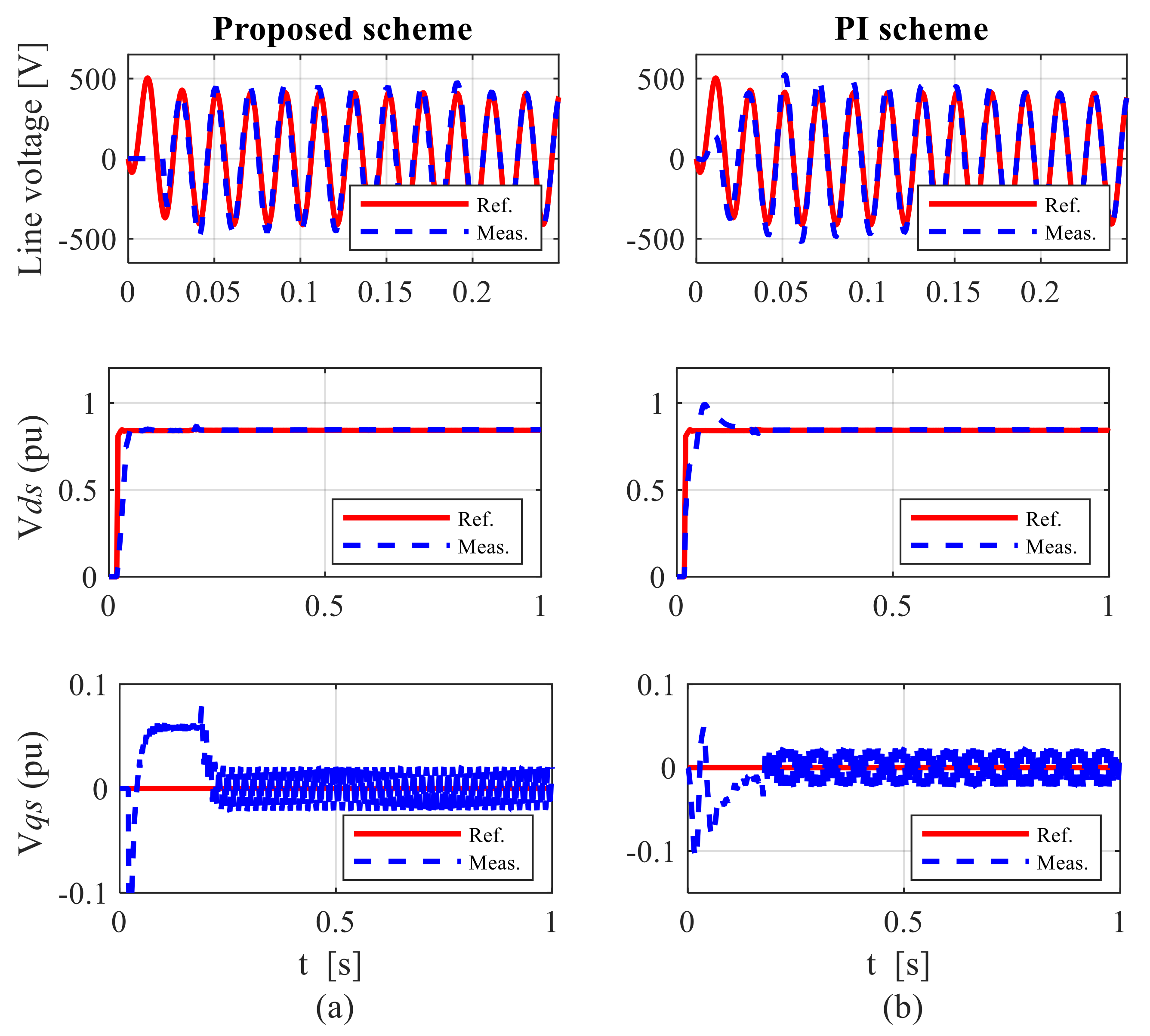
7.2. Control Performance under Unbalanced Grid Conditions

The results achieved thus far suitably indicate that the stator and grid voltages were sufficiently similar; nevertheless, it would be more beneficial to review the credibility of the proposed control structure in an uncertain environment. In this regard, the validity of the proposed control method was examined in detail by exploring the results under unbalanced grid conditions and by applying the grid voltage at t = 0 s. The following cases were considered:
  • Case 1: Performance during sub-synchronous speed operation;
  • Case 2: Performance during super-synchronous speed operation;
  • Case 3: Performance under various parametric uncertainties during super-synchronous speed operation;
  • Case 4: Performance under variation in phase angle during super-synchronous speed operation;
  • Case 5: Performance under variations in grid voltage frequency during sub-synchronous speed operation.

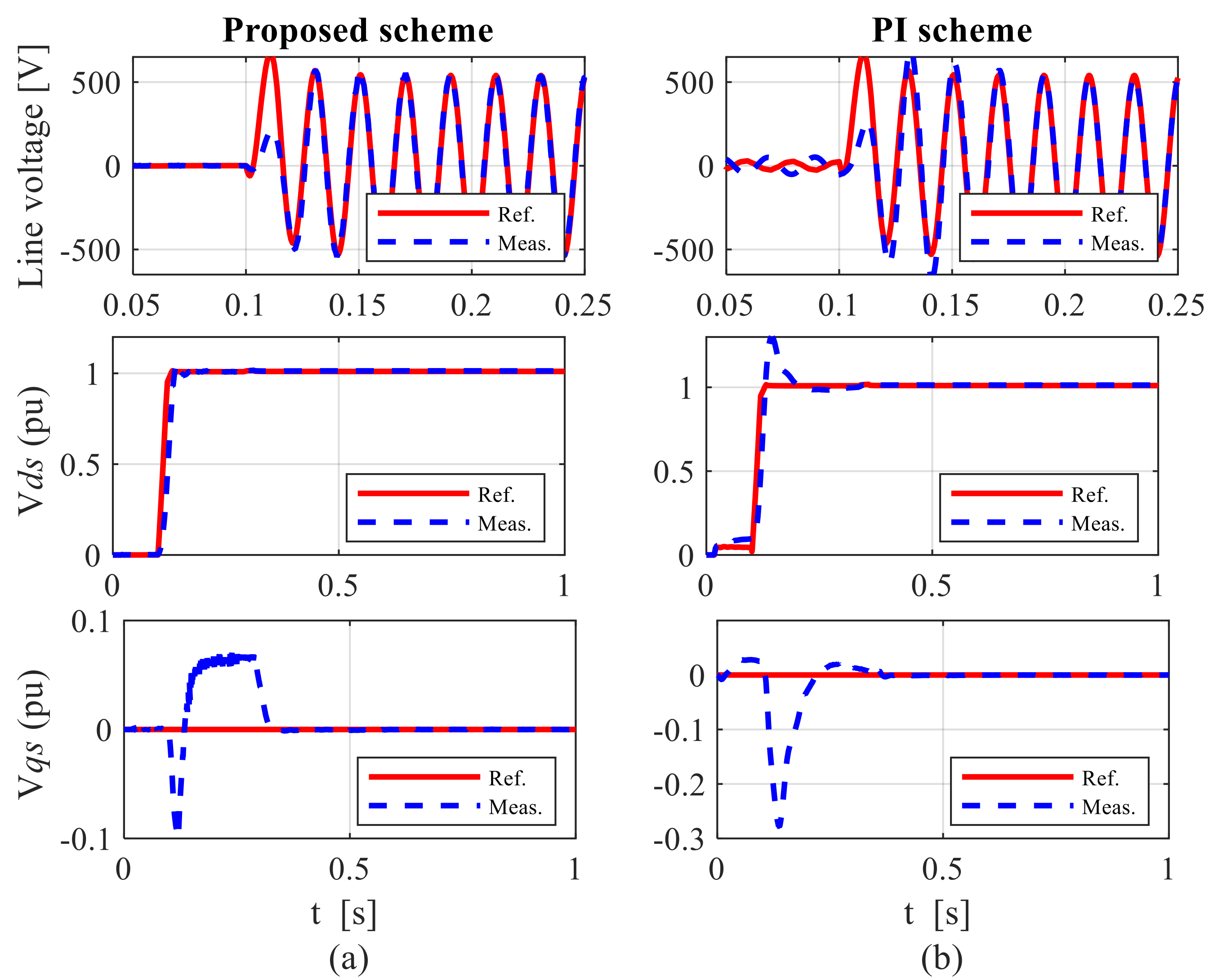
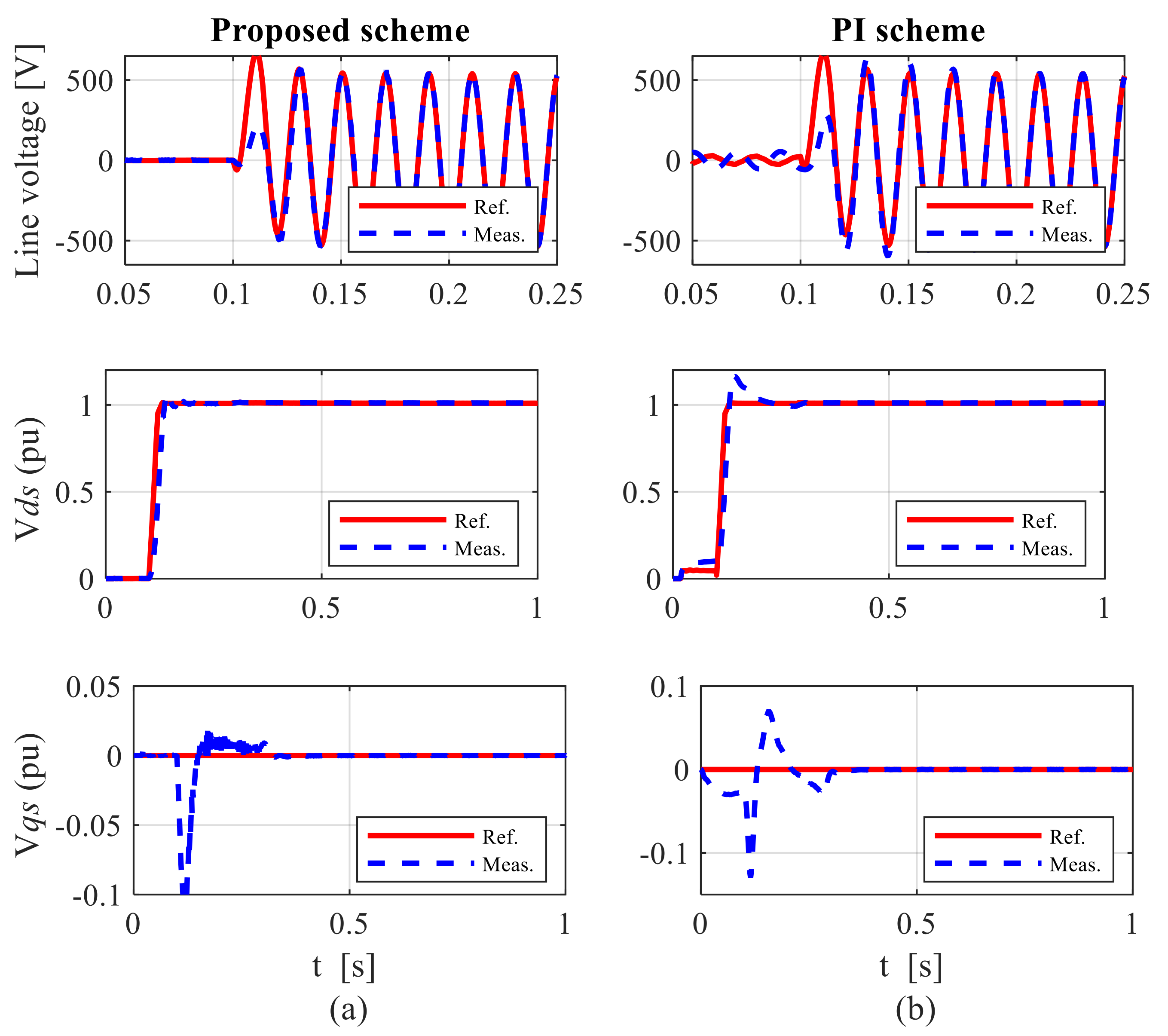
7.2.1. Case 1: Performance during Sub-Synchronous Speed Operation

In this setting, the voltage magnitudes of the two phases, i.e., Phase A and Phase B, were at their nominal values. By contrast, the magnitude of the Phase C voltage was constricted and reduced to 50% of the rated value in order to generate an unbalanced condition. Figure 9a shows the simulation results of the grid and stator voltages and their associated dq voltage components at the sub-synchronous speed achieved by means of the proposed control structure. In this figure, the stator voltage rigorously followed the grid voltage and tracked it within one cycle. The test system was simulated again with the PI control method for comparison, and the resultant waveforms are shown in Figure 9b. It was determined that the proposed structure established a precise and fast grid connection, unlike the PI control method, which required more time.

7.2.2. Case 2: Performance during Super-Synchronous Speed Operation

In this case, the voltage magnitude of Phase C was reduced to 100% of the rated value, whereas the magnitudes of the other two phases, i.e., Phase A and Phase B, were set to their nominal values. The results at the super-synchronous speed under both schemes are presented in Figure 10. As expected, similar stator voltage responses were achieved in this case as those obtained at the sub-synchronous speed, as mentioned in Section 7.2.1 (see Figure 9).

7.2.3. Case 3: Performance under Various Parametric Uncertainties during Super-Synchronous Speed Operation

The same scenarios used under the balanced grid voltage case (Section 7.1.3) were considered here to ensure the uniformity of the proposed control structure against machine parametric uncertainties. The magnitudes of the three phase voltages were similar to those at super-synchronous speed, as mentioned in Section 7.2.1. Figure 11, Figure 12 and Figure 13 refer to the responses of the stator voltages at various machine parametric variations under scenarios 1–3. The results confirm that the proposed control structure was better than the PI control scheme in the fast-tracking of the grid voltage, even under numerous perturbed machine parameters.

7.2.4. Case 4: Performance under Variation in Phase Angle during Super-Synchronous Speed Operation

Here, the magnitudes of all three phases were set to their nominal values, whereas the initial phase angles of the three phases were reduced by 20° from their nominal values. Figure 14 presents the responses of the stator voltage and their corresponding dq voltage components at super-synchronous speed under both control schemes. Based on the voltage responses, it is worth mentioning that the proposed control structure exhibited better performance in terms of the fast convergence of the stator voltage to the grid voltage under changes in the phase angles of the grid voltage.

7.2.5. Case 5: Performance under Variations in Grid Voltage Frequency during Sub-Synchronous Speed Operation

The following variations in grid frequency were applied to explore the functioning of the proposed control structure:
  • Scenario 1: Grid frequency is at 48 Hz, and all phase voltages are set to their nominal values;
  • Scenario 2: Grid frequency is at 52 Hz, and all phase voltages are set to their nominal values.
The simulation results (Figure 15 and Figure 16) show that the performance of the proposed control structure was independent of the variations in the grid voltage frequency.
Table 2 shows the results of the time integral indices for both control strategies. Thus, it can be concluded that the proposed control structure helped in the quick and precise tracking of grid voltages under balanced and unbalanced grid conditions, which is advantageous for the fast reclosing of the stator-grid contact after grid faults. Moreover, the proposed structure was robust against parametric model uncertainties and external disturbances.
The details of choosing the various types of test cases are as follows: The first two cases (Case 1 and Case 2) under balanced and unbalanced grid voltage conditions during sub-synchronous and super-synchronous speed operations, respectively, were similar. The only difference was the amplitude of the grid voltage. In Case 3, however, the authors used the same scenarios in terms of variations in machine parameters. Under balanced grid conditions, we evaluated synchronous speed operations, whereas the test system was simulated during super-synchronous speed operations under unbalanced grid conditions. Although both synchronous and super-synchronous speed operations could have been tested under balanced and unbalanced grid conditions, it would have increased the paper length.
As far as Case 4 under balanced grid conditions is concerned, it was related to the impact of external disturbance on the performances of both control methods during sub-synchronous speed operation. On the other hand, Case 4 under unbalanced grid conditions was concerned with the performance check of both approaches when the phase angle varied during super-synchronous speed operation. In relation to Case 4, the test system could have been simulated for both synchronous and super-synchronous speed operations. However, the authors believe that doing so would have lengthened the paper; therefore, we did not go over any of the possibilities. A sufficient number of test cases were simulated when evaluating the performance of their proposed control method. Since super-synchronous speed operations are more of a concern than sub-synchronous speed, the majority of the test cases under unbalanced grid conditions were attributed to super-synchronous speed operations. Case 5 was exclusively concerned with unbalanced grid conditions, in which the two scenarios in terms of variations in frequency were considered. In both scenarios, the test system was simulated for sub-synchronous speed operations.

8. Conclusions

This study focused on an important issue pertaining to the integration of WPPs, i.e., the smooth and soft grid connection of a DFIG-based WECS. Based on the Lyapunov theory, a state feedback controller was designed to cater to various grid conditions and resolve grid-coupling problems. The stability condition was stated in the configuration of an LMI. The study emphasized making the grid synchronization of WPPs as simple as possible, involving only suitable modifications for controlling the voltage at the point of common coupling. Furthermore, a comparison of time-integral performance standards such as IAE, ISE, ITSE, and ITAE was conducted, with the findings that the proposed control method outperformed the PI method. The results confirm that the control target could be achieved with good performance. The following conclusions are drawn:
  • Simulation studies showed that the proposed control structure offered fast and precise tracking of the grid voltage under various grid conditions, thus indicating its suitability in wind power applications.
  • The proposed control structure accounted well for the rapid onset of the grid voltage at the stator terminals of the DFIG under diverse grid conditions, with negligible effects on the DFIG and the grid.
  • The simple implementation of the proposed control structure makes it feasible and practical for wind energy integration.
  • The proposed control structure is independent of machine parameter variations and directly injects the desired voltage vector into the power converter.
  • It rapidly synchronizes the DFIG to the power grid, even in the presence of parametric uncertainties and exterior disturbances.
The experimental verification of the proposed control design will be the next step in this research area.

Funding

This research received no external funding.

Data Availability Statement

Not applicable.

Conflicts of Interest

The author declares no conflict of interest.

Appendix A

Table A1. Parameter of 1.5 MW WT.
ParameterValueUnit
Turbine rated mechanical power1.5MW
Rated wind speed12m/s
Air density1.225kg/m3
Optimal tip–speed ratio8.1-
Maximum power coefficient0.48-
Table A2. Parameter of 1.6 MW DFIG.
ParameterValueUnit
Rated generator power1.6MW
Pole-pair number2Nos.
Stator winding resistance2.65
Rotor winding resistance2.63
Stator leakage inductance0.1687mH
Rotor leakage inductance0.1337mH
Magnetizing inductance5.4749mH
Inertia constant3s
Friction factor0.01-
Table A3. Grid data.
ParameterValueUnit
Rated grid line-to-line voltage690V(rms)
Rated frequency50Hz
DC-link voltage reference1150V
DC-link capacitance20mF
Grid-side filter resistance1.8
Grid-side filter inductance0.5mH
Table A4. Constants and gain values.
ParameterValueParameterValue
k110.2929k125.6342
k21–5.6342k220.2929
k130.9762k23–0.9762
g12–5.6327g215.6327
Table A5. Parameters of PI controllers.
PI Gainskpki
Current controllers0.021239.938 × 10−3
Voltage controllers0.1146144

Appendix B. Tuning Procedure of PI Controllers

Bode plots were used to design the parameters of the PI controllers. A brief explanation is described here.
As shown in Figure A1, the d-axis (or q-axis) control diagram is composed of two cascaded feedback loops. In this regard, after designing the inner current loop, we can develop the controller for the outer voltage loop.
Figure A1. Control diagram of RSC with PI controllers.
Eng 02 00036 g0a1

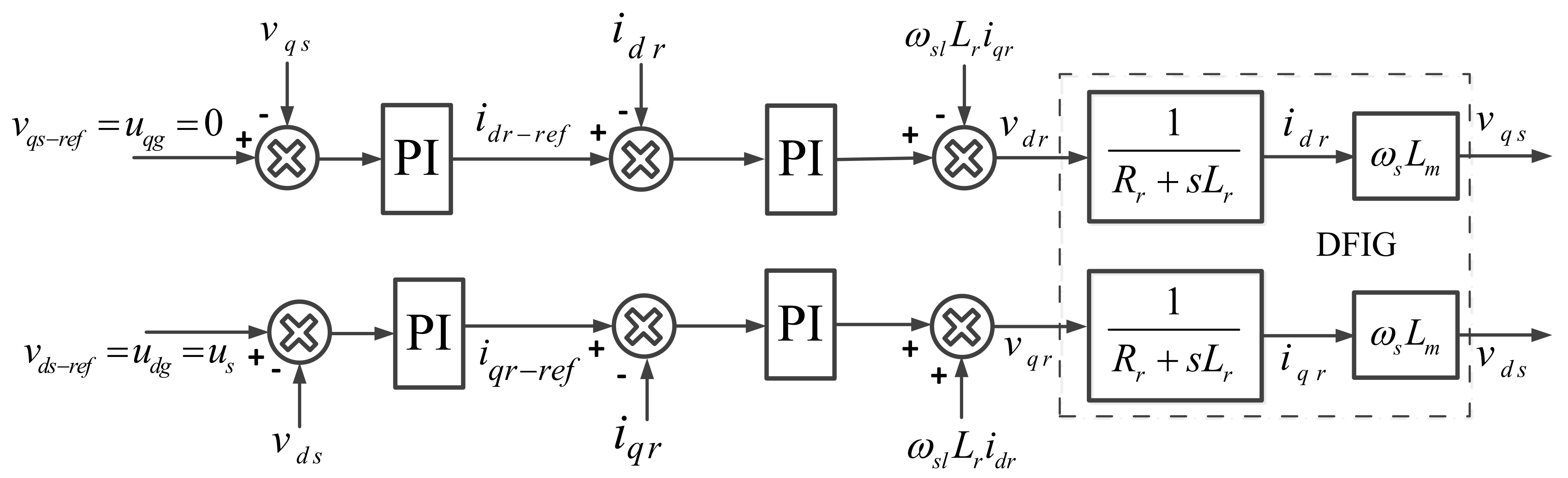
Appendix B.1. Inner-Current PI Controller Design

First, the tuning of the PI controller of the inner current-control loop is carried out. The open-loop transfer function Gvi(s) in the s-domain is expressed as
G v i ( s ) = 1 R r + s L r
It is a first-order system. Bode plots of the Gi(s) are shown in Figure A2. The crossover frequency is about 20 kHz, and its phase delay is 90°.
Figure A2. Bode plot of the open-loop transfer function Gi(s).
Eng 02 00036 g0a2
A horizontal line with an amplitude of 110 dB is a low-frequency asymptote, whereas a high-frequency asymptote is a straight line with a slope of –20 dB/decade. As illustrated in Figure A3, the intersection of these lines occurred at 0.0745 Hz.
Figure A3. Bode plot of the open-loop transfer function Gi(s) showing the asymptotes.
Eng 02 00036 g0a3
The PI regulator in the inner current control loop is
G P I i ( s ) = k p i + k i i s
The compensated open-loop function Gii(s) from the rotor-current reference to rotor current is expressed as
G i i ( s ) = G P I i ( s ) G v i ( s ) = k p i + k i i s 1 R r + s L r
The compensated open-loop transfer function has a bandwidth as wide as possible to improve the system dynamics. The crossover frequency (fc) of the compensated open-loop transfer function is set to 1/5 of the switching frequency (fs). Given that fs = 2000 Hz, fc = 400 Hz is chosen. Based on Equations (A2) and (A3), the following Equation (A4) is derived.
G i i ( s ) j 2 π f c = G P I i ( s ) G v i ( s ) j 2 π f c = 1
The corner frequency of the PI controller fi is selected to be the corner frequency of the open-loop transfer function, which is related to the zero of the PI controllers:
G P I i ( s ) j 2 π f i = k p i + k i i j 2 π f i = 0
where fi = 0.0745 Hz. Finally, the PI parameters are derived as
G i i ( j 2 π f c ) = k p i + k i i j 2 π f c 1 R r + j 2 π f c L r = 1
2 π f i = k i i k p i
The PI parameters kpi = 0.02123, kii = 9.938 × 10⁻³ are calculated. Bode plots of the compensated system Gii(s), uncompensated system Gvi(s), and PI regulator GPIi(s) are shown together in Figure A4. The crossover frequency of the compensated system is around 400 Hz, with a 90° phase margin.
Figure A4. Bode plots of the inner current-control loop design.
Eng 02 00036 g0a4

Appendix B.2. Outer-Voltage PI Controller Design

The closed-loop transfer function Hii(s) for the inner current loop is expressed as
H i i ( s ) = G i i ( s ) 1 + G i i ( s )
For the outer voltage loop, the open-loop transfer function Gii(s) from the rotor-current reference to the stator voltage can be derived as
G i v ( s ) = H i i ( s ) ω s L m
The PI controller in the outer voltage loop is given by
G P I v ( s ) = k p v + k i v s
The compensated open-loop function Gvv(s) for the outer voltage loop is described by
G v v ( s ) = G P I v ( s ) G i v ( s ) = k p v + k i v s H i i ( s ) ω s L m
To ensure the stability of the cascade control, the outer loop is deliberately designed to be far slower than the inner current loop. Here, the crossover frequency fc of the outer loop is selected to be 1/10 of the crossover frequency of the inner loop, that is, 40 Hz. Based on Equations (A10) and (A11), Equation (A12) is derived as
G v v ( s ) j 2 π f c = G P I v ( s ) G i v ( s ) j 2 π f c = 1
The PI regulator must satisfy the following equation:
G P I v ( s ) j 2 π f i = 0
From Equations (A11) and (A12), the following two equations are derived as
G v v ( j 2 π f c ) = k p v + k i v j 2 π f c H i i ( j 2 π f c ) ω s L m = 1
k p v = k i v 2 π f i
Solving the preceding two equations yields the PI parameters for the outer voltage loop, kpv = 0.1146 and kiv = 144. The parameters of the 1.6 MW DFIG test system are provided in Appendix A.
The Bode diagrams of the transfer function Giv(s), the outer PI regulator GPIv(s), and the compensated open-loop transfer function Gvv(s) are shown in Figure A5. The crossover frequency is about 40 Hz, with a phase margin of 90°.
Figure A5. Bode plots of the outer-voltage–control-loop design.
Eng 02 00036 g0a5

References

  1. Ali, M.A.S.; Mehmood, K.K.; Kim, C.-H. Full operational regimes for SPMSG-based WECS using generation of active current references. Int. J. Electr. Power Energy Syst. 2019, 112, 428–441. [Google Scholar] [CrossRef]
  2. Shen, Y.W.; Ke, D.-P.; Sun, Y.-Z.; Kirchen, D.S.; Qiao, W.; Deng, X.-T. Advanced auxiliary control of an energy storage device for transient voltage support of a doubly fed induc-tion generator. IEEE Trans. Sustain. Energy 2016, 7, 63–76. [Google Scholar] [CrossRef]
  3. Chen, J.; Lin, T.; Wen, C.; Song, Y. Design of a unified power controller for variable-speed fixed-pitch wind energy conversion system. IEEE Trans. Ind. Electron. 2016, 63, 4899–4908. [Google Scholar] [CrossRef]
  4. Ali, M.A.S.; Mehmood, K.K.; Baloch, S.; Kim, C.-H. Modified rotor-side converter control design for improving the LVRT capability of a DFIG-based WECS. Electr. Power Syst. Res. 2020, 186, 106403. [Google Scholar] [CrossRef]
  5. Ali, M.A.S.; Mehmood, K.K.; Kim, C.-H. Power System Stability Improvement through the Coordination of TCPS-based Damping Controller and Power System Stabilizer. Adv. Electr. Comput. Eng. 2017, 17, 27–36. [Google Scholar] [CrossRef]
  6. Ali, M.A.S.; Mehmood, K.K.; Park, J.K.; Kim, C.-H. Battery Energy Storage System-Based Stabilizers for Power System Oscillations Damping. J. Korean Inst. Illum. Electr. Install. Eng. 2016, 10, 75–84. [Google Scholar] [CrossRef]
  7. Chen, S.Z.; Cheung, N.C.; Wong, K.C.; Wu, J. Grid Synchronization of Doubly-fed Induction Generator Using Integral Variable Structure Control. IEEE Trans. Energy Convers. 2009, 24, 875–883. [Google Scholar] [CrossRef]
  8. Abo-Khalil, A.G.; Alghamdi, A.S.; Eltamaly, A.M.; Al-Saud, M.S.; Praveen, P.R.; Sayed, K.; Bindu, G.R.; Tlili, I. Design of State Feedback Current Controller for Fast Synchronization of DFIG in Wind Power Generation Systems. Energies 2019, 12, 2427. [Google Scholar] [CrossRef] [Green Version]
  9. Jaalam, N.; Rahim, N.; Bakar, A.; Tan, C.; Haidar, A. A comprehensive review of synchronization methods for grid-connected converters of renewable energy source. Renew. Sustain. Energy Rev. 2016, 59, 1471–1481. [Google Scholar] [CrossRef] [Green Version]
  10. Ali, M.A.S.; Mehmood, K.K.; Kim, J.S.; Kim, C.-H. ESD-based Crowbar for Mitigating DC-link Variations in a DFIG-based WECS. In Proceedings of the International Conference on Power Systems Transients, Perpignan, France, 16–20 June 2019; pp. 1–6. [Google Scholar]
  11. Ali, M.A.S.; Mehmood, K.K.; Baloch, S.; Kim, C.-H. Wind-Speed Estimation and Sensorless Control for SPMSG-Based WECS Using LMI-Based SMC. IEEE Access 2020, 8, 26524–26535. [Google Scholar] [CrossRef]
  12. Blaabjerg, F.; Xu, D.; Chen, W.; Zhu, N. Advanced Control of Doubly Fed Induction Generator for Wind Power Systems; Wiley-IEEE Press: Piscataway, NJ, USA, 2018. [Google Scholar]
  13. Abad, G.; Lopez, J.; Rodriguez, M.; Marroyo, L.; Iwanski, G. Doubly Fed Induction Machine: Modeling and Control for Wind Energy Generation; Wiley-IEEE Press: Piscataway, NJ, USA, 2011. [Google Scholar]
  14. Wu, B.; Lang, Y.; Zargari, N.; Kouro, S. Power Conversion and Control of Wind Energy Systems; Wiley-IEEE Press: Piscataway, NJ, USA, 2011. [Google Scholar]
  15. Ali, M.A.S. Utilizing Active Rotor-Current References for Smooth Grid Connection of a DFIG-Based Wind-Power System. Adv. Electr. Comput. Eng. 2020, 20, 91–98. [Google Scholar] [CrossRef]
  16. Wong, K.C.; Ho, S.L.; Cheng, K.W.E. Direct Voltage Control for Grid Synchronization of Doubly-fed Induction Generators. Electr. Power Compon. Syst. 2008, 36, 960–976. [Google Scholar] [CrossRef]
  17. Abo-Khalil, A.G. Synchronization of DFIG in wind power generation. Renew. Energy 2012, 44, 193–198. [Google Scholar]
  18. Ghasemi, A.; Refan, M.H.; Amiri, P. Enhancing the performance of grid synchronization in DFIG-based wind turbine under unbalanced grid conditions. Electr. Eng. 2020, 102, 1175–1194. [Google Scholar] [CrossRef]
  19. Khan, A.; Hu, X.M.; Khan, M.A.; Barendse, P. Doubly fed induction generator open stator synchronized control during un-balanced grid voltage condition. Energies 2020, 13, 3155. [Google Scholar] [CrossRef]
  20. Dida, A.; Merahi, F.; Mekhilef, S. New grid synchronization and power control scheme of doubly-fed induction generator based wind turbine system using fuzzy logic control. Comput. Electr. Eng. 2020, 84, 106647. [Google Scholar] [CrossRef]
  21. Muttaqi, K.M.; Hagh, M.T. A synchronization control technique for soft connection of doubly-fed induction generator based wind turbines to the power grid. In Proceedings of the 2017 IEEE Industry Applications Society Annual Meeting, Cincinnati, OH, USA, 1–5 October 2017. [Google Scholar]
  22. Perez, M.A.; Espinoza, J.R.; Moran, L.A.; Torres, M.A.; Araya, E.A. A Robust Phase-Locked Loop Algorithm to Synchronize Static-Power Converters with Polluted AC Systems. IEEE Trans. Ind. Electron. 2008, 55, 2185–2192. [Google Scholar] [CrossRef]
  23. Dash, P.; Jena, R.; Panda, G.; Routray, A. An extended complex Kalman filter for frequency measurement of distorted signals. IEEE Trans. Instrum. Meas. 2000, 49, 746–753. [Google Scholar] [CrossRef] [Green Version]
  24. McGrath, B.; Holmes, D.G.; Galloway, J.J.H.G. Power Converter Line Synchronization Using a Discrete Fourier Transform (DFT) Based on a Variable Sample Rate. IEEE Trans. Power Electron. 2005, 20, 877–884. [Google Scholar] [CrossRef]
  25. Yazdani, D.; Bakhshai, A.; Joos, G.; Mojiri, M. A Real-Time Extraction of Harmonic and Reactive Current in a Nonlinear Load for Grid-Connected Converters. IEEE Trans. Ind. Electron. 2009, 56, 2185–2189. [Google Scholar] [CrossRef]
  26. Yin, G.; Guo, L.; Li, X. An Amplitude Adaptive Notch Filter for Grid Signal Processing. IEEE Trans. Power Electron. 2013, 28, 2638–2641. [Google Scholar] [CrossRef]
  27. Wang, Y.F.; Li, Y.W. Analysis and Digital Implementation of Cascaded Delayed-Signal-Cancellation PLL. IEEE Trans. Power Electron. 2010, 26, 1067–1080. [Google Scholar] [CrossRef]
  28. Nascimento, P.S.B.; De-Souza, H.E.P.; Neves, F.A.S.; Limongi, L.R. FPGA implementation of the generalized delay signal cancelation–phase locked loop method for detecting harmonic sequence components in three-phase signals. IEEE Trans. Ind. Electron. 2013, 60, 645–658. [Google Scholar] [CrossRef]
  29. Golestan, S.; Monfared, M.; Freijedo, F.D. Design-Oriented Study of Advanced Synchronous Reference Frame Phase-Locked Loops. IEEE Trans. Power Electron. 2012, 28, 765–778. [Google Scholar] [CrossRef]
  30. Golestan, S.; Monfared, M.; Freijedo, F.D.; Guerrero, J. Advantages and Challenges of a Type-3 PLL. IEEE Trans. Power Electron. 2013, 28, 4985–4997. [Google Scholar] [CrossRef] [Green Version]
  31. Gonzalez-Espin, F.; Figueres, E.; Garcera, G. An Adaptive Synchronous-Reference-Frame Phase-Locked Loop for Power Quality Improvement in a Polluted Utility Grid. IEEE Trans. Ind. Electron. 2012, 59, 2718–2731. [Google Scholar] [CrossRef] [Green Version]
  32. Reyes, M.; Rodriguez, P.; Vazquez, S.; Luna, A.; Teodorescu, R.; Carrasco, J.M. Enhanced Decoupled Double Synchronous Reference Frame Current Controller for Unbalanced Grid-Voltage Conditions. IEEE Trans. Power Electron. 2012, 27, 3934–3943. [Google Scholar] [CrossRef]
  33. Karimi-Ghartemani, M.; Mojiri, M.; Safaee, A.; Walseth, J.A.; Khajehoddin, S.A.; Jain, P.; Bakhshai, A. A New Phase-Locked Loop System for Three-Phase Applications. IEEE Trans. Power Electron. 2013, 28, 1208–1218. [Google Scholar] [CrossRef]
  34. Liccardo, F.; Marino, P.; Raimondo, G. Robust and Fast Three-Phase PLL Tracking System. IEEE Trans. Ind. Electron. 2010, 58, 221–231. [Google Scholar] [CrossRef]
  35. Escobar, G.; Martinez-Montejano, M.F.; Valdez, A.A.; Martinez, P.R.; Hernandez-Gomez, M. Fixed-Reference-Frame Phase-Locked Loop for Grid Synchronization under Unbalanced Operation. IEEE Trans. Ind. Electron. 2010, 58, 1943–1951. [Google Scholar] [CrossRef]
  36. Carugati, I.; Donato, P.G.; Maestri, S.; Carrica, D.; Benedetti, M. Frequency Adaptive PLL for Polluted Single-Phase Grids. IEEE Trans. Power Electron. 2012, 27, 2396–2404. [Google Scholar] [CrossRef]
  37. Rodriguez, P.; Alvaro, L.; Raúl, S.M.-A.; Ion, E.-O.; Remus, T.; Frede, B. A stationary reference frame grid synchronization system for three-phase grid-connected power convert-ers under adverse grid conditions. IEEE Trans. Power Electron. 2012, 27, 99–1128. [Google Scholar] [CrossRef]
  38. Rodríguez, P.; Luna, A.; Candela, I.; Mujal, R.; Teodorescu, R.; Blaabjerg, F. Multiresonant Frequency-Locked Loop for Grid Synchronization of Power Converters under Distorted Grid Conditions. IEEE Trans. Ind. Electron. 2010, 58, 127–138. [Google Scholar] [CrossRef] [Green Version]
  39. Mellouli, M.; Mahmoud, M.; Slama, J.B.H.; Al-Haddad, K. A third-order MAF based QT1-PLL that is robust against harmon-ically distorted grid voltage with frequency deviations. IEEE Trans. Energy Convers. 2021, 36, 1600–1613. [Google Scholar] [CrossRef]
  40. Kanjiya, P.; Khadkikar, V.; El Moursi, M. A Novel Type-1 Frequency-Locked Loop for Fast Detection of Frequency and Phase with Improved Stability Margins. IEEE Trans. Power Electron. 2015, 31, 2550–2561. [Google Scholar] [CrossRef]
  41. Golestan, S.; Guerrero, J.M.; Vasquez, J.C.; Abusorrah, A.M.; Al-Turki, Y. A Study on Three-Phase FLLs. IEEE Trans. Power Electron. 2019, 34, 213–224. [Google Scholar] [CrossRef] [Green Version]
Figure 1. Basic arrangement of a grid-connected DFIG-based WECS.
Eng 02 00036 g001
Figure 2. Proposed LMI-based state feedback control structure.
Eng 02 00036 g002
Figure 3. Control performances during sub-synchronous speed operation under balanced grid conditions: (a) proposed scheme and (b) PI scheme.
Eng 02 00036 g003
Figure 4. Control performances during super-synchronous speed operation under balanced grid conditions: (a) proposed scheme and (b) PI scheme.
Eng 02 00036 g004
Figure 5. Control performances during sub-synchronous speed operation under balanced grid conditions for Lm(perturbed) = 200% Lm: (a) proposed scheme and (b) PI scheme.
Eng 02 00036 g005
Figure 6. Control performances during sub-synchronous speed operation under balanced grid conditions for Rr(perturbed) = 150% Rr: (a) proposed scheme and (b) PI scheme.
Eng 02 00036 g006
Figure 7. Control performances during sub-synchronous speed operation under balanced grid conditions for Rr(perturbed) = 50% Rr: (a) proposed scheme and (b) PI scheme.
Eng 02 00036 g007
Figure 8. Control performances during sub-synchronous speed operation under external disturbance: (a) proposed scheme and (b) PI scheme.
Eng 02 00036 g008
Figure 9. Control performances during sub-synchronous speed operation under unbalanced grid conditions: (a) proposed scheme and (b) PI scheme.
Eng 02 00036 g009
Figure 10. Control performances during super-synchronous speed operation under unbalanced grid conditions: (a) proposed scheme and (b) PI scheme.
Eng 02 00036 g010
Figure 11. Control performances during super-synchronous speed operation under unbalanced grid conditions for Lm(perturbed) = 200% Lm: (a) proposed scheme and (b) PI scheme.
Eng 02 00036 g011
Figure 12. Control performances during super-synchronous speed operation under unbalanced grid conditions for Rr(perturbed) = 150% Rr: (a) proposed scheme and (b) PI scheme.
Eng 02 00036 g012
Figure 13. Control performances during super-synchronous speed operation under unbalanced grid conditions for Rr(perturbed) = 50% Rr: (a) proposed scheme and (b) PI scheme.
Eng 02 00036 g013
Figure 14. Control performances during super-synchronous speed operation under phase-angle variation: (a) proposed scheme and (b) PI scheme.
Eng 02 00036 g014
Figure 15. Control performances during sub-synchronous speed operation for f = 48 Hz: (a) proposed scheme and (b) PI scheme.
Eng 02 00036 g015
Figure 16. Control performances during sub-synchronous speed operation for f = 52 Hz: (a) proposed scheme and (b) PI scheme.
Eng 02 00036 g016
Table 1. Control performances under balanced grid conditions. C—Case, S—Scenario.
CasesProposedPI
ISEITSEIAEITAEISEITSEIAEITAE
C_10.0049320.0009590.011040.0013540.006540.0010250.021220.002305
C_20.0050910.0008620.014750.0022260.0071690.00095430.025810.003019
C_3, S_10.0049750.00096040.011390.0014350.0081990.00093460.028150.003782
C_3, S_20.0049350.00092690.011130.0013750.0056460.0010230.021230.002308
C_3, S_30.0049310.00095140.010920.0013290.0056440.0010260.021290.002319
C_40.0051650.0010150.014560.0021850.0056640.00091010.022710.002686
Table 2. Control performances under unbalanced grid conditions. C—Case, S—Scenario.
CasesProposedPI
ISEITSEIAEITAEISEITSEIAEITAE
C_10.0052560.00024450.010480.0014620.0055840.00034180.022310.001466
C_20.011210.00041420.041120.0037040.011460.00046450.041430.003786
C_3, S_10.0073710.00021980.027710.0019850.0080030.00022640.028180.002314
C_3, S_20.0057460.00023210.023370.0015630.0083680.00036930.02950.002457
C_3, S_30.005750.00022090.023420.0015670.008380.00036970.029540.002466
C_40.007940.0002770.022550.0011580.011890.00020230.023110.00118
C_5, S_10.0092070.00011230.019090.00010950.011510.00017920.02190.0005891
C_5, S_20.0063440.0003790.019650.00081190.010520.00063460.019710.001121
Publisher’s Note: MDPI stays neutral with regard to jurisdictional claims in published maps and institutional affiliations.

