Cooperative Swarm Geometry Optimization for Assured Navigation with Range Radios in GNSS-Denied Environments ^†

Abstract

This paper addresses cooperative navigation using range radios to enable absolute positioning of low-flying UAS (LF) while operating in GNSS-denied environments. High-flying UAS (HF) are positioned above the denied area and broadcast position reports. These reports, in combination with range measurements from the LF to the HF, enable absolute positioning of the LF. (1) Methods: As the navigation performance is directly influenced by the geometry of both LF and HF’s relative positions, HF positions shall be optimized such that the Dilution of Precision (DOP) becomes minimal. The authors derive optimal azimuth angle combinations, which guarantee a minimal Horizontal Dilution of Precision (HDOP), and show the error characteristic for sub-optimal configurations, which enables the formulation of multi-vehicle-constrained optimization problems for specific combinations of numbers of HF and LF. (2) Results: An optimization problem is derived and solved for two HF aiding three LF as an example application for the derived rules. (3) Conclusions: The resulting geometry has yielded promising HDOP values, improving navigation performance in GNSS-denied environments.

1. Introduction

Unmanned Aircraft Systems (UAS) have gained much attention in many fields including infrastructure monitoring and support for emergency services. One of the most important operating environments are urban areas, where high population density and the accumulation of infrastructure requires more efficient solutions. Here, UAS—especially small UAS (sUAS)—are equipped with sensors to observe the environment and allow operators to make decisions faster. To increase efficiency and effectivity of the UAS operation, swarms of UAS can split work, e.g., to reduce the weight of individual drones by spreading the sensors over the swarm instead of equipping one drone with all required sensors.

To reduce the ground risk, which is imposed by the operation of swarms of UAS, collision avoidance is required to keep the UAS clear of obstacles and other aircrafts. Typically, to avoid collisions with the environment, tactical collision avoidance is implemented, which has widely been elaborated in the field of robotics. However, to geo-reference sensor information with the UAS’ position, UAS must be capable of estimating their absolute position reliably. In open field conditions, UAS typically rely on GNSS (Global Navigation Satellite System) as the UAS is likely to receive more than the minimum number of four Line-of-Sight (LOS) signals to the orbiting satellites to calculate an independent position estimate. In urban areas and below the elevation of the structures, an important problem is the degradation of GNSS due to shadowing, non-line-of-sight reception, and multipath [1]. Here, non-GNSS alternatives can be used to improve the reliability of the navigation solution, such as Visual Inertial Odometry (VIO) or Simultaneous Localization and Mapping (SLAM) using LiDAR scanners. In this paper, the authors build on their already proposed sensor framework, enabling UAS swarm member navigation with range radios in the absence of GNSS signals as shown in Figure 1 [2].

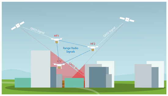
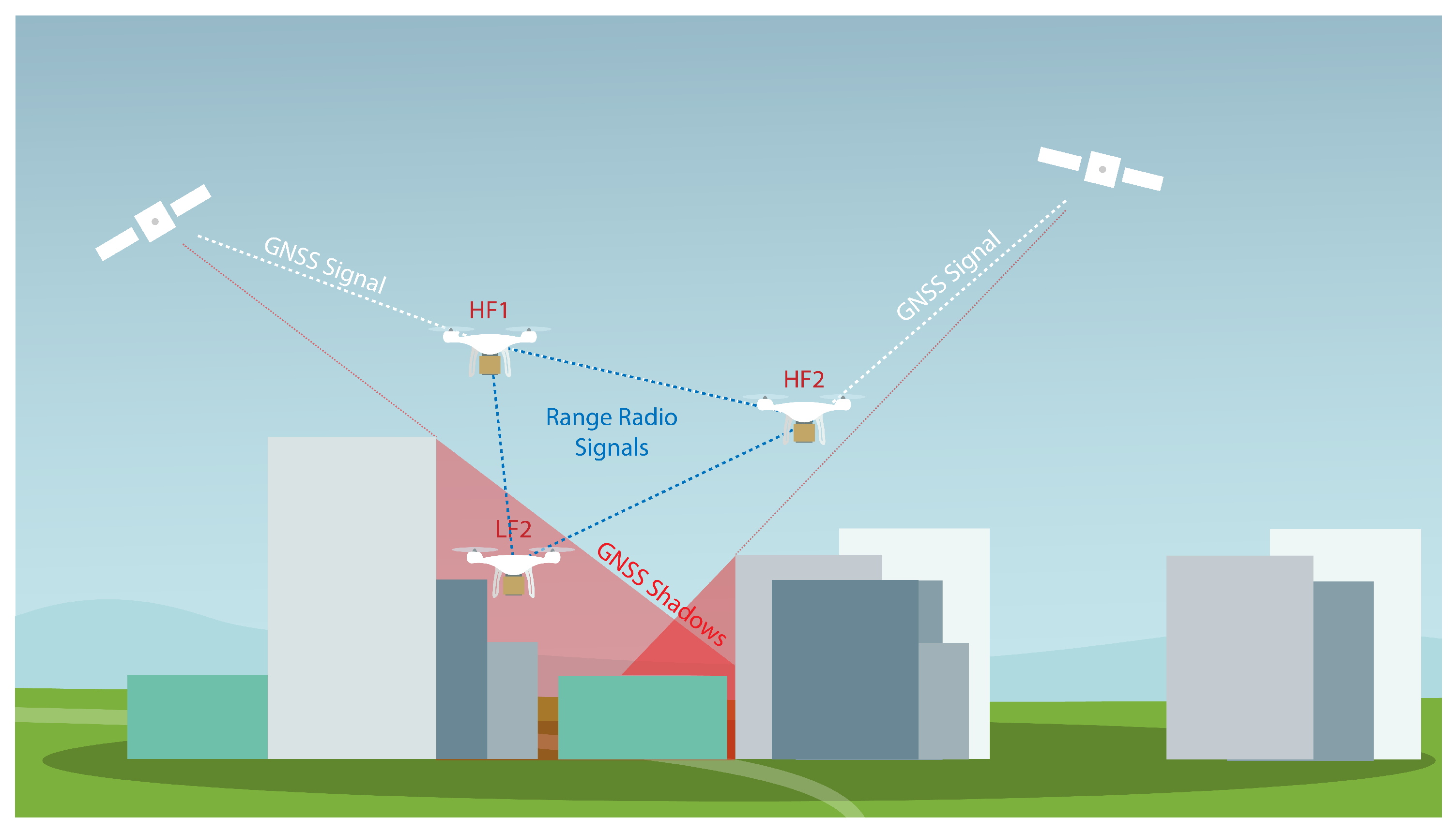
Figure 1. Swarm geometry of High Flying UAS (HF) with good GNSS reception and Low Flying UAS (LF) in a GNSS shadowed region, all connected via range radios.

The proposed scenario includes high-flying UAS (HF) equipped with GNSS receivers in open-sky conditions and low-flying UAS (LF) that perform a swarm mission close to obstacles, e.g., infrastructure monitoring; all UAS are equipped with range radios. Furthermore, the LF follow a set of swarm behavioral rules, e.g., Reynolds Rules or free operation in limited regions, while HF can move freely.

The goal of all swarm member behaviors is to simultaneously meet the mission- and navigation-performance requirements, where the latter is dependent on the geometry between the LF and HF. This paper formalizes the navigation performance of the swarm as a function of its geometry and mission parameters and finds the optimal swarm geometry while retaining Line-of-Sight (LOS) conditions between its members.

2. Methodology

2.1. Range Radio Measurements

Different techniques exist to measure the range between two transceivers. Here, we assume our lightweight swarm members to be equipped with Ultra-Wide-Band transceivers. Existing work has shown that this technology enables reliable and accurate ranging. For example, in [3], the standard deviation of Ultra-Wide-Band (UWB)-based symmetric double-sided two-way ranging (SDS-TWR) measurements was as low as 6 cm at ranges up to 5 m. This can also be seen in [4], where a ground vehicle is equipped with UWB beacons to aid the localization of a flying UAS, thus enabling relative navigation at distances of over 30 m. The standard deviation of the UWB range was found to be around 10 cm, which is at least one decade better than the uncorrected pseudorange measurement from GNSS. In the following sections and mathematical formulations, UWB range measurements are assumed to be i.i.d., specifically characterized by range noise $v_{\rho }$ that follows a bias-free normal distribution, i.e., $v_{\rho }\sim \mathcal{N}(0,{\sigma }_r^2)$.

2.2. Problem Formulation

To assess the navigation performance, the measurement equations are presented. The range ${\rho }_{i,j}$ between the unknown position of the i-th LF $p_i$ and the known position of the j-th HF $q_j$ is $h(p_i,q_j)=\left|\right|q_j-p_i{\left|\right|}_2$. For the i-th LF, the measurement vector $z_i$ is formed as a function of M HF, where $j=\{1,\dots ,M\}$:

$$z_i=\left(\begin{array}{c}{\rho }_{i,1}\\ \dots \\ {\rho }_{i,M}\end{array}\right)=\left(\begin{array}{c}h(p_i,q_0)\\ \dots \\ h(p_i,q_M)\end{array}\right)$$

(1)

To solve this equation, it is typically linearized around the current estimate. One can then solve for the position using the Least-Squares method. The linearized measurement equation is a function of the measurement matrix H, whose rows are the normalized vectors $e_{ij}$ from the HF to one LF:

$$z_i=H_i{p}_i={[e_{i1}{e}_{i2}\dots e_{iN}]}^T{p}_i.$$

(2)

In order to assess the navigation performance, one is interested in the covariance matrix of the position estimate to evaluate the accuracy:

$$\mathrm{Cov}\left(\delta x\right)=H^{+}\mathrm{Cov}\left(\delta z\right)H^{+T}$$

(3)

Here, $H^{+}$ is the pseudoinverse ${\left(H^{T}H\right)}^{-1}{H}^T$ as H is generally not invertible. As the range measurements are assumed to be independent, the covariance matrix of the range measurements $\mathrm{Cov}\left(\delta z\right)$ is assumed to be diagonal, i.e., $I{\sigma }_r^2$. For the presented measurement matrix H, it follows directly:

$$\begin{array}{cc}\hfill \mathrm{Cov}\left(\delta x\right)& =H^{+}\mathrm{Cov}\left(\delta z\right)H^{+T}\hfill \end{array}$$

(4)

$$\begin{array}{cc}\hfill & ={\left(H^{T}H\right)}^{-1}{H}^T\mathrm{Cov}\left(\delta z\right){\left({\left(H^{T}H\right)}^{-1}{H}^T\right)}^T\hfill \end{array}$$

(5)

$$\begin{array}{cc}\hfill & ={\left(H^{T}H\right)}^{-1}{H}^{T}I{\sigma }_r^{2}H{\left(H^{T}H\right)}^{-1}\hfill \end{array}$$

(6)

$$\begin{array}{cc}\hfill & ={\left(H^{T}H\right)}^{-1}{H}^{T}H{\left(H^{T}H\right)}^{-1}{\sigma }_r^2\hfill \end{array}$$

(7)

$$\begin{array}{cc}\hfill & ={\left(H^{T}H\right)}^{-1}{\sigma }_r^2\hfill \end{array}$$

(8)

$$\begin{array}{cc}\hfill & =G{\sigma }_r^2\hfill \end{array}$$

(9)

The covariance of the position estimate, and hence the navigation accuracy, is dependent on the range measurement accuracy ${\sigma }_r$ in $\delta z$ and the geometry of the ranging partners to the LF, which is captured via G. As G is dependent on H, which is formed using the geometry of the HF to the LF as shown in Equation (2), G is also referred to as the geometry matrix.

As a quality metric, the Dilution of Precision (DOP) is calculated to characterize the effect of errors in the range domain on the position estimate as a function of the geometry. For example, the Horizontal Dilution of Precision is calculated as

$$\mathrm{HDOP}=\sqrt{G_{1,1}+G_{2,2}}.$$

(10)

As initially assumed, all UWB measurements ${\rho }_{i,j}$ are i.i.d and stationary; thus, the navigation accuracy can only be maximized by optimizing the geometry of the HF positions relative to the LF positions. The optimization of geometry is a well-known research field within the domain of optimal satellite selection for GNSS positioning. For example, in [5], the authors found the relation between minimizing GDOP and maximizing the determinant of $H^{T}H$, which is related to the volume of the resulting polytope. However, in [6], the authors conclude that with an increasing number of ranging sources, the correlation between GDOP and volume decreases significantly. An additional constraint should be added as satellites closer to the regular polyhedron should be favored.

Unlike the GNSS satellite selection problem, here the satellite position, i.e., the HF position, is not given, but the optimization variable is. For UAS applications, most related work concentrates on the optimal positioning of UWB ground beacons. For example, in [7], denied environments are explored with fixed ground stations whose configuration is chosen manually. To investigate the optimal positioning of ranging sources, this paper relies on a couple of assumptions. First, the vertical position can be estimated, in addition to a GNSS- and range-radio-based estimation, with LiDAR scanners, laser altimeters, and baro-altimeters. Thus, for further optimization, the optimization goal is restricted to the horizontal 2D plane; therefore, the problem reduces to a minimization of $\mathrm{HDOP}$. Furthermore, the HF should be as low as possible to increase the observability of the LF position within the horizontal plane. Given this assumption, UAS positions are also restricted to the 2D plane, i.e., $r\in {\mathbb{R}}^{2x1}$. As LF operate close to obstacles, e.g., facades of buildings, the HF need to be positioned within an azimuth range of $\sim {180}^{\circ }$, which further reduces the region of feasible HF locations.

2.3. Single Low-Flier Optimization

Before covering the problem of optimizing the geometry of multiple LF, the optimal positioning of HF for a single LF is derived. As shown in Equation (2), the H-matrix consists of unit-length vectors from the HF to the LF, i.e., polar coordinates with an azimuth $\theta$ and a range of 1.

As H is real valued, it can be decomposed into $H=U\Sigma V^T$ using the Singular Value Decomposition, where $\Sigma$ is a diagonal matrix containing the singular values and $V^T$ contains the related right-singular vectors. As $H^{T}H$ can be decomposed into $V{\Sigma }^2{V}^T$, the geometry matrix can be rewritten as

$$\begin{array}{cc}\hfill G& ={\left(H^{T}H\right)}^{-1}\hfill \end{array}$$

(11)

$$\begin{array}{cc}\hfill & ={\left(V{\Sigma }^2{V}^T\right)}^{-1}\hfill \end{array}$$

(12)

$$\begin{array}{cc}\hfill & =V^{-T}{\Sigma }^{-2}{V}^{-1}\hfill \end{array}$$

(13)

$$\begin{array}{cc}\hfill & =V{\Sigma }^{-2}{V}^T.\hfill \end{array}$$

(14)

Here, it is used that V and U are unitary matrices, i.e., $V^T=V^{-1}$. The geometry matrix can therefore be interpreted as a Gram matrix, whose diagonal entries $G_{ii}$ are formed of $<v_i,1/s_i^2{v}_i>$. The squared HDOP can therefore be rewritten as

$$\begin{array}{cc}\hfill HDO{P}^2& =\sum _{i=1}^2\frac{1}{s_i^2}{v}_i^T{v}_i\hfill \end{array}$$

(15)

$$\begin{array}{cc}\hfill & =\frac{1}{s_1^2}+\frac{1}{s_2^2}.\hfill \end{array}$$

(16)

For M to be linearly independent unit-length vectors in H, the rank of $H^{T}H$ is assumed to be M. As the squared sum of singular values is equal to the the trace of $H^{T}H$, the squared singular values sum up to M: $s_1^2+s_2^2=M$. To minimize HDOP, ${\mathrm{HDOP}}^2$ shall be minimized, which results in the following minimization problem:

$$\begin{array}{cc}\hfill \underset{s_1,s_2}{min}{\mathrm{HDOP}}^2=& \frac{1}{s_1^2}+\frac{1}{s_2^2}\hfill \\ \hfill =& \frac{M}{s_1^2(M-s_1^2)}\hfill \end{array}$$

(17)

The function can be minimized by maximizing $s_1^2(M-s_1^2)$, which yields $s_1=\sqrt{M/2}$, and most importantly, $s_1=s_2$. This means the HDOP minimization problem can be thought of as the problem to distribute the HF directions, such that the covariance ellipse of $H^{T}H$ becomes a circle. Then, the major axis equals the minor axis and the largest singular and the smallest singular value are identical, which minimizes the HDOP.

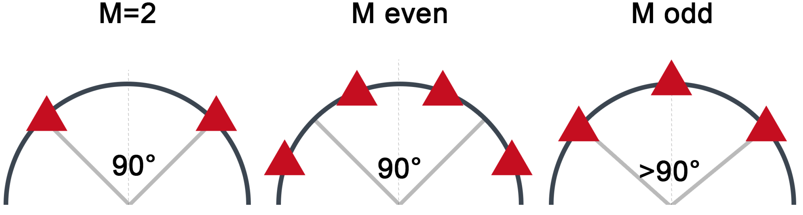
For two HF, the problem of HF positioning is trivial as the HF should be positioned such that they form an orthogonal basis. The angle between two HF and an LF should therefore be 90 degrees to maximize the HDOP for that LF.

For the number of HF being larger than two and even, pairs of HF can be symmetrically and evenly distributed around the ${\theta }_{opt}=\{-{45}^{\circ },{45}^{\circ }\}$ directions, which also directly follows from the symmetry conditions. An overview is given in Figure 2.

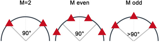
Figure 2. In 2D, optimal Horizontal Dilution of Precision (HDOP) is achieved depending on the number of HF, M; for M being even, the HF can be located at or symmetrically around an orthogonal basis; for M being odd, the optimal azimuth is a function of M.

For an odd number of HF, one HF is placed at the symmetry line between the two circle’s quarters. It can be seen that for $\theta \in [0^{\circ },{180}^{\circ }]$ one right-singular value will point towards this direction. Assuming this direction to be the y-axis and the orthogonal axis to be the x-axis, the problem can be formalized as

$$\mathrm{E}\left[{(X-{\mu }_X)}^2\right]=\mathrm{Var}\left(X\right)\stackrel{!}{=}\mathrm{Var}\left(Y\right)=\mathrm{E}\left[{(Y-{\mu }_Y)}^2\right]$$

(18)

As all vectors are centered, the mean value $\mu$ is zero. Transforming the equation to polar coordinates and using that, the radius equals to one, and the equation becomes

$$\sum _{i=1}^M\sin {\left({\theta }_i\right)}^2=\frac{M}{2}$$

(19)

Applying the knowledge that one HF is located on the symmetry axis, i.e., $x=\theta =0$, Equation (20) shows the optimal azimuth angle $\theta$ (angle between the mirror axis and the HF) for M being odd:

$${\theta }_{opt}={\sin }^{-1}\left(\sqrt{\frac{M}{2(M-1)}}\right)$$

(20)

For 3 HF, i.e., $M=3$, the optimal azimuth angle between the symmetrically chosen HF and the one on the symmetry line is $60°$, for $M=5$${\theta }_{opt}$ is $52.2°$.

The LF operate close to obstacles. Especially when flying around corners, the feasible area for the HF positioning decreases as it is essential to keep the Line-of-Sight condition between the HF and all LF. Being at orthogonal sides of a building, the overlapping area, and thus, the feasible area for HF positions, is half the size as before. To asses the effect of obstacles reducing the possible azimuth range, a Monte Carlo simulation was conducted for $M=2$ HF. The feasible $\theta$ range was restricted from ${10}^{\circ }$ to ${110}^{\circ }$. For each scenario, one million uniformly distributed independent position combinations were generated for the two HF. The combination with the best HDOP was saved and is shown in Figure 3 as a function of the maximum allowable azimuth. It can be seen that for smaller azimuth ranges, the problem tends to become more singular, resulting in an increase in HDOP. For ranges greater than ${90}^{\circ }$, two vectors can always be found, which are an orthonormal basis for the LF. For two HF, this is also the optimal condition, which means the HDOP is $\sqrt{2}$.

Figure 3. Influence of the maximum allowed azimuth range on the HDOP for two HF; towards zero, the problem tends to become singular, while for the range being greater than ${90}^{\circ }$, two vectors can always be found, which are an orthonormal basis for the LF.

2.4. Multi-User Optimization

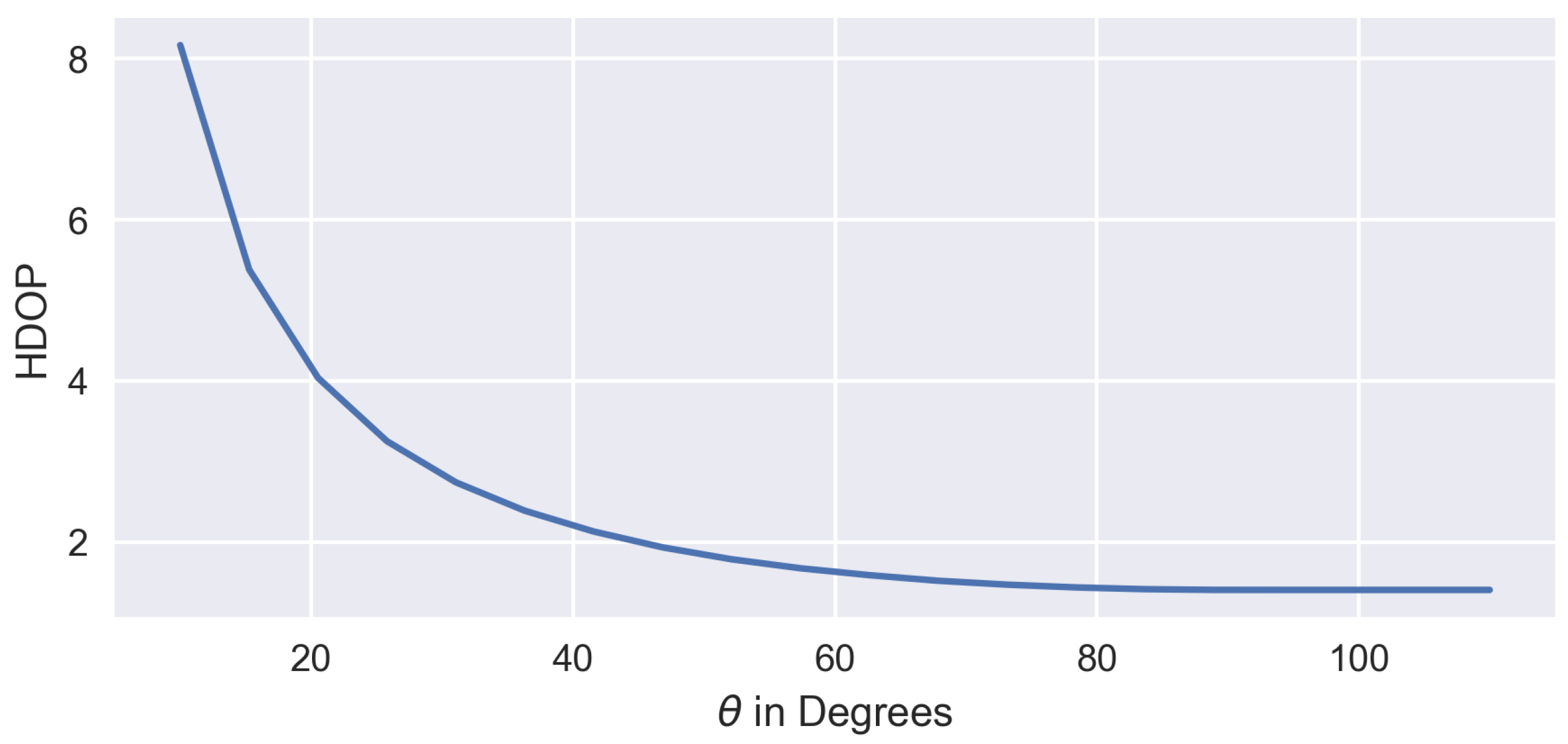
To optimize the geometry for multiple LF, an objective function must be derived that can be minimized using the optimization algorithm. An important property is the impact of a suboptimal geometry on the HDOP. For $M=2$ HF, HDOP is shown in Figure 4. Additionally, a threshold is set at $\mathrm{HDOP}=10$. During operation, the HF are affected from GNSS-based position estimation uncertainty and they may show unmodeled dynamics. For a position uncertainty of ${\sigma }_{r,GNSS}=2.5$ m and a safety factor of $s=3$, the feasible azimuth range is further reduced on both sides by

$${\Delta }_{\theta }={\tan }^{-1}\left(\frac{{\sigma }_{r,GNSS}·s}{R_{min}}\right)$$

(21)

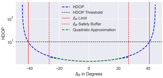
Figure 4. The effect of a suboptimal geometry for M = 2 HF on HDOP; threshold set at HDOP = 10, safety buffer with $R_{min}=20.0$, ${\sigma }_{r,GNSS}=2.5$ m, and $s=3$.

Here, $R_{min}$ is the minimum distance from the HF to an LF, which comes from the assumption that HF should have an elevation angle as low as possible to increase the observability of the LF position within the horizontal plane. Furthermore, it can be seen that within the safety buffer interval, the HDOP can be approximated using a quadratic function.

To visualize the effect of the safety buffer on the feasible area for HF positioning, the limits are shown in polar coordinates in Figure 5. It can be seen that rather than a direction, the feasible area is now a valid range in which the HDOP is likely to be below the value of $HDOP=10$.

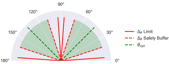
Figure 5. Valid azimuth ranges for $M=2$ HF; ${\Delta }_{\theta }$ limit found for $HDOP=10$; safety buffer includes position and maneuvering uncertainty.

3. Results

To illustrate the effectiveness of the feasible azimuth areas, an optimization example is given for $M=2$ HF and $N=3$ LF. For efficient computation, the problem is formulated using Cartesian coordinates. Instead of calculating the non-linear value of ${\Delta }_{\theta }$, the normal distance to the ${\theta }_{opt}$ vector is calculated, which underestimates the HDOP when close to the LF and overestimates it when further away. Note that the feasible azimuth areas are defined relative to each other. Here, both ${\theta }_{opt}$ lines are separated by ${90}^{\circ }$ from each other. By rotating the symmetry axis slightly in one direction, one could improve the HDOP as the ${\theta }_{opt}$ vectors might form a better joint geometry with those of other LF. Therefore, the optimization variables do not only consist of the HF positions, $q_i$, but also of the change in the symmetry axis–angle from ${90}^{\circ }$, ${\varphi }_j$. The orthogonal distance to the ${\theta }_{opt}$ vector is then given as

$$d_{n,ij}={(q_i-p_j)}^T(I+{\left[{\varphi }_i\right]}_x)w.$$

(22)

Here, $w\left({\theta }_{opt}\right)$ is the normal vector of the ${\theta }_{opt}$ vector and ${\left[{\varphi }_i\right]}_x$ the skew-symmetric matrix of $\varphi$. The objective function is then formed as a sum of squared errors (SSE), which is supported via the quadratic approximation of the HDOP error as a function of ${\Delta }_{\theta }$, as shown in Figure 4. Together with the minimum and maximum range constraints and the restriction of the feasible area to the valid azimuth areas, the optimization problem is defined as follows:

$$\begin{array}{cc}\hfill \underset{q_i,{\varphi }_i}{min}& \sum _{i=1}^M\sum _{j=1}^N{(q_i-p_j)}^T(I+{\left[{\varphi }_i\right]}_x)w\left({\theta }_{opt}\right)\hfill \\ \hfill \mathrm{s}.\mathrm{t}.& {(q_i-p_j)}^T(I+{\left[{\varphi }_i\right]}_x)w({\theta }_{opt}+{\Delta }_{\theta ,max})<0\hfill \\ \hfill & {(q_i-p_j)}^T(I+{\left[{\varphi }_i\right]}_x)w({\theta }_{opt}-{\Delta }_{\theta ,max})>0\hfill \\ \hfill & {(q_i-p_j)}^T(q_i-p_j)>R_{min}^2\hfill \\ \hfill & {(q_i-p_j)}^T(q_i-p_j)<R_{max}^2\hfill \\ \hfill & -{10}^{\circ }\le {\varphi }_i\le {10}^{\circ }\hfill \end{array}$$

(23)

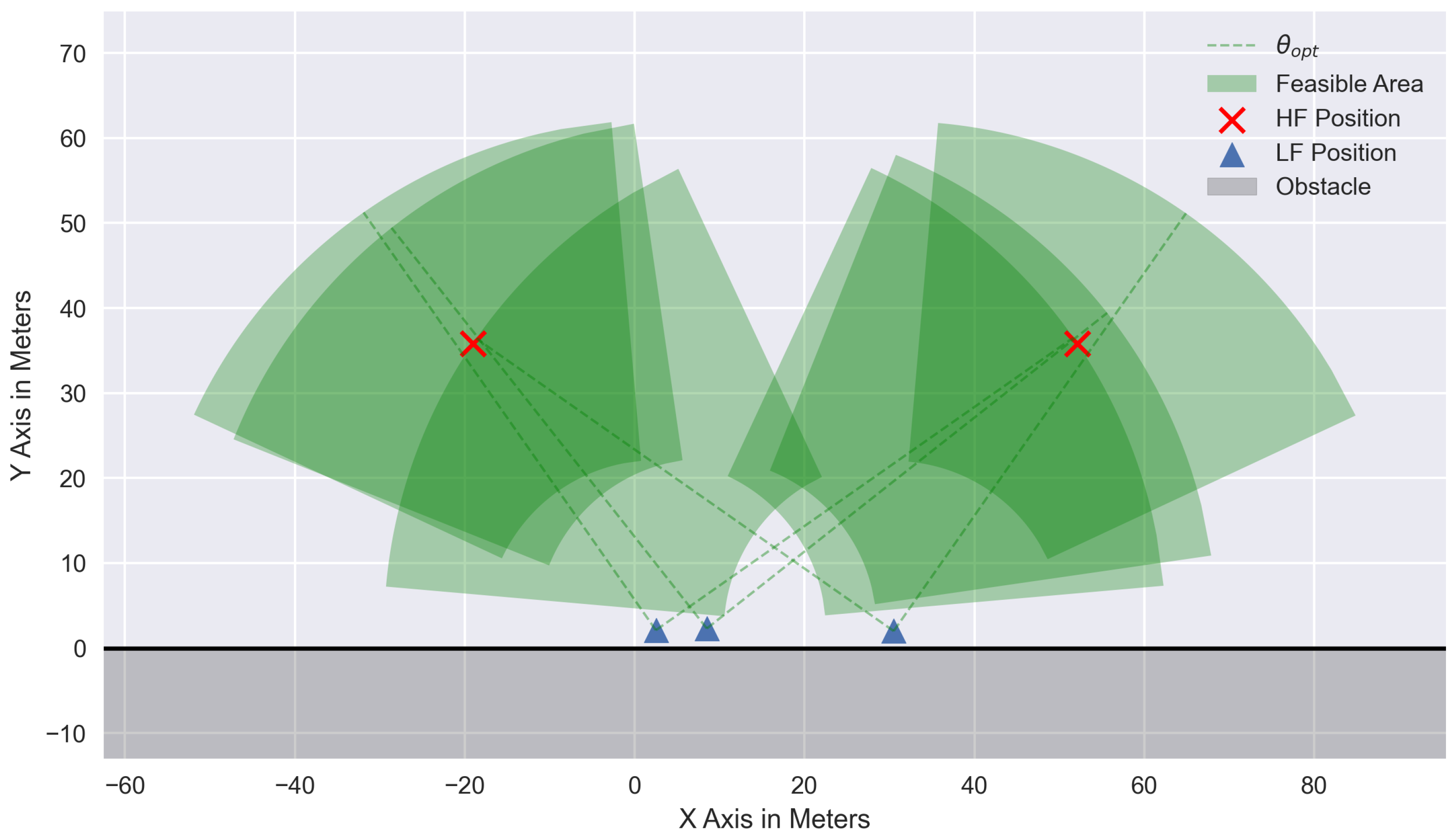
The optimization result is shown for one scenario in Figure 6. All LF operate close to an obstacle while two HF must be positioned such that the HDOP is optimized for all LF. The left two UAS tend to tilt their mirror axis towards the further distant LF on the right, while that UAS tilts the symmetry axis to the left such that the ${\theta }_{opt}$ vectors are nearly intersecting. Exactly at that point is when the optimization finds the optimal HF positions. For two HF, the minimum HDOP is $\sqrt{2}\sim 1.414$, while the found solution yields 0.039%, 0.054%, and 0.044% higher HDOP values for each of the LF.

Figure 6. Solution to the quadratic minimization problem of minimizing HDOP for all LF close to an obstacle; solution is constrained within the feasible azimuth areas; HDOP error $\sim 0.05\%$.

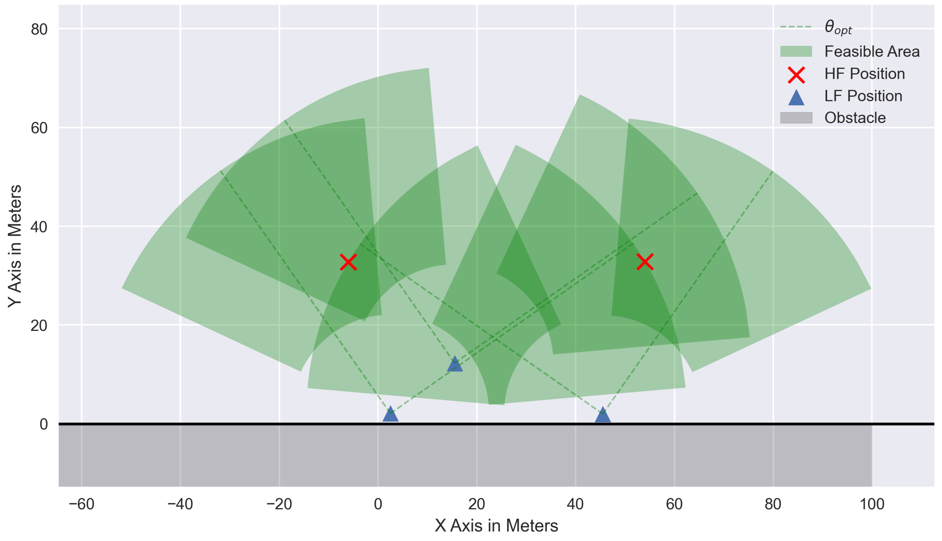
A less favorable scenario is shown in Figure 7. Here, the most outer LF are close to losing connectivity as they operate at $R_{max}$. Additionally, the middle LF is located at a further distance to the wall. This geometric deficiency of the LF configuration results in a worse HDOP, which is also reflected by the larger distance of the ${\theta }_{opt}$ vectors. Here, they are further from intersecting than in the first scenario. Compared to the minimum achievable HDOP, here they are 3.68%, 5.36%, and 3.72% higher.

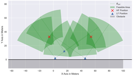
Figure 7. Solution to a less favorable scenario; sub-optimal geometry visible via intersection of all ${\theta }_{opt}$ vectors of one direction; HDOP error $\sim 5.4\%$.

For other configurations, a similar optimization could be applied. The presence of additional obstacles or non-convex obstacles can be incorporated by limiting the feasible $\theta$-range even further.

4. Conclusions

This paper provides insights into the optimal positioning of High-Flying UAS (HF) to aid the absolute horizontal navigation of Low-Flying UAS (LF) operating in GNSS-denied environments. The problem is formalized and is transformed into polar coordinates so it can be interpreted as an azimuth selection problem. For different numbers of HF, optimal azimuth angles are presented to minimize the Horizontal Dilution of Precision (HDOP) of an LF. As an example, an optimization problem is derived and solved for two HF aiding three LF. The resulting geometry has yielded promising HDOP values, guaranteeing an improved navigation performance in GNSS-denied environments. Future work will include online optimization for the multi-LF case as well as an extension to three-dimensional DOP. In conclusion, HF positioning constraints have been derived in a closed form which optimize the HDOP for one LF. For multiple LF, an algorithm is presented which improves the horizontal navigation performance of low-flying UAS in GNSS-denied environments.

References

- Braasch, M.S. Multipath. In Springer Handbook of Global Navigation Satellite Systems; Teunissen, P.J., Montenbruck, O., Eds.; Springer International Publishing: Cham, Switzerland, 2017; pp. 443–468. [Google Scholar] [CrossRef]
- de Haag, M.U.; Martens, M.; Huschbeck, S. Urban Swarm Navigation Exploiting sUAS Collaboration and Cognition. In Proceedings of the 2022 International Conference on Unmanned Aircraft Systems (ICUAS), Dubrovnik, Croatia, 21–24 June 2022; pp. 319–328. [Google Scholar] [CrossRef]
- Tiemann, J.; Schweikowski, F.; Wietfeld, C. Design of an UWB indoor-positioning system for UAV navigation in GNSS-denied environments. In Proceedings of the 2015 International Conference on Indoor Positioning and Indoor Navigation (IPIN), Banff, AB, Canada, 13–16 October 2015; pp. 1–7. [Google Scholar] [CrossRef]
- Yu, X.; Li, Q.; Queralta, J.P.; Heikkonen, J.; Westerlund, T. Cooperative UWB-Based Localization for Outdoors Positioning and Navigation of UAVs aided by Ground Robots. In Proceedings of the 2021 IEEE International Conference on Autonomous Systems (ICAS), Montreal, QC, Canada, 11–13 August 2021; pp. 1–5. [Google Scholar] [CrossRef]
- Kihara, M.; Okada, T. A Satellite Selection Method and Accuracy for the Global Positioning System. Navigation 1984, 31, 8–20. [Google Scholar] [CrossRef]
- Blanco-Delgado, N.; Nunes, F.D.; Seco-Granados, G. On the relation between GDOP and the volume described by the user-to-satellite unit vectors for GNSS positioning. GPS Solut. 2017, 21, 1139–1147. [Google Scholar] [CrossRef]
- Yang, B.; Yang, E.; Yu, L.; Loeliger, A. High-Precision UWB-Based Localisation for UAV in Extremely Confined Environments. IEEE Sens. J. 2022, 22, 1020–1029. [Google Scholar] [CrossRef]
Disclaimer/Publisher’s Note: The statements, opinions and data contained in all publications are solely those of the individual author(s) and contributor(s) and not of MDPI and/or the editor(s). MDPI and/or the editor(s) disclaim responsibility for any injury to people or property resulting from any ideas, methods, instructions or products referred to in the content. |
© 2023 by the authors. Licensee MDPI, Basel, Switzerland. This article is an open access article distributed under the terms and conditions of the Creative Commons Attribution (CC BY) license (https://creativecommons.org/licenses/by/4.0/).