Abstract
Unsteady airfoils play a pivotal role in comprehending diverse aerospace applications, being one of those flapping propulsions. The present paper studies this topic by bringing back an old unsteady panel method to juxtapose its results against CFD data previously obtained. The central objective is to revive the interest in these reduced order models in the topic of unsteady airfoils, which can be extended to model highly nonlinear effects while keeping computational resources fairly low. The findings reveal that while the potential flow-based UPM (Unsteady Panel Method) struggles to accurately capture the airfoil’s propulsive power, it remains adept at estimating consumed power. Moreover, an investigation into the pressure coefficient shows the potential benefits of UPM in contexts where flow separation can be disregarded. Despite inherent limitations, these simplified methodologies offer an effective preliminary estimation of flapping airfoil propulsive capabilities.
1. Introduction
Studying flapping airfoils provides a much-needed understanding regarding several challenges and technologies, for instance, natural and unconventional flight and the dynamics of micro and nano air vehicles.
When looking at the lower spectrum of the Reynolds number, flapping airfoils becomes an attractive solution regarding propulsion. Early work [1,2] has suggested that an unsteady airfoil creates an effective angle of attack which could lead to the resultant force being decomposed into lift and thrust. This was later updated by looking at the airfoil’s wake [3], which, based on the vortices rotation and position, would denounce if the airfoil was in a drag or thrust regime.
Years later, the problem was first addressed analytically by Theodorsen [4] who predicted unsteady aerodynamics of pitching and plunging airfoils, although with some clear limitations. A year later, Garrick [5] extended Theodorsen’s formulation study of an airfoil or an airfoil–aileron configuration flapping with three degrees of freedom. The problem was then studied numerically by employing an unsteady panel code [6] and its results were compared with experimental data. Its results showed that the panel code could predict the formulation and evolution of the thrust wake structures, and concluded that these are governed by essentially inviscid phenomena. While these models can provide a good prediction of the aerodynamic behavior of unsteady airfoils, they present severe weaknesses regarding flow separation at the leading edge which the airfoil experiences at higher angles of attack [7]. Nevertheless, it can still provide an approximate estimate of the trailing-edge vortex formation and its convention, which is an overall inviscid phenomenon.
Combining these limitations with the emergence of CFD and the availability of computational power, these methods have become out of use. However, these simpler techniques and reduced-order models can still provide an efficient way to obtain an overall comprehension of the problem. Furthermore, these could be enhanced by modeling highly nonlinear effects such as dynamic stall. Hence, this work has the objective of reviving interest in unsteady panel methods (UPMs) and comparing its results with CFD computations at low Reynolds numbers where the profound dynamic stall is present.
2. Methodology
The present study focuses on the propulsive capabilities of flapping airfoils estimated via a panel method using potential flow, in particular, the performance of the NACA0012-IK30 airfoil proposed by us [8]. The results are contrasted against high-fidelity CFD simulations conducted using Ansys© Fluent 2022 R1. These simulations used a RANS (Reynolds-Averaged Navier–Stokes) approach, referring to the SST turbulence model coupled with the intermittency transition model. For further details, regarding other numerical methods, model validation, and specific CFD results which will be used here, we refer you to our previous work [9].
The current methodology that governs the panel method is based on the extension of the Hess-Smith Panel Method (HSPM) to unsteady flows used by Teng [10]. The extension of the Hess-Smith Panel Method, as in the steady case formulation, assumes that the airfoil surface is discretized into several panels and is represented by singularity distributions of source strength at each panel () and a vorticity over the airfoil surface, varying both in time. Hence, the subscript k is used to indicate the current time-step (), at which the singularity distribution of the source strength is and vorticity is .
In unsteady flows, according to Helmholtz and Kelvin’s circulation theorems, the total circulation in the flowfield must remain constant. This means that when there is a change in circulation on the airfoil surface, there must be an equal and opposite change in the wake vorticity, which can be obtained as a vortex-shedding process at the trailing edge of the airfoil.
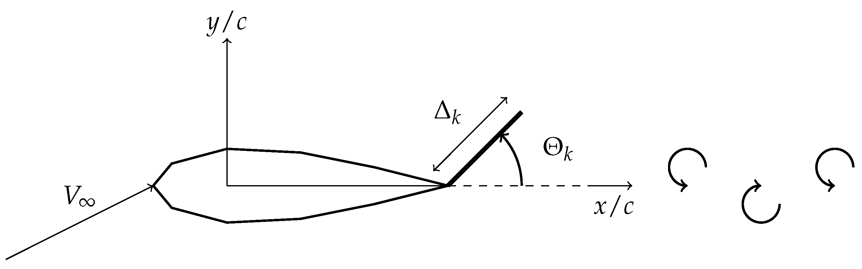
So, at each time step, to model such a vortex shedding process, an additional panel with length and inclination to the x-axis is attached to the trailing edge with a uniform vorticity distribution , as shown in Figure 1.
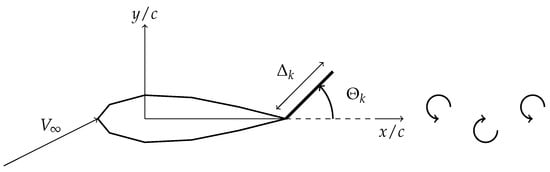
Figure 1.
Unsteady potential flow formulation (airfoil-fixed frame).
With this extra panel at the trailing edge, to verify the Helmholtz and Kelvin theorems, Equation (1) should be applied.
which may be written as
where ℓ is the airfoil perimeter.
Regarding the length and orientation of the extra panel, the assumptions of Basu and Hancock [11] are used. These hypotheses make the following statements:
- The additional vorticity panel has the direction of the local resultant velocity at the panel midpoint.
- The length of the additional panel depends on the results’ velocity at the panel midpoint and the size of the timestep.
After finding the trailing edge panel characteristics, it is shed to the wake and convected as a concentrated free vortex by the flowfield with circulation .
In addition to the conservation of the flow field circulation, one should also impose the boundary condition where there is no permeability at the wall. Thus,
Moreover, there is the need to impose the Kutta condition, but, unlike the steady case, the rate of change of potential at the trailing edge should now be included, which is linked to the total circulation rate of change.
where a backward finite difference is used to approximate the rate of change of total circulation as
The numerical solution of this panel method is composed of three main stages. The first concerns the calculation of influence coefficients which hold information on how each fluid element influences all others, with some being time-dependent. The second phase passes by employing the flow tangency solution and forcing the Kutta condition iteratively. The third and last step regard the determination of the pressure distribution and force calculations. For the specifics of the mathematical formulation, we refer you to the work of Teng [10].
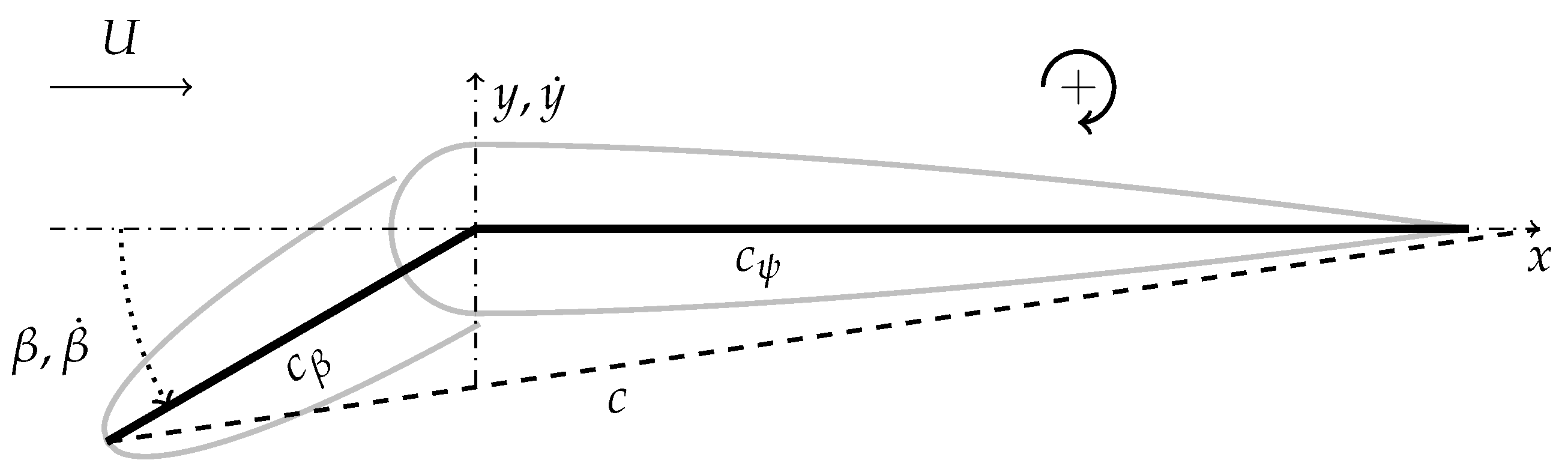
As mentioned before, the central element in the study is the NACA0012-IK30 airfoil. As illustrated in Figure 2, this airfoil is a modification of the conventional NACA0012, where it has been segmented into two parts ( and ) with a pivot at 30% of the chord.
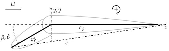
Figure 2.
Scheme of NACA0012-IK30 airfoil.
For the present study, the airfoil kinematics are governed by
where A, , and f are the plunging amplitude, leading-edge pitching amplitude, and frequency, respectively. Based on kinematics and geometric parameters, the angle of attack and effective angle of attack are calculated as
where U is the freestream velocity.
To analyze the propulsive performance, two coefficients were used: the propulsive power and mean required power coefficients. The first is defined as
which has the same value as the thrust coefficient. All force coefficients are obtained by integrating the pressure coefficient in the desired directions. The pressure coefficient is calculated by
where is the unsteady stream velocity that is observed on a coordinate system fixed on the airfoil, and V is the total velocity with respect to the airfoil-fixed coordinate system.
Regarding the required power coefficient, it is given by
where is the pitching moment of the part calculated at the pivot. The term is not considered as no pitching is prescribed to the back part.
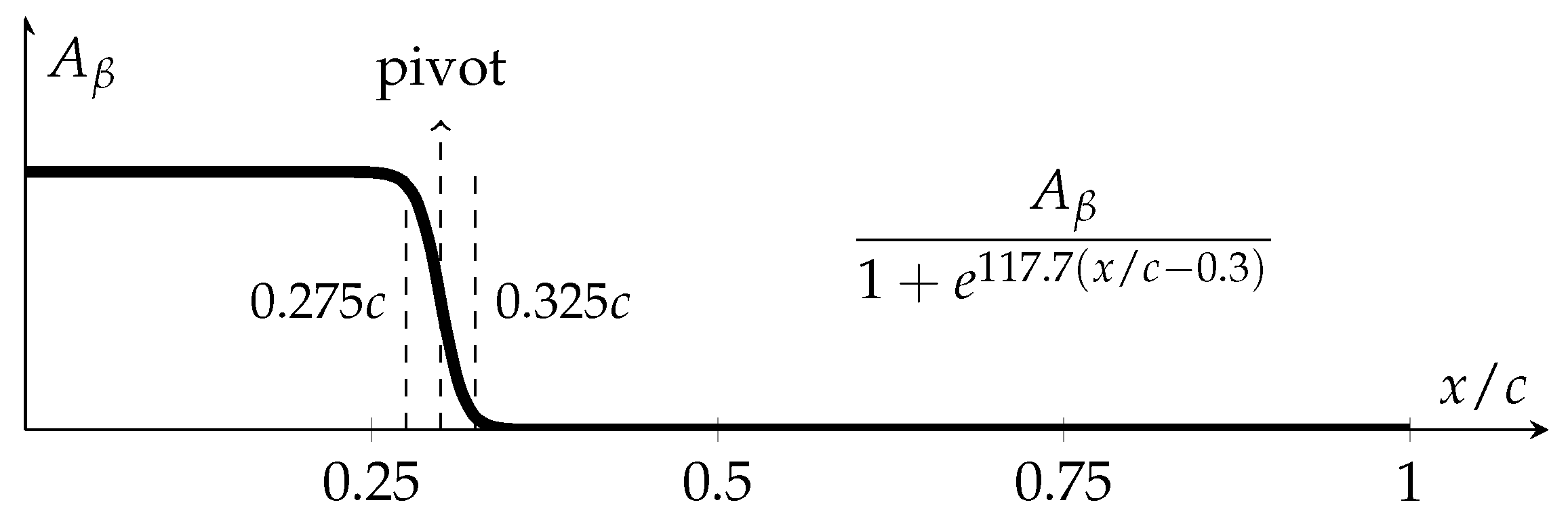
As observed, the proposed geometry has two discontinuities on the airfoil surface, presenting a clear challenge of the panel method. Without any consideration, if we deflect the frontal part, some control points (points separating panels) may overlap or grossly misrepresent our geometry. To tackle this challenge, we use an optimized sigmoid which provides a smooth transition using 5% of the airfoil chord to create a continuous deformation, as seen in Figure 3.
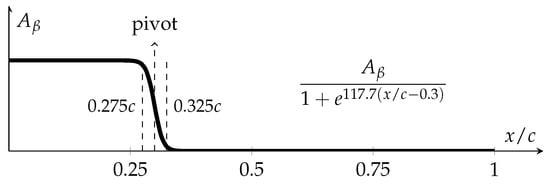
Figure 3.
Deformation strategy for the leading-edge deflection.
3. Results and Discussion
In this section, we present a comparison between previously published data obtained with CFD computations [9] against the ones obtained by the unsteady panel code. These computations are carried out at a Reynolds number of , two nondimensional amplitudes (h), and , and two nondimensional velocities (), and . For each of these conditions, the leading edge is deflected with three pitching amplitudes, 0, 10, and 20, closely following Equation (8).
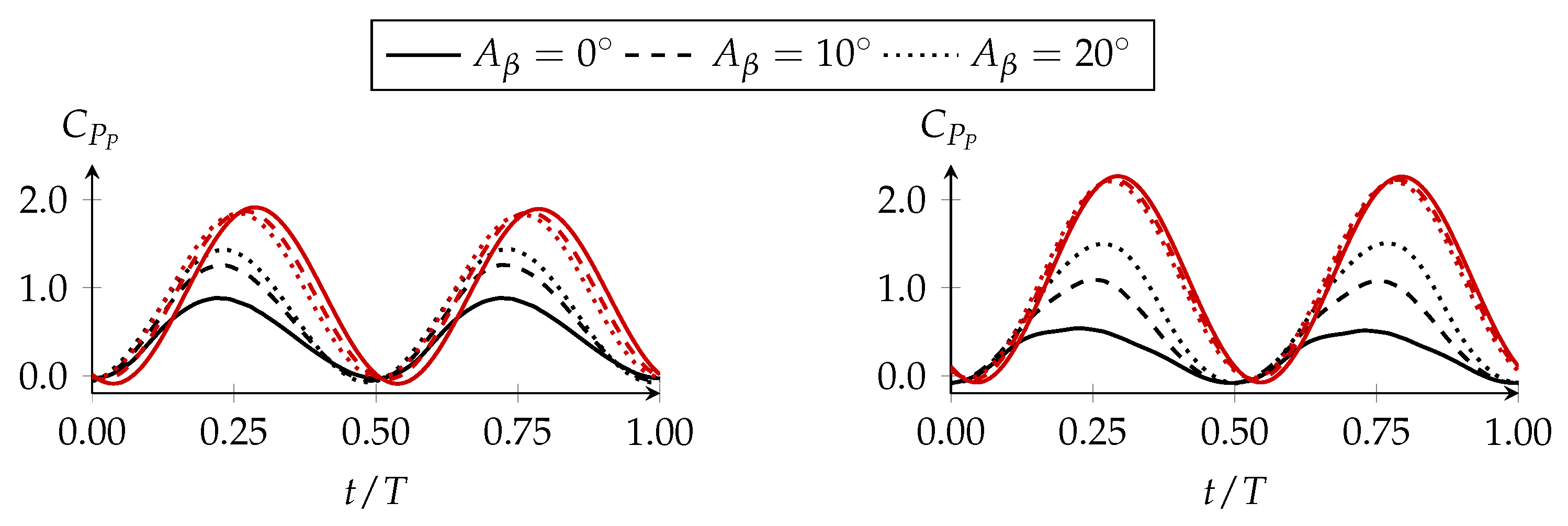
Starting with Figure 4, where the condition is shown for the two amplitudes, we first observe that in the CFD results, deflecting the leading edge up to 10 provides an increase in thrust produced, regardless of h. This has been linked to exploiting the presence of the suction zone in the larger frontal area of the airfoil created by [9]. When looking at the UPM results, it is clear that there is an overestimation of the thrust production, mainly due to the lack of separated flow, as seen ahead. Furthermore, deflecting the leading edge will lead to a slight thrust reduction which is caused by the lowering of the suction zone located at the frontal part of the airfoil, also shown afterwards.
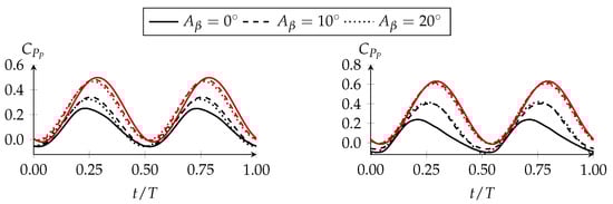
Figure 4.
as a function of with for (left) and (right). CFD and UPM results in black and red, respectively.
With a larger nondimensional velocity of , as shown in Figure 5, the airfoil is under extreme plunging. In fact, at this plunging velocity, its effective angle of attack reaches 45, which undeniably leads to the formation of extensive regions of separated flow. The graphs present the same conclusions as before, with real flow being favored by the leading-edge deflection, while the inviscid solution is not. However, it is interesting to see how deflecting the leading edge pushes the CFD results closer to the inviscid solution. This may be because deflecting the leading edge in real flow can lead to the minimization of the flow separation, which is a regime where potential flow truly stands out. Additionally, it is worth mentioning that during the accelerating phases, 0.00–0.25 and 0.50–0.75, the panel method provides a good approximation, which may denounce that this is a time window where none or negligible separation is present.

Figure 5.
as a function of with for (left) and (right). CFD and UPM results in black and red, respectively.
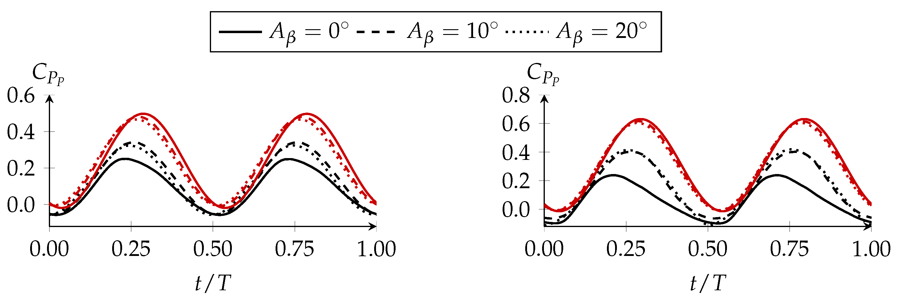
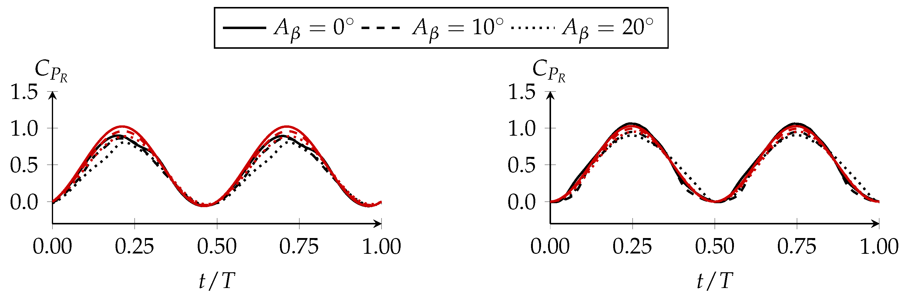
Moving to Figure 6, we now present the required power coefficient for and both amplitudes. Contrarily to the propulsive power, the panel code provides a very good prediction of the consumed power for the two amplitudes. Additionally, as in the CFD computations, deflecting the leading edge provides a slight reduction in the consumed power due to lowering the effective angle of attack.
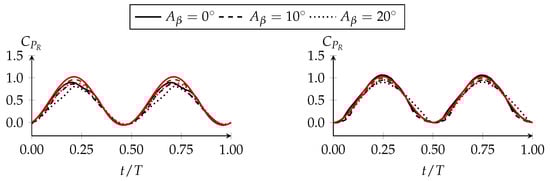
Figure 6.
as a function of with for (left) and (right). CFD and UPM results in black and red, respectively.
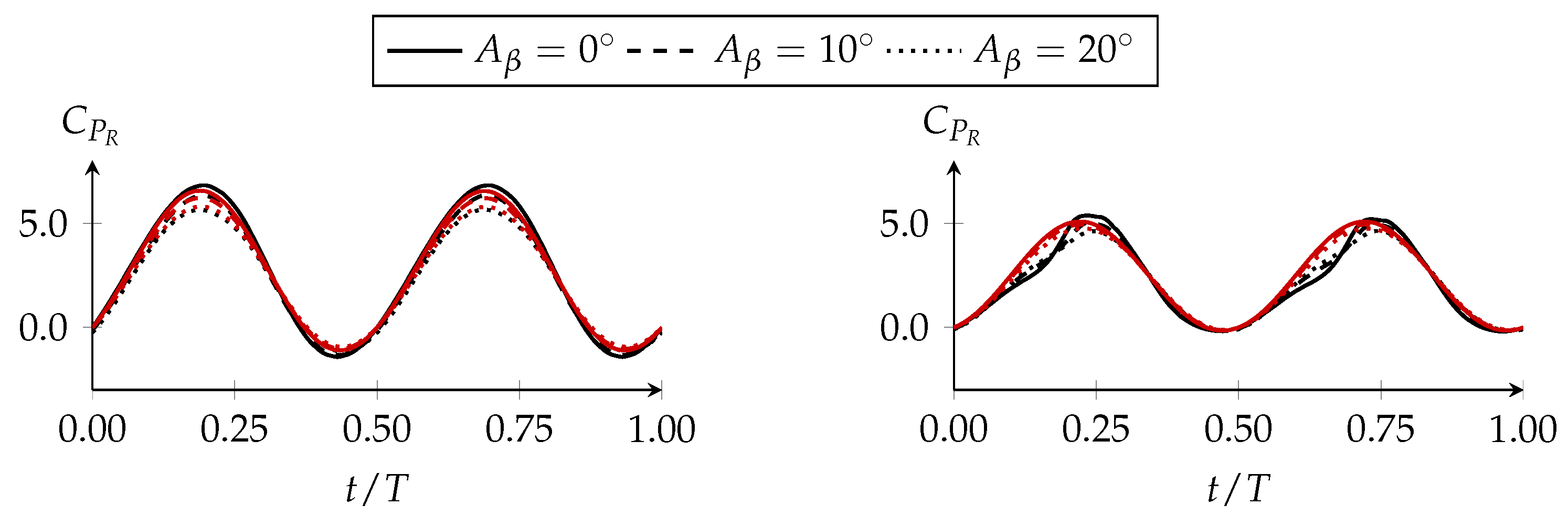
With , as illustrated in Figure 7, the panel code can still provide an adequate approximation. This is a very interesting result since this is a condition where severe flow separation is present, and still the potential flow approach can predict the lifting forces quite accurately, and thus the consumed power.
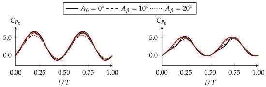
Figure 7.
as a function of with for (left) and (right). CFD and UPM results in black and red, respectively.
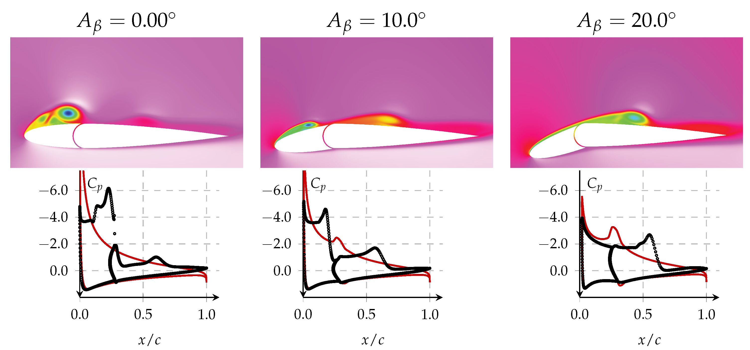
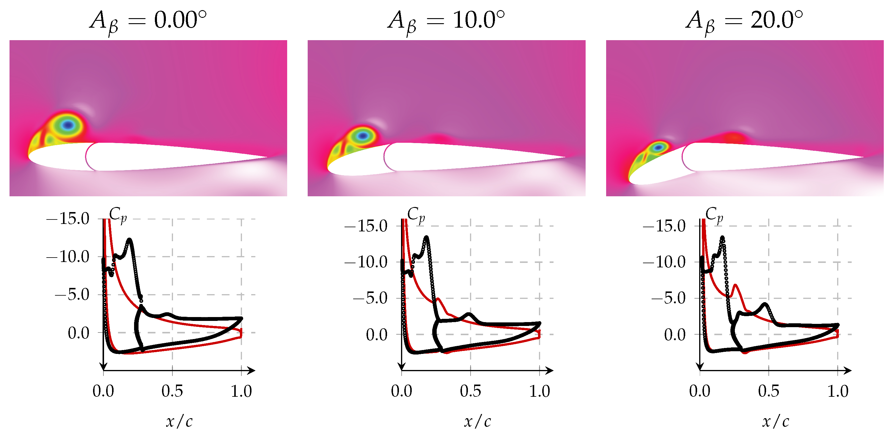
To better grasp the propulsive coefficients presented before, Figure 8 shows the pressure contours obtained using CFD and the pressure coefficients of both CFD and UPM simulations. All data correspond only to the larger amplitude () and at , which is when the airfoil is halfway down, presenting its maximum plunging velocity and leading edge deflection.
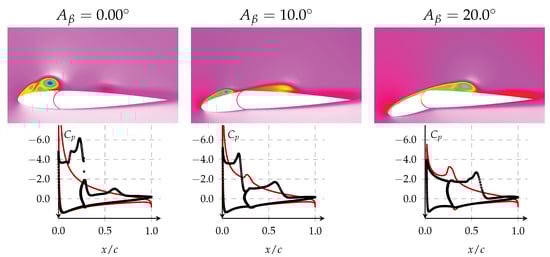
Figure 8.
CFD pressure contour and pressure coefficient for and at . CFD and UPM results in black and red, respectively.
As expected, the panel method presents an extremely high suction peak at the leading edge, which cannot be sustained in real flow. This is confirmed by the presence of a leading-edge vortex in the CFD results. Additionally, it is also seen that a low-pressure zone is present at the back part, where CFD shows a bump in the pressure coefficient. Interestingly enough, the panel code also has this prominence, although for a much different reason. Due to the leading-edge deflection, the whole airfoil presents what may be considered a dynamic curvature, being maximum at the pivot point (). With this curvature, a low-pressure zone is needed around the pivot to guarantee that the air remains attached to the surface. This is the reason why the UPM presents this bump and not because of highly nonlinear effects such as vortex shedding. It is also worth mentioning that as the leading-edge pitching amplitude increases, the UPM starts offering a better aerodynamic representation of the pressure distribution, especially at the frontal part. This may be attributed to the absence of extreme flow separation.
Similar effects are seen in Figure 9, where the nondimensional velocity has been increased to . The results show the same limitations that arise from a potential flow approach, but some regions of the airfoil, for instance, the lower surface, are well represented by the UPM solution.
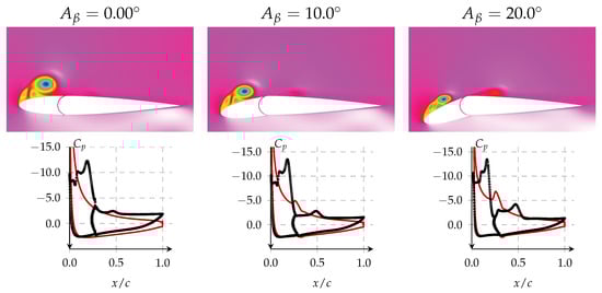
Figure 9.
CFD pressure contour and pressure coefficient for and at . CFD and UPM results in black and red, respectively.
4. Conclusions
Unsteady airfoils are studied as a means to understand several aerospace applications. At lower velocity and length scales, their propulsive potential becomes undeniable. However, studying numerically using CFD is quite complex, typically requiring a higher level of computing power, which makes reduced-order models very attractive.
The present paper reintroduced an unsteady panel method and its results were compared with pressure fields obtained in CFD simulations. The results indicated that the propulsive power of the airfoil cannot be accurately modeled with potential flow due to the limitless suction peak created by the UPM. However, when it comes to the consumed power, the panel method provides a good first estimate. The pressure coefficient was also analyzed at two different cycle stages, where we saw that the UPM approach could be beneficial in conditions where flow separation could be neglected.
Although with several limitations, these simpler methods provide an efficient way to obtain a first estimate of the propulsive capabilities of flapping airfoils. Future work will be focused on extending the UPM by modeling some level of vortex shedding mechanism which could improve the estimation of thrust generation.
Author Contributions
Conceptualization, E.A.R.C.; methodology, E.A.R.C. and A.R.R.S.; validation, E.A.R.C.; formal analysis, E.A.R.C., A.R.R.S., and F.D.M.; investigation, E.A.R.C.; data curation, E.A.R.C.; writing—original draft preparation, E.A.R.C.; writing—review and editing, A.R.R.S. and F.D.M.; supervision, A.R.R.S. and F.D.M.; project administration, A.R.R.S. and F.D.M.; funding acquisition, A.R.R.S. and F.D.M. All authors have read and agreed to the published version of the manuscript.
Funding
This research was funded by Portuguese’s Fundação para a Ciência e Tecnologia (FCT) under grant numbers UIDB/50022/2020, UIDP/50022/2020, LA/P/0079/2020, 2020.04648.BD, and by Brazil’s National Council for Scientific and Technological Development (CNPq grant #306824/2019-1).
Institutional Review Board Statement
Not applicable.
Informed Consent Statement
Not applicable.
Data Availability Statement
The data presented in this study are available on request from the corresponding author. The data are not publicly available due to privacy.
Conflicts of Interest
The authors declare no conflicts of interest.
References
- Betz, A. Ein beitrag zur erklaerung segelfluges. Z. Flugtech. Mot. 1912, 3, 269–272. [Google Scholar]
- Knoller, R. Die gesetzedes luftwiderstandes. Flug-Und Mot. 1909, 3, 1–7. [Google Scholar]
- Kármán, T.; Burgers, J.M. General Aerodynamic Theory: Perfect Fluids; Springer: Berlin/Heidelberg, Germany, 1935. [Google Scholar]
- Theodorsen, T. General Theory of Aerodynamic Instability and the Mechanism of Flutter; NACA Technical Report; NACA: Washington, DC, USA, 1935. [Google Scholar]
- Garrick, I.E. Propulsion of a flapping and oscillating airfoil. In Report National Advisory Committee for Aeronautics, NACA Report 567; NACA: Washington, DC, USA, 1936; pp. 419–427. [Google Scholar]
- Jones, K.D.; Dohring, C.M.; Platzer, M.F. Experimental and Computational Investigation of the Knoller-Betz Effect. AIAA J. 1998, 36, 1240–1246. [Google Scholar] [CrossRef]
- Platzer, M.F.; Jones, K.D.; Young, J.; Lai, J.C.S. Flapping Wing Aerodynamics: Progress and Challenges. AIAA J. 2008, 46, 2136–2149. [Google Scholar] [CrossRef]
- Camacho, E.A.; Neves, F.M.; Marques, F.D.; Barata, J.M.; Silva, A.R. Effects of a Dynamic Leading Edge on a Plunging Airfoil. In Proceedings of the AIAA Aviation 2021 Forum, Online, 2–6 August 2021. [Google Scholar] [CrossRef]
- Camacho, E.A.R.; Marques, F.D.; Silva, A.R.R. Influence of a Deflectable Leading-Edge on a Flapping Airfoil. Aerospace 2023, 10, 615. [Google Scholar] [CrossRef]
- Teng, N.H. The Development of a Computer Code (U2DIIF) for the Numerical Solution of Unsteady, Inviscid and Incompressible Flow Over an Airfoil; Technical Report; Naval Postgraduate School: Monterey, CA, USA, 1987. [Google Scholar]
- Basu, B.C.; Hancock, G.J. The unsteady motion of a two-dimensional aerofoil in incompressible inviscid flow. J. Fluid Mech. 1978, 87, 159–178. [Google Scholar] [CrossRef]
Disclaimer/Publisher’s Note: The statements, opinions and data contained in all publications are solely those of the individual author(s) and contributor(s) and not of MDPI and/or the editor(s). MDPI and/or the editor(s) disclaim responsibility for any injury to people or property resulting from any ideas, methods, instructions or products referred to in the content. |
© 2023 by the authors. Licensee MDPI, Basel, Switzerland. This article is an open access article distributed under the terms and conditions of the Creative Commons Attribution (CC BY) license (https://creativecommons.org/licenses/by/4.0/).