Abstract
Crime forecasting has gained popularity in recent years; however, the majority of studies have been conducted in the United States, which may result in a bias towards areas with a substantial population. In this study, we generated different models capable of forecasting the number of crimes in 83 regions of Costa Rica. These models include the spatial–temporal correlation between regions. The findings indicate that the architecture based on an LSTM encoder–decoder achieved superior performance. The best model achieved the best performance in regions where crimes occurred more frequently; however, in more secure regions, the performance decayed.
1. Introduction
Police departments can use crime forecasting to plan where and when to carry out operations. There are countries that generated forecasting models to predict when crimes will happen and use predictive policing [1]. This action improves the efficiency in the distribution of police forces. According to [2], there is empirical research that has shown how strategies derived from crime prediction led to its reduction. Additionally, the forecasting of the number of crimes can be useful to evaluate the effectiveness of the strategies employed to combat the crime, comparing the prediction with the real cases. Predictions can be used as a measurement of the contrafactual of a police strategy. In areas like marketing, the forecasting of sales is used to set and monitor performance goals, and in the same way, the forecasting of crimes can be used by police forces.
Although crime prediction has gained popularity recently, most studies have been developed in the United States and are biased toward areas with a high population [3]. Therefore, it is convenient to analyze the performance of models for different areas. For simplicity, a model should be able to predict the crime number of multiple regions of a country or area of interest. The objective of this investigation is to conduct a comparison between the performance of various deep learning architectures in predicting crime across multiple regions for a small nation such as Costa Rica. Specifically, our models can be used to predict the crimes in any of the 83 regions that the country is divided into. These regions are called cantones.
Deep learning models have shown good performance in several time series tasks [4,5,6]; however, they have received little attention in crime forecasting; therefore, our study contributes to analyzing the performance of deep learning models in crime prediction.
According to [7], it is relevant that crime forecasting models consider the spatial–temporal correlations between regions because the occurrence of crimes in a region could influence the occurrence of crimes in other regions. However, this is often ignored in most models [7]. In our deep learning models, we consider the spatial–temporal correlations between regions, including the lags of the five regions that are more correlated with the count of crimes in each region. To identify these five regions, we followed a procedure based on partial autocorrelations.
In summary, the novel contributions of this manuscript are as follows:
- ✓
- Comparisons between deep learning models that are capable of forecasting crimes for multiple regions.
- ✓
- The incorporation of the spatial–temporal correlations between regions in the models and evaluation of its influence on the prediction performance.
- ✓
- The evaluation of the performance of models for crime prediction in a small country.
2. Literature Review
Crime forecasting research requires the definition of the temporal and spatial units of inference. In the literary review of [3], it is found that the most common temporal granularity of prediction is monthly, although studies are using annual, weekly, daily, and hourly ranges. The inference space is also diverse; several studies divide the main region of analysis into uniform areas of the same sizes, ranging from 75 m × 75 m onwards [3]. Other studies do not make uniform divisions but rather focus on specific regions [8,9].
Recent research has shown positive results with deep learning models. For example, in [10], the authors compare the performance of a stacked LSTM-based model with Auto ARIMA models to forecast the number of times 13 different types of crimes will occur in the next 12 months. In crimes such as bicycle theft, burglary, weapon possession, public order, robbery, vehicle crime, and total crime, the best-performing model comes from a deep learning model, while in others, the best result comes from Auto ARIMA. In [11], the authors compare LSTM with a direct H-step strategy in relation to SARIMA, for the monthly crime prediction of the Chicago Dataset. According to the results, the LSTM model had better performance. The authors of ref. [7] propose a Seq2Seq-based encoder–decoder LSTM model to predict the subsequent week of total daily crime in Brisbane and Chicago cities. The study reveals that the proposed model can capture and learn long-term dependencies from time series. In [9], the authors improved the ST-3DNet model to make it suitable for the crime prediction domain. The results showed that this model reduces the RMSE in relation to other models like SVR and LSTM for hourly crime prediction.
In [1], a novel hybrid method of Bi-LSTM and Exponential smoothing to predict the number of crimes per hour in New York was developed. The proposed approach outperformed as compared to state-of-the-art Seasonal Autoregressive Integrated Moving Averages (SARIMA) with a low mean absolute percentage error (MAPE).
Stec and Klabjan [12] combine convolutional neural networks with recurrent networks to predict the total number of crimes that will occur daily in the cities of Chicago and Portland. In the same line, ref. [13] created three architectures of deep learning based on the combination of neural networks to identify hot spots. The combination of the CNN + LSTM gave the best results.
Recent developed models use self-attention for daily forecasts. For example, ref. [14] developed a model to capture the dynamic spatio-temporal dependencies while keeping the model’s architecture reasonably interpretable. The authors of ref. [15] proposed an encoder–decoder architecture that possesses adaptive robustness for reducing the effect of outliers and waves in the time series.
Machine learning models do not always obtain the best performance in crime forecasting. For example, ref. [16] found the best results in classical models like ARIMA when the seasonal component was extracted from the time series. In order to compare the performance of deep learning models with a classical statistical model, we implemented SARIMAX. We chose SARIMAX instead of SARIMA to include multiple variables in the prediction of a time series as we conducted in the deep learning models.
3. Materials and Methods
3.1. Data
We used the property crime records that occurred in Costa Rica from 1 January 2015 to 30 May 2023. The records were collected by the Costa Rican Judicial Research Department (OIJ). The dataset contains information about the region and time when the crime report occurred. We aggregated the information per week (441 weeks) and month (101 months) in order to work with this periodicity.
Costa Rica is divided into 7 areas named provincias and 83 sub-areas named cantones. There are local governments for each canton; therefore, we decided to use the canton as the spatial unit of analysis in this study. The raw datasets are in the following: https://github.com/martin12cr/crimeCR (accessed on 25 September 2023).
3.2. Models
We generated five models of deep learning and SARIMAX models for the monthly and weekly datasets. These are as follows:
- SARIMAX models were developed using the auto.arima function of the pmdarima Python module. AIC criteria in 25 iterations were applied to select the configuration of the best model.
- Long short-term memory (LSTM) with three layers: input layer + LSTM (for month and week (recurrent units = 60, activation = linear)) + dense layer. The learning rate was 0.0001 for month and week.
- Temporal Convolutional Network (TCN) with three layers: input layer + TCN (for month (132 filters, kernel = 2, activation = tanh), for week (12 filters, kernel = 6, activation = linear)) + dense layer. The learning rate was 0.0001 for month and 0.01 for week.
- Encoder transformer with the following: input layer+ multi-head attention (for month (head size = 512, heads = 2), for week (head size = 128, heads = 4)) + dropout (for month 30% and for week 20%) + layer normalization+ convolutional 1D + dropout (for month 30% and for week 20%) + convolutional 1D + layer normalization + multi-head attention (for month (head size = 512, heads = 2), for week (head size = 128, heads = 4)) + dropout (for month 30% and for week 20%) + layer normalization + convolutional 1D + dropout (for month 30% and for week 20%) + convolutional 1D + layer normalization + global average pooling 1D + dense layer (256, activation = linear) + dropout (for month 30% and for week 20%) + dense layer (128, activation = linear) + dropout (for month 30% and for week 20%) + dense layer. The learning rate was 0.0001 for month and 0.001 for week.
- Classical transformer encoder–decoder with the following: input layer + two encoders (head size = 512, heads = 8, feed forward encoder = 2048, dropout = 20%) + two decoders (head size = 512, heads = 8, feed forward decoder = 2048 + dropout = 20%).
- LSTM encoder–decoder with the following: input layer + encoder LSTM (for month (60 recurrent units, activation = linear), for week (108 recurrent units, activation = tanh)) + decoder LSTM (for month (60 recurrent units, activation = linear), for week (108 recurrent units, activation = tanh)) + time distributed layer (output Is obtained separately for each time step). The learning rate was 0.001 for month and 0.0001 for week.
The hyperparameters of models were defined in the training phase through Bayesian optimization. We used early stopping to determine the number of epochs, and the loss function was the mean absolute error.
3.3. The Input–Output of the Models
For the monthly models, the inputs were the information about the 12-month lags of the next variables: the count of crimes of region j, the count of crimes of the five regions that are more correlated with region j, the month of the year, and the code of the region for the 12-month lags.
The outputs were the next 12 months. In the case of the weekly models, we used the same variables, but the input was the past 8 weeks and the output the next 8 weeks. Table 1 shows an example of the input array and output vector for one weekly instance. We concatenated the instances of all regions in order to create a model that can predict for any region.

Table 1.
An example of an instance for the input and output of the weekly model.
3.4. Spatial–Temporal Correlation
For the identification of the regions more related to the count of crimes of a region j, we applied the next procedure:
- Compute the partial autocorrelations between the time series and the 8 lags (12 lags for the monthly dataset) of the remaining time series.
- Obtain the average partial autocorrelations between the time series and the remaining time series.
- Obtain the top 5 average partial autocorrelations to identify the regions more related to the count of crimes of region j.
3.5. Experimental Procedure
We used cross-validation on a rolling basis to evaluate the models’ performance and make comparisons between them. Three partitions in the training and test were generated. Two metrics were used to compare the performance of the models: the mean absolute error (MAE) and a modified version of the MAPE. The modification was to add one unit to the vector of real values and to the vector of predictions, to avoid the no-definition when there were no crimes in a specific spatial–temporal range. In the dataset, it is common to find records where no crimes occurred. This situation generates no-definition when the classical MAPE is computed. The formula is the following:
where = real value, = prediction, n = forecast horizon.
4. Results
Although the models were generated to predict a horizon of 12 months and 8 weeks, we also analyzed the performance of 3 months and 2 weeks, using only the first values of the prediction vector. Additionally, for each model, we obtained the performance metrics for the 82 regions and the three test partitions.
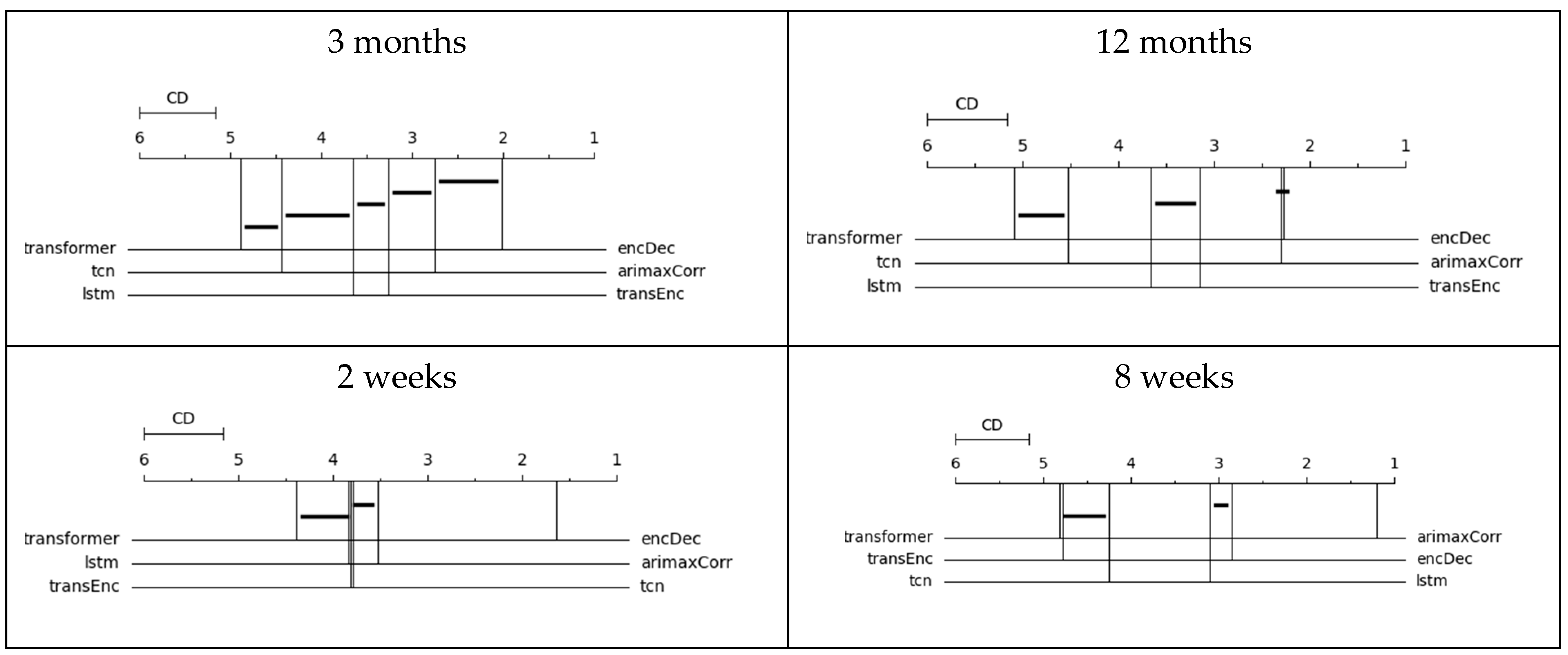
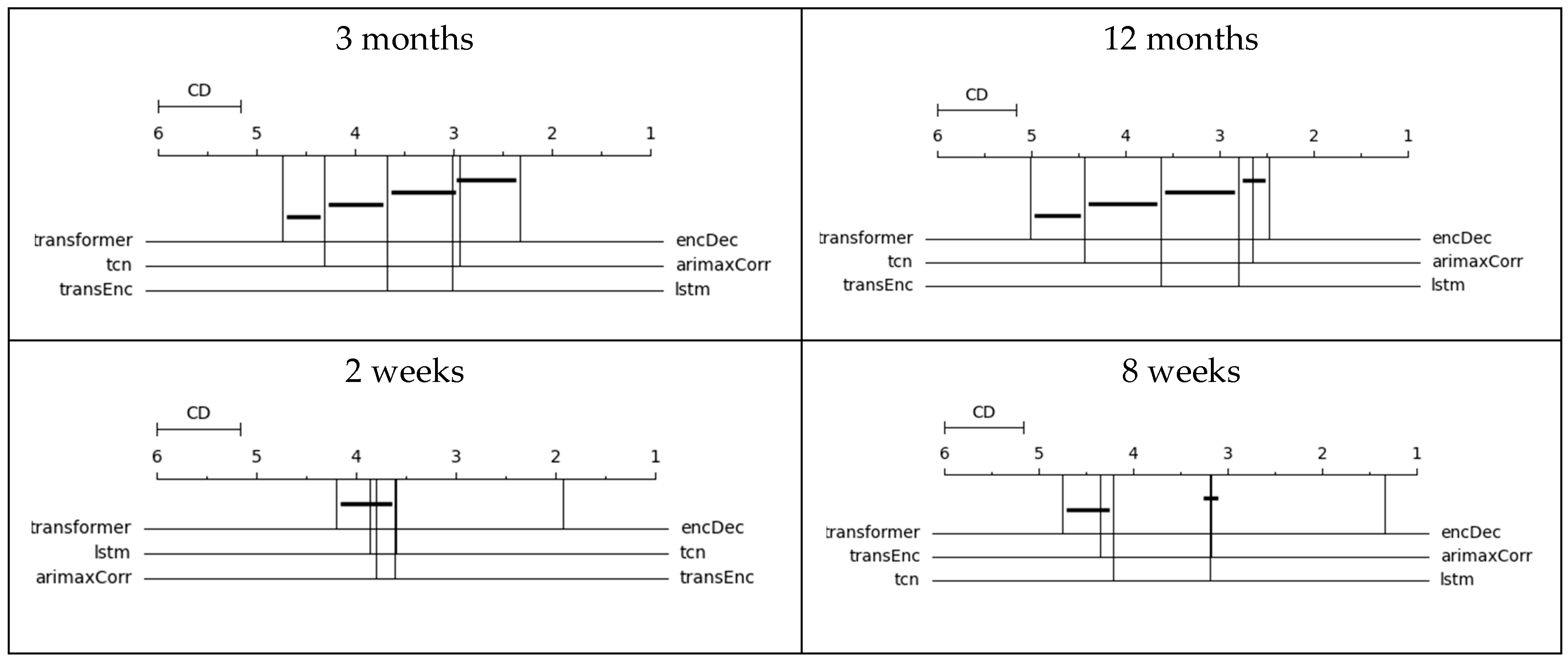
To determine if there are significant statistical differences between models, CD diagrams were generated, following the procedure of the package autorank from Python [17]. The CD diagrams show the average rank of each model. The horizontal line represents the critical difference for the comparison between models. When the average distance between models is greater than the critical distance, there is a statistically significant difference in the performance using a p-value = 0.05. Therefore, when the horizontal line intersects the vertical lines of the average rankings, there is no difference between models.
Figure 1 shows the CD diagrams based on the modified MAPE. In the forecast of crimes for the next three months and the next two weeks, the LSTM encoder–decoder obtained the best average rank with a value close to 2 and 1.5, respectively. (The best possible average rank is 1). The difference between these average ranks and the average ranks of the second-best model is statistically significant. In relation to the prediction of 12 months, there is no statistically significant difference between the LSTM encoder–decoder and SARIMAX; meanwhile, in the prediction of the next 8 weeks, the best model was SARIMAX. Figure 2 shows the CD diagrams based on the MAE. Based on this metric, the results suggest that the best option is the LSTM encoder–decoder for the four-forecasting horizon.
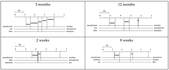
Figure 1.
CD diagram of the mean absolute percentage error. Note: transformer = transformer, tcn = Temporal Convolutional Network, lstm = long short-term memory, encDec = LSTM encoder–decoder, arimaxCorr = SARIMAX, transEnc = encoder transformer.
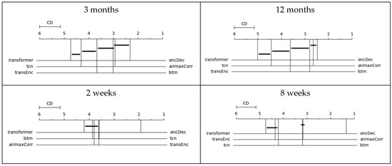
Figure 2.
CD diagram of the mean absolute error. Note: transformer = transformer, tcn = Temporal Convolutional Network, lstm = long short-term memory, encDec = LSTM encoder–decoder, arimaxCorr = SARIMAX, transEnc = encoder transformer.
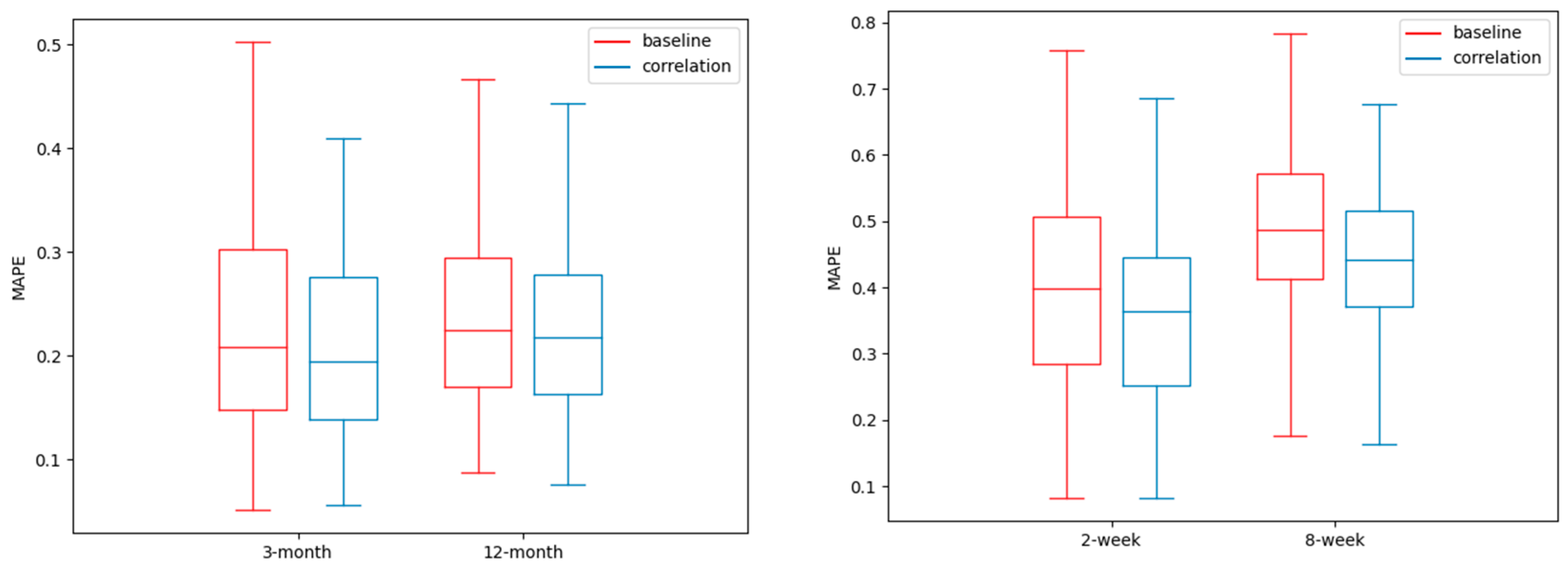
In Figure 3, it is possible to analyze the performance metrics between regions and at the same time show the contribution of the spatial–temporal correlation. The box plots of this figure show the average MAPE for the 82 regions of the LSTM encoder–decoder that includes the spatial–temporal correlation and a baseline LSTM encoder–decoder that does not include the spatial–temporal correlation. We can obtain two main findings from these graphs. First, the incorporation of the spatial–temporal correlation, as we conducted, improves the performance, because the box plots tend to show lower MAPE values for the monthly and weekly predictions. The second finding is the high variability in the error prediction between regions, regardless of the spatial–temporal correlation. For example, for the forecasting of three months, the MAPE varies from 0.05 to more than 0.4. There are regions with acceptable values of the MAPE and others with high values, for any of the forecasting horizons.
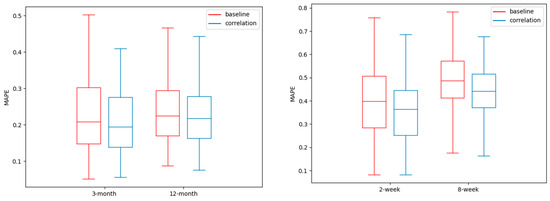
Figure 3.
The average MAPE of the regions, according to the LSTM encoder–decoder with and without (baseline) spatial–temporal correlation.
Finally, to understand the difference in performance between models, we categorized them into four percentile groups according to the MAPE and calculated the average of four features of the time series by group. Table 2 shows that in percentile 25 of the best-performing regions, the time series has a stronger trend, less variability, and a higher crime count. The feature named mean, which is the mean of crimes per period, suggests that the time series are less predictable in regions with fewer crimes. When the non-linearity feature is analyzed, it is clear that in the weekly time series, the best performance appeared in the less non-linear time series, but in the monthly time series, there is not a clear tendency to hold this finding.
Table 2.
Features of times series according to percentile of performance.
5. Conclusions
The best alternative model to predict the number of crimes in multiple regions was the LSTM encoder–decoder. The proposal model gave the best results for monthly and weekly predictions based on the MAE and MAPE metrics. Our methodology to incorporate the spatial–temporal correlation to the models contributes to the reduction in prediction error.
The models should improve because they were more efficient at predicting the crimes in the more dangerous regions; meanwhile, in the regions where the number of crimes is lower, and zero appears more frequently, the performance decays. This kind of time series tends to be more non-linear and has a weaker trend and high variability.
Future studies should examine the effectiveness of various approaches for capturing spatial–temporal correlations and examine the convenience of predicting the occurrence of a crime in a spatio-temporal range, instead of predicting the number of crimes in regions with low numbers of crimes. More complex methods generated in the state of the art, e.g., refs. [9,15], to predict the number of crimes at the hourly level should be compared with simple methods such as the LSTM encoder–decoder to predict the number of crimes in months or weeks. We have shown that more complex architectures like TCNs or transformers obtained worse results than more simple architectures, but new findings require a deep comprehension of the models’ behavior.
Author Contributions
Conceptualization, M.S. and L.-A.C.-V.; methodology, M.S. and L.-A.C.-V.; software, M.S.; validation, M.S.; formal analysis, M.S.; investigation, M.S. and L.-A.C.-V.; resources, M.S.; data curation, M.S.; writing—original draft preparation, M.S.; writing—review and editing, M.S. and L.-A.C.-V.; visualization, M.S.; supervision, M.S. All authors have read and agreed to the published version of the manuscript.
Funding
This manuscript comes from the Research Project Crime forecasting models of Costa Rica, supported by Technological Institute of Costa Rica. However, no external funding was received.
Institutional Review Board Statement
Not applicable.
Informed Consent Statement
Not applicable.
Data Availability Statement
Datasets are available at https://github.com/martin12cr/crimeCR. These datasets show the number of crimes that occurred in the 83 sub-areas of Costa Rica, named cantones.
Conflicts of Interest
The authors declare no conflicts of interest.
References
- Butt, U.M.; Letchmunan, S.; Hassan, F.H.; Koh, T.W. Hybrid of deep learning and exponential smoothing for enhancing crime forecasting accuracy. PLoS ONE 2022, 17, e0274172. [Google Scholar] [CrossRef] [PubMed]
- Meijer, A.; Wessels, M. Predictive Policing: Review of Benefits and Drawbacks. Int. J. Public Adm. 2019, 42, 1031–1039. [Google Scholar] [CrossRef]
- Kounadi, O.; Ristea, A.; Araujo, A.; Leitner, M. A systematic review on spatial crime forecasting. Crime Sci. 2020, 9, 7. [Google Scholar] [CrossRef] [PubMed]
- Solís, M.; Calvo-Valverde, L.-A. Performance of Deep Learning models with transfer learning for multiple-step-ahead forecasts in monthly time series. Intel. Artif. 2022, 25, 110–125. [Google Scholar] [CrossRef]
- Solís, M.; Calvo-Valverde, L.-A. A Proposal of Transfer Learning for Monthly Macroeconomic Time Series Forecast. Eng. Proc. 2023, 39, 58. [Google Scholar] [CrossRef]
- Mariano-Hernández, D.; Hernández-Callejo, L.; Solís, M.; Zorita-Lamadrid, A.; Duque-Perez, O.; Gonzalez-Morales, L.; Santos-García, F. A Data-Driven Forecasting Strategy to Predict Continuous Hourly Energy Demand in Smart Buildings. Appl. Sci. 2021, 11, 7886. [Google Scholar] [CrossRef]
- Alghamdi, J.; Huang, Z. Modeling Daily Crime Events Prediction Using Seq2Seq Architecture. In Databases Theory and Applications, Proceedings of the 32nd Australasian Database Conference, ADC 2021, Dunedin, New Zealand, 29 January–5 February 2021; Springer: Cham, Switzerland, 2021; pp. 192–203. [Google Scholar] [CrossRef]
- Anuvarshini, S.R.; Deeksha, N.; Deeksha, S.C.; Krishna, S.K. Crime Forecasting : A Theoretical Approach. In Proceedings of the 2022 IEEE 7th International Conference on Recent Advances and Innovations in Engineering (ICRAIE), Mangalore, India, 1–3 December 2022. [Google Scholar] [CrossRef]
- Dong, Q.; Li, Y.; Zheng, Z.; Wang, X.; Li, G. ST3DNetCrime: Improved ST-3DNet Model for Crime Prediction at Fine Spatial Temporal Scales. ISPRS Int. J. Geo-Inf. 2022, 11, 529. [Google Scholar] [CrossRef]
- Sharmin, S.; Alam, F.I.; Das, A.; Uddin, R. An Investigation into Crime Forecast Using Auto ARIMA and Stacked LSTM. In Proceedings of the 2022 International Conference on Innovations in Science, Engineering and Technology (ICISET), Chittagong, Bangladesh, 26–27 February 2022. [Google Scholar] [CrossRef]
- Ibrahim, N.; Wang, S.; Zhao, B. Spatiotemporal Crime Hotspots Analysis and Crime Occurrence Prediction. In Advanced Data Mining and Applications, Proceedings of the 15th International Conference, ADMA 2019, Dalian, China, 21–23 November 2019; Lecture Notes in Computer Science; Springer: Cham, Switzerland, 2019; pp. 579–588. [Google Scholar] [CrossRef]
- Stec, A.; Klabjan, D. Forecasting crime with deep learning. arXiv 2018, arXiv:1806.01486. [Google Scholar]
- Stalidis, P.; Semertzidis, T.; Daras, P. Examining Deep Learning Architectures for Crime Classification and Prediction. Forecasting 2021, 3, 741–762. [Google Scholar] [CrossRef]
- Rayhan, Y.; Hashem, T. AIST: An Interpretable Attention-Based Deep Learning Model for Crime Prediction. ACM Trans. Spat. Algorithms Syst. 2023, 9, 1–31. [Google Scholar] [CrossRef]
- Hu, K.; Li, L.; Liu, J.; Sun, D. DuroNet. ACM Trans. Internet Technol. 2021, 21, 1–24. [Google Scholar] [CrossRef]
- Cruz-Nájera, M.A.; Treviño-Berrones, M.G.; Ponce-Flores, M.P.; Terán-Villanueva, J.D.; Castán-Rocha, J.A.; Ibarra-Martínez, S.; Santiago, A.; Laria-Menchaca, J. Short Time Series Forecasting: Recommended Methods and Techniques. Symmetry 2022, 14, 1231. [Google Scholar] [CrossRef]
- Herbold, S. Autorank: A Python package for automated ranking of classifiers. J. Open Source Softw. 2020, 5, 2173. [Google Scholar] [CrossRef]
Disclaimer/Publisher’s Note: The statements, opinions and data contained in all publications are solely those of the individual author(s) and contributor(s) and not of MDPI and/or the editor(s). MDPI and/or the editor(s) disclaim responsibility for any injury to people or property resulting from any ideas, methods, instructions or products referred to in the content. |
© 2024 by the authors. Licensee MDPI, Basel, Switzerland. This article is an open access article distributed under the terms and conditions of the Creative Commons Attribution (CC BY) license (https://creativecommons.org/licenses/by/4.0/).