Deterministic Design Procedures on Limited Field-of-View Planar Arrays for Satellite Communications Employing Aperture Scaling ^†

Abstract

The antenna field of view, the angle range that can be accessed by scanning the main beam of a phased array, is one of the key performance prescriptions especially for space-borne aerials. The classical example of the full Earth, continental and subcontinental field of view of the geosynchronous satellite is indicative, and it extends to the medium and lower orbit multibeam telecommunication systems. There, a high-gain, very small beamwidth pencil beam should scan a given service area. At the same time, it should exhibit extremely low sidelobes in order not to present interference to adjacent geographical areas, served by neighboring beams, and keep its grating lobes out of the Earth’s surface. High-throughput telecommunication satellites should comply with those prescriptions to be given permission for placement in orbit. Thus, the motivation for delivering solid methods for the design of limited-field-of-view array antennas is high. A proposal in this direction is presented in the work at hand. Indeed, in the present study a scaling transformation is used to map a wide-angle scanning array to a limited-field-of-view one. We start the design from a Full-Field-of-View array with the appropriate half-power beamwidth, sidelobe level, and directivity index, and then we enlarge it to attain the desired one with the limited-field-of-view pattern characteristics. The potential of the method is solid since it augments the limited-field-of-view design methods using the excellent performance of the respective full-field-of-view ones. As a result, the synthesis of a limited-field-of-view array can use any of the well-known array synthesis methods in conjunction with the right scaling. Additionally, one can employ design methods that rely on sampling of planar aperture distributions. Various design examples, employing both sampling of continuous apertures and utilizing classical full-field-of-view array synthesis methods, are included and presented in detail, verifying the merit of our approach.

1. Introduction

Most of the antenna arrays are designed for wide-angle (full field-of-view (FFoV)) scanning. However, there are antenna systems that operate fulfilling certain restrictions in limited scan coverage. Radiating equipment with limited-field-of-view (LFoV) antennas is usually incorporated in space-borne systems for satellite communications [1,2,3].

Conventional design of these antennas follows two steps. In the first step a judicious choice of the size of the radiating aperture and the accompanying continuous excitation is made. The choice is the one that exhibits far-field indexes that are closer to the design requirements. Tabulated data such as those presented, for example, in Table 1.2 of [4], can be very helpful during this step. In the second step, the chosen continuous excitation is sampled to produce a space tapering that achieves approximately the same far-field performance. The sampling can follow deterministic or even stochastic routes [4,5,6,7,8,9,10,11]. Admittedly, those methods give adequate practical solutions but somehow are rather limited in number, and also lack the degree of control in the final result (the far-field pattern and its indices) when compared to the ones developed for the full field of view.

The key point of our work is the use of the scaling transformation that makes it possible to map FFoV designs to LFoV ones. Thus, the current study, apart from introducing design procedures to cope with arrays with restriction in the scan coverage, focuses on transforming solutions by using a scaling transformation that produces LFoV systems after borrowing developed designs from the FFoV set. It must be noted that we can use any of the well-known array synthesis methods, like Dolph–Chebyshev [12], Villeneuve [13], Orchard [14], and orthogonal [15], while design methods which are based on sampling of planar aperture distributions, like parabolic, truncated Gaussian [16], Hansen [17,18], Taylor [19] and Bayliss [20], are also applicable.

The paper is structured as follows. In Section 2, the scaling transformation is analyzed and the employed design procedure is presented. Detailed representative design examples, which verify the potential of the method, are given in Section 3. The overall evaluation of the method is discussed in the conclusions.

2. Materials and Methods

In the current section, the scaling transformation and the respective design procedure are presented.

2.1. Scaling Transformation

We assume a radiating aperture of surface S on the xy plane, having an excitation distribution $I\left(x/\sqrt{S},y/\sqrt{S}\right)$. The respective far-field pattern reads:

$$AF\left(\varphi ,\theta \right)={\displaystyle \underset{Aperture}{\iint }I\left(x/\sqrt{S},y/\sqrt{S}\right)\exp \left(-j\frac{2\pi }{\lambda }\left(x\cos \varphi \sin \theta +y\sin \varphi \sin \theta \right)\right)dxdy}.$$

(1)

If we substitute in (1):

$$\zeta =x/\sqrt{S};\hspace{1em}\xi =y/\sqrt{S},$$

(2)

we have:

$$AF\left(\varphi ,\theta \right)={\displaystyle \underset{Aperture}{\iint }I\left(\zeta ,\xi \right)\exp \left(-j\frac{2\pi }{\lambda }\left(\zeta \cos \varphi +\xi \sin \varphi \right)\sqrt{S}\sin \theta \right)d\xi d\zeta }.$$

(3)

From (1) and (3), it is obvious that the relation between real space and the observation angle θ is solely included in the term $\left(2\pi /\lambda \right)\sqrt{S}\sin \theta =\beta \sqrt{S}\sin \theta$:

$$AF\left(\varphi ,\theta \right)=f\left(\beta \sqrt{S}\sin \theta \cos \varphi ,\beta \sqrt{S}\sin \theta \sin \varphi \right).$$

(4)

As a result, if we apply a scaling procedure, mapping the geometry (x,y) to (x′,y′), then the observed field in the angle θ is moved to angle θ’. The equivalence relation is given by the following:

$$r\sin \theta =r^{\prime }\sin {\theta }^{\prime }\iff {\theta }^{\prime }={\sin }^{-1}\left(r\sin \theta /r^{\prime }\right),$$

(5)

where r and r′ are the distances of a point from the center of the aperture in the initial and scaled cases. Equivalently, one can reach a relation:

$$\begin{array}{l}xu=x^{\prime }{u}^{\prime }\iff x\cos \left(\varphi \right)\sin \left(\theta \right)=x^{\prime }\cos \left(\varphi \right)\sin \left({\theta }^{\prime }\right)\\ yv=y^{\prime }{v}^{\prime }\iff y\sin \left(\varphi \right)\sin \left(\theta \right)=y^{\prime }\sin \left(\varphi \right)\sin \left({\theta }^{\prime }\right)\end{array}.$$

(6)

The previous equation suggests that an up-scaling in real space (up-scaling the continuous or discrete aperture) results in shrinking (following a reciprocal scaling law) of the u-v space in such a way that previously invisible (having imaginary u and v) regions are entering the visible unit circle.

It is noticed that the above given formulation holds not only for planar apertures, but also for line sources (see Figure 1). For a line source of length L, instead of (1) and (3), now it is:

$$\begin{array}{l}AF\left(\varphi ,\theta \right)={\displaystyle \underset{x=-L/2}{\overset{x=+L/2}{\int }}I\left(x/\left(L/2\right)\right)\exp \left(-j2\pi \left(x\sin \theta \right)\right)dx}=\left(L/2\right){\displaystyle \underset{-1/2}{\overset{+1/2}{\int }}I\left(\zeta \right)\exp \left(-j2\pi \left(L/2\right)\sin \theta \zeta \right)d\zeta }\\ \zeta =x/\left(L/2\right)\end{array}.$$

(7)

The first pictorial example for comprehension reasons is given next for a linear array, which is a case of line source. Indeed, we use a line source of length L = 3λ with the following excitation:

$$I\left(x/\left(L/2\right)\right)={\displaystyle \sum _{v=-3}^{+3}\delta \left(x/\left(L/2\right)-v/3\right)},$$

(8)

where δ is the Dirac Delta function. Equation (8) represents a uniformly excited linear array of 7 point sources in equidistance d = 0.5λ. Using a scaling factor of μ = 2, we reach a new array with d = 1λ, where the field-of-view range is limited to ${\theta }_0={\sin }^{-1}\left(\sin \left(\pi /2\right)/\mu \right)={\sin }^{-1}\left(0.5\right)=30°$.

It is obvious that the initial pattern is compressed, as the [0, 90°] visible region is shrunk to the new one [0, 30°]. Additionally, the half-power beamwidth, (HPBW) decreases from ~7.3° degrees to ~3.6°.

Based on Relation (5), one can formulate a mapping between FFoV and LFoV systems. This mapping, which is derived next, apart from the transform in Equation (5), includes the following:

• Scaling factor equation (Equation (9));
• HPBW equation (Equation (10));
• Directivity equation (Equation (18));
• Sidelobe level (SLL).

To construct the mapping, first, the scaling factor, μ, must be computed. Assuming that the field-of-view range is scaled down from π/2 (the full-field-of-view range) to θ₀ (the limited-field-of-view range), then using (5) we reach the following equation (scaling factor equation):

$$\mu ={\displaystyle \frac{r_L}{r_F}}=\sin {\displaystyle \frac{\pi }{2}}/\sin {\theta }_0\ge 1,$$

(9)

where subscript F stands for FFoV while subscript L stands for LFoV systems.

Then, given the HPBW_L equation (Equation (5)), we can determine the HPBW_F. In the current work, we focus on broadside beams where $sin\left(\theta \right)\cong \theta$ practically holds. As a result, the HPΒW equation reads:

$$HPB{W}_L={\displaystyle \frac{r_F}{r_L}}\cdot HPB{W}_F={\displaystyle \frac{1}{\mu }}\cdot HPB{W}_F.$$

(10)

Apart from the previous equations, a relation between the directivities of the two designs exists. This is made possible if the radiating elements of the LFoV case have the following radiation pattern:

$$EP({\theta }^{\prime })=\left\{\begin{array}{cc}1& {\theta }^{\prime }\le {\theta }_0\\ 0& {\theta }_0<{\theta }^{\prime }\end{array}\right..$$

(11)

We start from the directivity of the FFoV array:

$$D_F=4\pi {\left({\displaystyle \underset{0}{\overset{2\pi }{\int }}{\displaystyle \underset{0}{\overset{\overline{\theta }=\pi /2}{\int }}{\left|AF\left(\cos \varphi \sqrt{S}\sin \theta ,\sin \varphi \sqrt{S}\sin \theta \right)\right|}^2\sin \theta d\varphi d\theta }}\right)}^{-1}.$$

(12)

Now, enforcing a transformation from variable θ to θ′, using (5) we have:

$$\theta ={\sin }^{-1}\left({\displaystyle \frac{r^{\prime }\sin {\theta }^{\prime }}{r}}\right)={\sin }^{-1}\left(\mu \sin {\theta }^{\prime }\right);\hspace{1em}d\theta =d{\theta }^{\prime }\mu {\displaystyle \frac{\cos {\theta }^{\prime }}{\cos \theta }}.$$

(13)

The directivity index after some algebra is given below:

$$D_F={\displaystyle \frac{4\pi }{{\mu }^2}}\cdot {\left({\displaystyle \underset{0}{\overset{2\pi }{\int }}{\displaystyle \underset{0}{\overset{\overline{{\theta }^{\prime }}={\sin }^{-1}\left(\frac{1}{\mu }\sin (\pi /2)\right)}{\int }}{\left|AF\left(\cos \varphi \sqrt{S^{\prime }}\sin {\theta }^{\prime },\sin \varphi \sqrt{S^{\prime }}\sin {\theta }^{\prime }\right)\right|}^2\sin {\theta }^{\prime }d\varphi d{\theta }^{\prime }\left(\frac{\cos {\theta }^{\prime }}{\cos \theta }\right)}}\right)}^{-1}.$$

(14)

Figure 2 depicts cosθ/cosθ′ = cosθ_F/cosθ_L (blue curves) for μ = (5, 6, 7, 8, 9, 10). The vertical red lines depict the upper border of the LFoV range, $\left[{\sin }^{-1}\left({\displaystyle \frac{1}{\mu }}\sin \left(\pi /2\right)\right)\right]$. Increasing μ, we move the border to the left.

Note that for scaling factors at least higher than 5 in the LFoV range, the following approximation holds:

$$\cos {\theta }^{\prime }/\cos \theta \approx 1.$$

(15)

So, (14) results in:

$$.D_F\approx {\displaystyle \frac{4\pi }{{\mu }^2}}\cdot {\left({\displaystyle \underset{0}{\overset{2\pi }{\int }}{\displaystyle \underset{0}{\overset{\overline{\theta }={\sin }^{-1}\left(\frac{1}{\mu }\sin \left(\pi /2\right)\right)}{\int }}{\left|AF\left(\cos \varphi \sqrt{S^{\prime }}\sin {\theta }^{\prime },\sin \varphi \sqrt{S^{\prime }}\sin {\theta }^{\prime }\right)\right|}^2\sin {\theta }^{\prime }d\varphi d{\theta }^{\prime }}}\right)}^{-1}$$

(16)

If we assume that we use radiating elements with the pattern given by (11) for the LFoV case, the corresponding directivity takes the following form:

$$.D_L=4\pi {\left({\displaystyle \underset{0}{\overset{2\pi }{\int }}{\displaystyle \underset{0}{\overset{\overline{{\theta }^{\prime }}}{\int }}{\left|AF\left(\cos \varphi \sqrt{S^{\prime }}\sin {\theta }^{\prime },\sin \varphi \sqrt{S^{\prime }}\sin {\theta }^{\prime }\right)\right|}^2\sin {\theta }^{\prime }d\varphi d{\theta }^{\prime }}}\right)}^{-1}$$

(17)

Equations (16) and (17) result in the directivity equation:

$$D_F={\displaystyle \frac{1}{{\mu }^2}}{D}_L\Rightarrow D_{\begin{array}{l}LFoV with\hspace{1em}Brick\hspace{1em}Wall\hspace{1em}Element\\ Pattern\end{array}}\left(dBi\right)=10{\log }_{10}{\mu }^2+D_{\begin{array}{l}FFoV with\hspace{1em}Omni\hspace{1em}Element\\ Pattern\end{array}}\left(dBi\right).$$

(18)

Note that, for example, for a scaling factor of μ = 7, the previous expression gives a boost of approximately 16.9 dB in the directivity of the LFoV design.

Last, as far as the SLL is concerned, it remains constant between the two designs, since the scaling transformation varies the angle of view but not the amplitude of the field.

The transformation results are gathered in

Table 1. The mapping between LFoV and FFoV design requirements.

LFoV Prescription	Scaling Transform Equation	FFoV Prescription
From 0 to θ0	$\left({\displaystyle \frac{r_L}{r_F}}\right)={\displaystyle \frac{\sin (\pi /2)}{\sin ({\theta }_0)}}$	From 0 to π/2
HPBWL	$HPB{W}_F\cong {\left({\displaystyle \frac{r_L}{r_F}}\right)}^{1}HPB{W}_L$	HPBWF
SLLL	$SL{L}_F=SL{L}_L$	SLLF
DL	$D_F=10{\log }_{10}{\left({\displaystyle \frac{r_F}{r_L}}\right)}^2+D_L$	DF

.

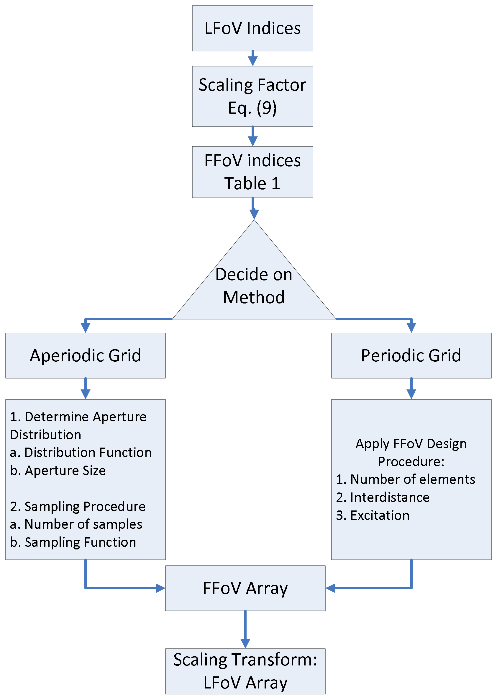
2.2. Design Procedure

A design procedure for narrow-beam low-sidelobe designs is given in this section. The successive steps are listed in the flowchart of Figure 3.

The problem is defined by the statement of the LFoV prescriptions. After that, the scaling factor and the FFoV indices can be computed. Next, the designer has to choose either an aperiodic or a periodic grid for the array layout.

In the first case, the aperture distributions have to be determined along with the aperture size. Next, a sampling procedure follows that is defined by the number of samples and the chosen sampling function.

In the second case, in order for a FFoV design procedure to be used, the number of elements, the interelement distance, and the element excitation are determined. After that, the FFoV array is produced and, by enforcing the inverse scaling transform, we end up with an array that complies with the LFoV prescriptions. Detailed design examples are given in the next section.

3. Results

The design examples are drawn from the following two different sets of FFoV solutions:

• Sampling of continuous apertures;
• Use of FFoV array synthesis methods.

In the first case, the prescriptions (all but the LFoV) are used to design a FFoV continuous illuminated aperture (meaning the aperture distribution is determined as done in Step 3 of examples A.1 and A.2). Subsequently, we need to produce an array out of the continuous aperture (sampling procedure) by properly sampling the later. The sampling entails the element radiator size determination (via the grating lobe constraint) and the size of the elements (via the directivity constraint), embodied in Step 4 of examples A.1 and A.2. At this point, a FFoV array is produced, Thus, finally, the scaling transformation should be employed to acquire the final LFoV array. This can be trivial (example A.1), or more elaborate, like radial wrapping (example A.2). In the second case, first a FFoV array is constructed, following the classical FFoV method, that results in an acceptable array (element type, placement, and excitation presented in Step 3 of examples B.1 and B.2) complying with the FFoV indices, (SLL_F, HPBW_F, and D_F). Subsequently, again the scaling transformation is invoked to acquire the array complying with the initial LFoV constraint.

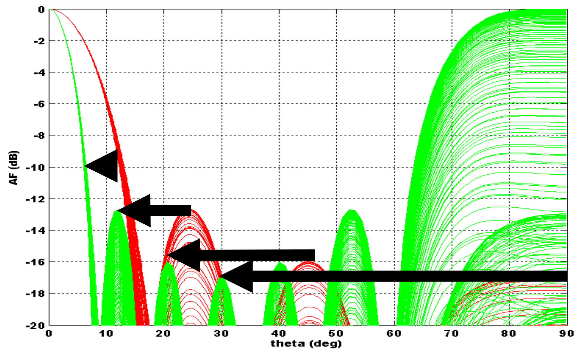
3.1. Sampling of Continuous Apertures

It is well known that continuous apertures and arrays can share similar characteristics and an antenna array can be given by sampling an aperture. To have an aperture or an array with a desired LFoV, we must extend the design in the appropriate enlargement.

The procedure incorporates the following steps:

• The scaling factor is derived from the range of view.
• The FFoV indices SLL_F, HPBW_F, and D_F are derived from the LFoV ones.
• The aperture distribution for the FFoV is found.
• A sampling procedure is followed to transform the continuous distribution to an array.
• The scaling transformation is enforced on the array to produce the final result.

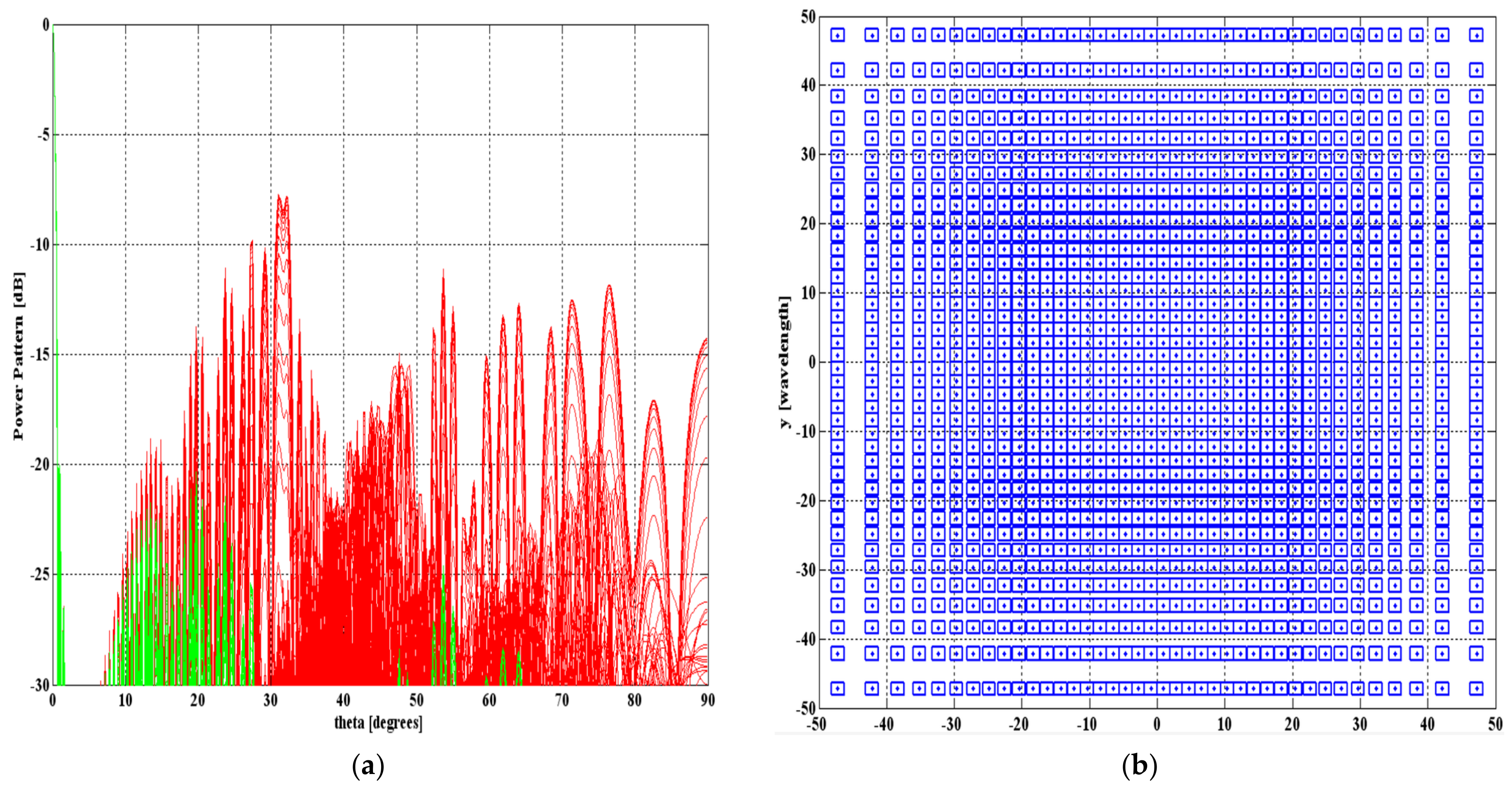
3.1.1. Example A.1

We produce an array that is a linear x-axis array with linear y-axis arrays as elements. The final planar array should be square and should use the same space taper in both the x- and in y-axes. With such an array, the 2D design is reduced to a 1D design.

The limited-field-of-view indices are SLL_L < −20 dB, HPBW_L~1.2°, and D_L > 48 dBi with θ₀~8°. Let us now follow the steps of the proposed design procedure:

Step 1: The scaling factor is equal to 7.

Step 2: Using Table 1, the respective FFoV indices are SLL_F < −20 dB, HPBW_F~8.4°, D_F > 31 dBi.

Step 3: In this step, the aperture distribution and the size of the aperture are determined from the FFoV indices. We use a (cosθ)ⁿ distribution for the linear array, and from the SLL_F we determine the exponent n. This is done as follows: From Table 1.1 of [4], we copy that for SLL = [−13.2, −23, −32] and the respective n takes the values n = [0, 1, 2]. Using interpolation for SLL_F = −20 dB, we find n~0.694. Then, from HPBW_F, we determine the length of the linear aperture of the FFoV linear array. Indeed, again from Table 1.1 of [1], we copy that for n = [0, 1, 2], which is HPBW = [50.8, 68.8, 83.2]/(aperture length in wavelengths). Thus, using interpolation for n~0.694 (the previously determined exponent), we obtain HPBW_F~63.29/(aperture length in wavelengths). Thus, solving for the aperture length of the FFoV array, we find that it is approximately equal to 7.53λ.

Step 4: In order to determine the sampling procedure, we need to determine the number of elements and choose a proper array element placement procedure. We start from the determination of the number and size of the elements. If the nearest distance between the array elements [21] is ε, then the noise-like pattern [22] (~inversely proportional to the number of the elements of the array), starts from the first grating lobe. The formula is [23]:

$$|u|={\displaystyle \frac{3.8}{k\cdot \epsilon }},$$

(19)

where k is equal to 2π and ε is measured in wavelengths. By equating u as the sine of the field of view we get:

$$\sin (FoV)={\displaystyle \frac{3.8}{k\cdot \epsilon }}$$

(20)

From (20), the minimum distance between the elements can be determined. We use elements that cover all the available space [24], since their patterns should approximate the brick-wall function (Equation (11)). From the above, we can proceed to the determination of the element directivity, assuming square, uniformly illuminated elements:

$$D_e=4\pi S^2\Rightarrow D_e=4\pi {\left(2\cdot \epsilon \right)}^2.$$

(21)

Then from [1]:

$$D_L=N_e\cdot D_e,$$

(22)

we can find the number of elements. Taking into account that the square of the number of elements should be an integer (since we aim at a square array), the result is approximately equal to N_e = 1600.

Thus, now that we have determined the number of elements, we can use the procedure described in [23] (p. 582) to design the linear array.

Step 5. Last, we scale the design to produce the final array. Although we have determined the size of the elements from the previous step, we must avoid any possible overlapping between the elements. Thus, the side-length s takes the minimum value (multiplied, of course, by the scaling factor) between ε and the minimum inter-distance of adjacent elements. The final array has 1600 elements of s = 1.86λ. The final array layout and power pattern are given in Figure 4. The achieved directivity is equal to D = 48.50 dBi.

3.1.2. Example A.2

We produce a LFoV array employing the radial wrapping technique [25]. The prescribed indices are SLL_L < −20 dB, HPBW_L~0.6°, and D_L > 50 dBi with θ₀~8°. Let us now follow the steps of the proposed design procedure:

Step 1: The scaling factor is equal to 7.

Step 2: Using Table 1, the respective FFoV indices are SLL_F < −20 dB, HPBW_F~4.2°, and D_F > 33.1 dBi.

Step 3: Now the aperture distribution should be determined from the FFoV indices.

We use a paraboloidal distribution for a circular-aperture array and from the SLL we determine the exponent n. From Table 1.2 of [4], we copy that for SLL = [−17.6, −24.6, −30.6] and the respective n takes the values n = [0, 1, 2]. Using interpolation for SLL_F = −20 dB, we find n~0.34. Additionally, from HPBW_F, we determine the radius of the FFoV circular-aperture array. Indeed, again from Table 1.2 of [4], we copy that for n = [0, 1, 2], and it is HPBW = [58.9, 72.7, 84.3]/(circular-aperture diameter in wavelengths). Thus, using interpolation, we obtain HPBW_F~63.63/(circular-aperture diameter in wavelengths). Now, solving for the circular-aperture diameter of the FFoV array, we find that it is approximately equal to 15.15λ, and thus the respective diameter of the LFoV array is μ times bigger. This parameter is used in the next step by the radial wrapping technique to determine the final result.

Step 4: In order to apply the sampling procedure, we need to determine the number of elements and choose a proper array element placement method. We start from the determination of the number and size of the elements.

Following the same path as in Step 3 of the previous example, we can find the number of elements N_e = 625 and an initial side-length equal to 3.59λ.

Before we can employ the radial wrapping, we should provide an initial uniform array. This is done as follows: From a regular square grid array having elements with inter-distance equal to λ/2, we use the elements that are inside a circular disc of radius R₀ = 5.47λ. This value of R₀ is determined so that the circular-aperture array has a number of elements approximately equal to the value determined previously. In this way, the number of elements is 640.

Next, we employ the procedure described in [25].

Step 5: Last, we employ the scaling transformation. The final layout is given in Figure 5 along with the achieved power pattern. The final side-length, s = 3.22λ, is determined as described in Step 5 of the previous example while D = 49.33 dBi. Note that, although the achieved directivity is slightly below the desired value, we present this example in order to show that at the end of the design procedure, a fine tuning, with respect to the number of the elements, may be appropriate.

Before we proceed to the next examples, a note is in order. Here, using paraboloidal functions to represent the aperture taper, we were able to contribute a closed form formula that provides the element placement. Indeed, an element whose center is initially placed at the point (r₁, φ) is finally placed at a point (r₂, φ), where for r₁ and r₂ the following holds:

$$r_2=\sqrt{1-\sqrt[n+1]{1-r_1^2}}.$$

(23)

The relative proof can be found in the Appendix A.

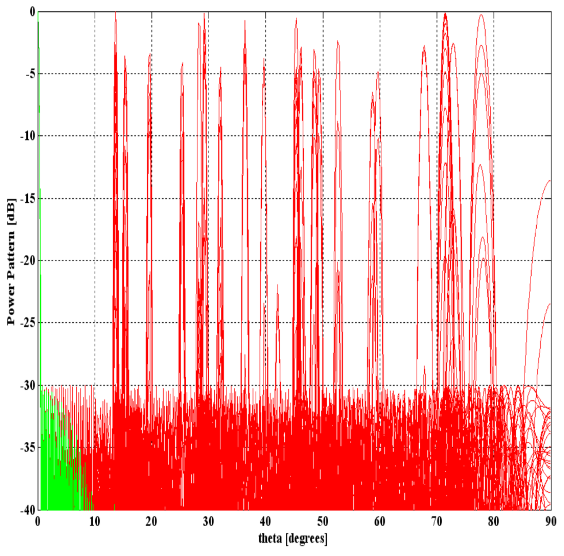
3.2. Use of FFoV Array Synthesis Methods

We proceed to design procedures that make use of FFoV array synthesis methods and we focus on square arrays. Such a procedure incorporates the following steps:

• The scaling factor is derived from the range of view;
• The FFoV indices SLL_F, HPBW_F, and D_F are derived from the LFoV ones;
• A FFoV array synthesis method is used to provide the FFoV solution;
• The scaling transformation is enforced on the array to produce the final result.

3.2.1. Example B.1

In the first example, we combine two identical Dolph–Chebyshev linear arrays placed in x- and y-axes and, using pattern multiplication [23], we produce a square planar array. This results in a pattern that has lower sidelobes than those specified in all planes, except the principal ones along the axes. Furthermore, the planar array design is limited from 2D to 1D.

The limited-field-of-view indices are SLL_L < −30 dB, HPBW_L~0.4°, and D_L > 50 dBi and the range of view is ~10°. Let us now follow the Steps 1 to 4:

Step 1: The scaling factor is found to be approximately equal to 5.76.

Step 2: The FFoV indices are SLLF < −30 dB, HPBW_F ~2.3°, and D_F > 35 dBi.

Step 3: To design the FFoV array, we need the interelement distance, the number of the elements, and the excitation. Since the excitations are separable, then with good approximation the following holds [1]:

$$D_F=\pi \cdot D_x\cdot D_y=\pi \cdot D^2\Rightarrow D=\sqrt{D_F/\pi }\Rightarrow D=15dBi,$$

(24)

where D_x = D_y = D is the directivity of a single FFoV linear array. From the beam-broadening factor of a Chebychev array with SLL = −30 dB, a directivity of 15 dBi is achieved by 37 elements (d = λ/2). This gives D_1F = 35.1 dBi and HPBW_F = 2 × 1.685°. We scale the inter-distance d of the elements to achieve the prescribed HPBW. Then the directivity becomes D_2F = 38.34 dBi.

Step 4: The scaling transformation provides the final array, where we use elements of side-length equal to μ × d to achieve a near brick-wall pattern [26]. The achieved power pattern is given in Figure 6. The directivity of the array is 53.72 dBi. Note here that we obtain 3 dB above the prescribed lower bound of D_L due to D_2F−D_1F~3 dB (this is a result of the effort to achieve the prescribed HPBW_F).

3.2.2. Example B.2

In our second example, we use a technique on a square array to produce equal sidelobes in all constant φ cuts around the array.

The LFoV indices are SLL_L < −25 dB, HPBW_L~1°, and D_L > 42 dBi and the range of view is ~10°. Let us now follow the steps of the proposed design procedure:

Step 1: The scaling factor is found to be approximately equal to 5.76.

Step 2: The respective FFoV indices are: SLL_F < −25 dB, HPBW_F~5.76°, and D_F > 26.8 dBi.

Step 3: Next, we apply the FFoV design method. To design the array, we need the interelement distance, the number of the elements, and the excitation.

The number of elements is determined by [4]:

$$D_F=e_T{N}_e{D}_e\Rightarrow N_e=D_F/(e_T{D}_e),$$

(25)

where D_e is the average element directivity (gain divided by loss efficiency) and e_T is the taper efficiency. We assume that e_T = 1/2 and D_e is equal to the isolated element directivity since we aim at approximately estimating the number of elements of the array. We also assume that the radiating elements are placed in a λ/2 × λ/2 lattice in the FFoV array and also that they are uniformly illuminated squares (λ/2 × λ/2). D_e is then equal to π. Applying (25), we find that N_e = 17.62. Thus, since we are going to design a square array, we choose the value of 18 × 18 for the number of the elements.

The excitation for the 18 × 18 array is computed following [27] and using the SLL_F prescription. For this array, the HPBW is 1.14 times greater than the prescribed FFoV one, which is equal to ~5.7°. Thus, we set the inter-distance equal to d = (1/2) × 1.14.

Step 4: Using the scaling transformation, the final array produces the power pattern given in Figure 7. The respective directivity is D_L = 44.44 dBi for elements with side-length equal to μ × d.

4. Conclusions

A study for the deterministic synthesis of LFoV planar arrays is presented. The procedure is implemented through the initial design of a FFoV case with the prescribed HPBW and SLL, and a desired directivity index. The next step comprises a scaling transformation, which results in a new enlarged array characterized by the same SLL, shrunk HPBW, and increased directivity. Design examples of both non-uniformly/uniformly excited periodic/aperiodic arrays verify the applicability of the proposed method. The presented procedure forms a communicating path between LFoV and FFoV design methods. In this way, it provides the means to shape the far-field pattern, in a finite angular range near the main beam, either following classical array synthesis methods or employing proper sampling on planar aperture distributions.

Furthermore, since the proposed synthesis is deterministic, it can provide benchmark solutions or, preferably, be integrated into various stochastic methods [28], to initiate optimized solutions to practical [29] design problems.

References

- Kaifas, T.N.; Samaras, T.; Siakavara, K.; Sahalos, J.N. A UTD-OM technique to design slot arrays on a perfectly conducting paraboloid. IEEE Trans. Antennas Propag. 2005, 53, 1688–1698. [Google Scholar] [CrossRef]
- Kaifas, T.N.; Sahalos, J.N. Design and Performance Aspects of an Adaptive Cylindrical Beamforming Array. IEEE Antennas Propag. Mag. 2012, 54, 51–65. [Google Scholar] [CrossRef]
- Kaifas, T.N.; Siakavara, K.; Vafiadis, E.; Samaras, T.; Sahalos, J.N. On the design of conformal slot arrays on a perfectly conducting elliptic cone. Electr. Eng. 2006, 89, 95–105. [Google Scholar] [CrossRef]
- Milligan, T.A. Space tapered circular (ring) array. IEEE Antennas Propag. Mag. 2004, 46, 70–73. [Google Scholar] [CrossRef]
- Skolnik, M.I.; Sherman, J.W.; Ogg, F.C. Statistically Designed Density-Tapered Arrays. IEEE Trans Antennas Propag. 1964, 12, 408–409. [Google Scholar] [CrossRef]
- Kaifas, T.N.; Babas, D.G.; Toso, G.; Sahalos, J.N. Μultibeam Antennas for Global Satellite Coverage: Theory and Design. IET Microw. Antennas Propag. 2016, 10, 1475. [Google Scholar] [CrossRef]
- Kaifas, T.N. Direct radiating array design via convex aperture synthesis, pareto front theory, and deterministic sampling [antenna designer’s notebook]. IEEE Antennas Propag. Mag. 2014, 56, 134–151. [Google Scholar] [CrossRef]
- Kaifas, T.N.; Babas, D.G.; Miaris, G.S.; Vafiadis, E.E.; Siakavara, K.; Toso, G.; Sahalos, J.N. A Stochastic Study of Large Arrays Related to the Number of Electrically Large Aperture Radiators. IEEE Trans. Antennas Propag. 2014, 62, 3520–3533. [Google Scholar] [CrossRef]
- Kaifas, T.N.; Sahalos, J.N. On the Geometry Synthesis of Arrays with a Given Excitation by the Orthogonal Method. IEEE Trans. Antennas Propag. 2008, 56, 3680–3688. [Google Scholar] [CrossRef]
- Kaifas, T.N.; Babas, D.G.; Sahalos, J.N. Design of Planar Arrays with Reduced Nonuniform Excitation Subject to Constraints on the Resulting Pattern and the Directivity. IEEE Trans. Antennas Propag. 2009, 57, 2270–2278. [Google Scholar] [CrossRef]
- Kaifas, T.N.; Babas, D.G.; Miaris, G.S.; Siakavara, K.; Vafiadis, E.; Sahalos, J.N. Aperiodic Array Layout Optimization by the Constraint Relaxation Approach. IEEE Trans. Antennas Propag. 2012, 60, 148–163. [Google Scholar] [CrossRef]
- Dolph, C.L. A current distribution for broadside arrays which optimizes the relationship between beamwidth and sidelobe level. Proc. IRE 1946, 34, 335–348. [Google Scholar] [CrossRef]
- Villeneuve, T. Taylor patterns for discrete arrays. IEEE Trans. Antennas Propag. 1984, 32, 1089–1092. [Google Scholar] [CrossRef]
- Orchard, H.J.; Elliott, R.S.; Stern, G.J. Optimising the synthesis of shaped beam antenna patterns. IEE Proc. H (Microw. Antennas Propag.) 1985, 132, 63–68. [Google Scholar] [CrossRef]
- Sahalos, J.N. Orthogonal Methods for Array Synthesis: Theory & the ORAMA Computer Tool; Wiley: West Sussex, UK, 2006. [Google Scholar]
- Doundoulakis, G.; Gethin, S. Far field patterns of circular paraboloidal reflectors. In 1958 IRE International Convention Record; IEEE: New York, NY, USA, 1959; pp. 155–173. [Google Scholar] [CrossRef]
- Hansen, R.C. Circular aperture distribution with one parameter. Electron. Lett. 1975, 11, 184. [Google Scholar] [CrossRef]
- Hansen, R.C. A one-parameter circular aperture distribution with narrow beamwidth and low sidelobes. IEEE Trans Antennas Propag. 1976, 24, 477–480. [Google Scholar] [CrossRef]
- Taylor, T.T. Design of circular apertures for narrow beamwidth and low side lobes. IRE Trans Antennas Propag. 1960, 8, 17–22. [Google Scholar] [CrossRef]
- Bayliss, E.T. Design of monopulse antenna difference patterns with low sidelobes. Bell Syst. Tech. J. 1968, 47, 623–650. [Google Scholar] [CrossRef]
- Fante, R.L.; Robertshaw, G.A.; Zamoscianyk, S. Observation and Explanation of an Unusual Feature of Random Arrays with a nearest—Neighbor Constraint. IEEE Trans Antennas Propag. 1991, 39, 1047–1049. [Google Scholar] [CrossRef]
- Lo, Y.T. A mathematical theory of antenna arrays with randomly spaced elements. IEEE Trans. Antennas Propag. 1964, 12, 257–268. [Google Scholar] [CrossRef]
- Milligan, T. Modern Antenna Design, 2nd ed.; Wiley: Hoboken, NJ, USA, 2005. [Google Scholar]
- Chitre, M.A.; Potter, J.R. Optimization and beamforming of a two-dimensional sparse array. In Proceedings of the High Performance Computing ‘98, Singapore, 23–25 September 1998. [Google Scholar]
- Anderson, P.D.; Ingram, M.A.; Tripp, V.K. A New Density Tapering Method Based on Radial Warping. IEEE Trans Antennas Propag. 1998, 46, 1763–1764. [Google Scholar] [CrossRef]
- Tseng, F.I.; Cheng, D.K. Optimum scannable planar arrays with an invariant side-lobe level. Proc. IEEE 1968, 56, 1771–1778. [Google Scholar] [CrossRef]
- Willey, R.E. Space Tapering of Linear and Planar Arrays. IRE Trans Antennas Propag. 1962, 10, 369–377. [Google Scholar] [CrossRef]
- Zhang, S.; Gong, S.X.; Guan, Y.; Zhang, P.F.; Gong, Q. A novel IGA-EDSPSO hybrid algorithm for the synthesis of sparse arrays. Prog. Electromagn. Res. 2009, 89, 121–134. [Google Scholar] [CrossRef]
- Morabito, F.; Isernia, T.; Labate, M.G.; Durso, M.; Bucci, O.M. Direct radiating arrays for satellite communications via aperiodic tilings. Prog. Electromagn. Res. 2009, 93, 107–124. [Google Scholar] [CrossRef]