Application of Multi-Agent Systems: Modeling of Interacting Tanks ^†

Abstract

This paper presents a comprehensive approach to modeling interacting tanks as a multi-agent system. The primary goal is to develop a model that considers the dynamics of each agent and their interconnection so that the behavior of the whole system can be inferred from their coupling via graph theory, spectral graph theory and control systems. Given the tools used to model the system, not only is the proposed model scalable to n agents/tanks, but it also considers any configuration among them.

1. Introduction

A collection of components known as agents communicate with one another to accomplish a shared goal in multi-agent systems (MASs) [1,2,3,4,5]. MAS applications are numerous and expanding all the time. Numerous applications can be found here, including data traffic in computer science; industrial plant control with actuator saturation [6]; multi-vehicle coordination [7]; emergency response operations involving drones and mobile robots [8]; and smart grids or micro-grids [9,10,11], among others. In all of these applications, the agents are interconnected and share resources, and their individual behavior affects the collective response. Because of MASs’ complexity, these systems remain an open challenge in terms of modeling, design, development, and coordination. As a result, a number of works have focused on studying their structure, evolution, and control in diverse fields [3,4,5,12].

Despite the fact that interactive tank models have been studied in great detail [13,14,15] because of their wide range of applications in power generation, chemical processes, food and beverage production and storage, water supply and transportation, and oil and gas refining and storage, most of the studies have focused on their control. Further, the few that considered a MAS approach concentrated on computational techniques for its estimation, simulation, and control [16,17,18].

In contrast, we describe the dynamics of this system as two parts: an individual behavior with their individual inputs/outputs (Section 2) and the coupling (interaction) among them as well as external inputs and outputs to form the whole system, all based on engineering and physical principles. In order to make the model easily usable with any number of interconnected agents (connected in any configuration), we apply MAS analysis tools such as spectral graph theory and graph theory (Section 3 and Section 4.1). Further, control theory serves to understand the behavior of the whole system based on each agent’s response (Section 3.3 and Section 4.2). Finally, we show illustrative examples (Section 5).

2. Background

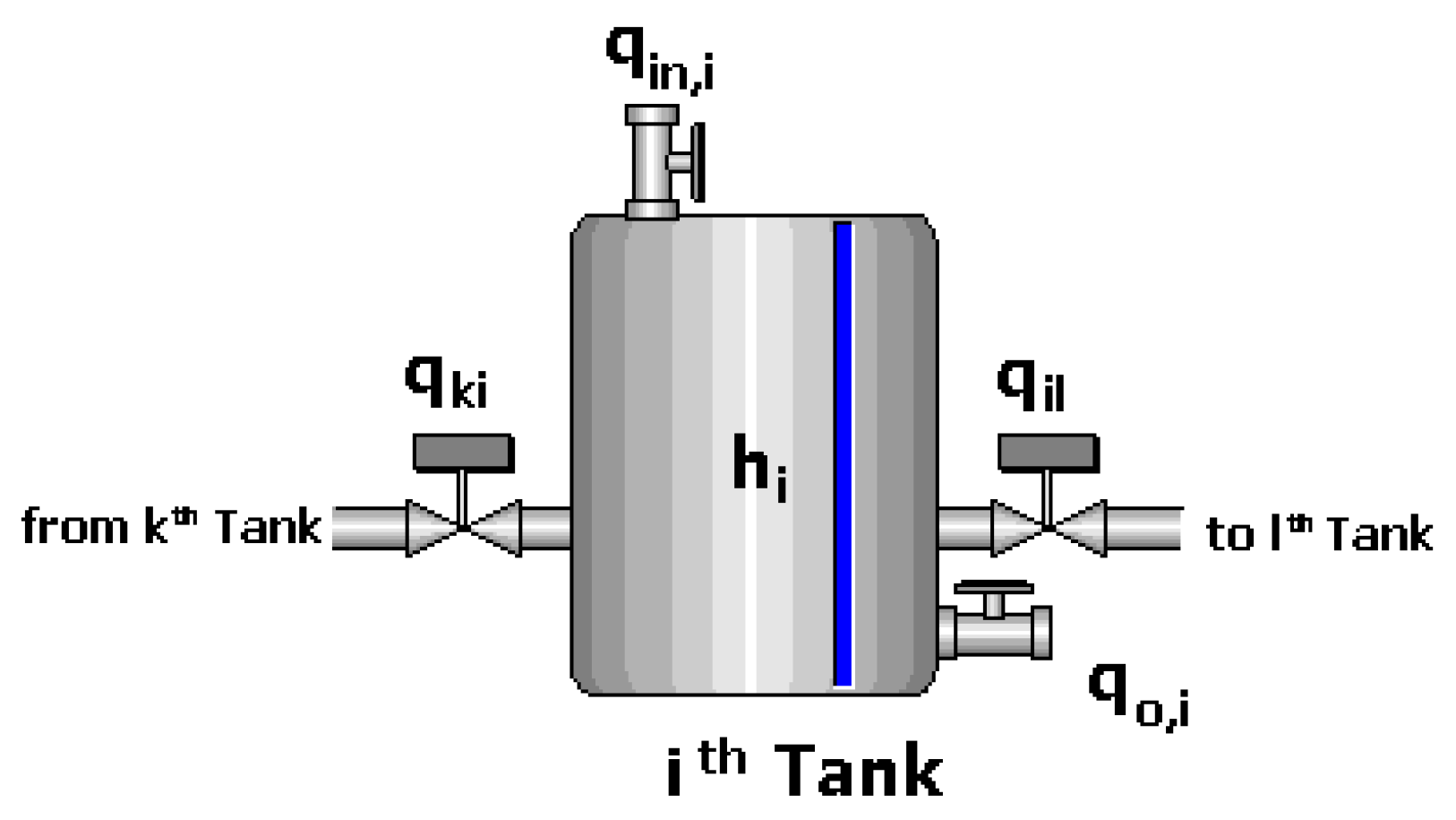
To model the fluid flow rate and pressure in a system of interconnected reservoirs or tanks, one considers the following variables: (1) fluid height in the reservoir/tank h; (2) fluid resistance R, defined as the opposition to the fluid flow in the pipes, i.e., a restriction/valve on the pipe or a load/drain valve; and (3) the coefficient of flow storage in the reservoir (capacitance of the fluid) C, which depends on the area of the reservoir and the density of the fluid [19] (see Figure 1).

Figure 1. Summary of variables in the $i^{th}$ tank.

For now, system uncertainties and external disturbances are not considered for modeling. According to the principle of conservation of material [19], in the $i^{th}$ tank/reservoir, the relationship between fluid level $h_i$ and flow rate $q_i$ is

$$C_i{\displaystyle \frac{d{h}_i}{dt}}=q_i$$

(1)

Further, the total flow rate, i.e., the summation of all flow rates related to the i^th tank in an n-tank system, could be written as

$$q_i=q_{in,i}-q_{o,i}-\sum _{j,\{i,j\}\mathrm{interact}}{q}_{ij}$$

(2)

where $q_{in,i}$ and $q_{o,i}$ are the flow rates for the source and drain of the fluid, respectively, and $q_{ij}$ is the exchanged flow rate between the tanks j that interact with i. Also, the flow rate on the drain $q_{o,i}$ could be approximated to the equation that describes the flow rate through a valve of constant $R_{o,i}$:

$$q_{o,i}={\displaystyle \frac{1}{R_{o,i}}}{h}_i.$$

(3)

3. Modeling as First-Order Coupled System

3.1. Modeling Interacting Tank Without Inputs and Outputs

If the tank does not have external input/output, i.e., a source and drain, and is interacting with other tanks, then $q_{in,i}=0$ and $q_{o,i}=0$ in (2). Further, the exchanged flow rate between tank i and j is $q_{ij}={\displaystyle \frac{1}{R_{ij}}}(h_i-h_j)$$\forall i,j>0$, where $R_{ij}$ is the flow resistance in the pipe (or valve) between tank i and j. Consequently, the level of tank i is given by

$${\dot{h}}_i=-{\displaystyle \frac{h_i}{C_i}}\left(\sum _{j,\{i,j\}\mathrm{interact}}{\displaystyle \frac{1}{R_{ij}}}\right)+{\displaystyle \frac{1}{C_i}}\left(\sum _{j,\{i,j\}\mathrm{interact}}{\displaystyle \frac{h_j}{R_{ij}}}\right),$$

(4)

where “$\{i,j\}\mathrm{interact}$” indicates that there is an interaction between tank i and j.

Considering that the reservoirs/tanks are interconnected through pipes and valves, and hence flows $q_{ij}$, one can specify the coupling between the tanks using a directed weighted graph $G=(V,E)$, where $V=\{i,\dots ,n\}$ is the vertex set that represents each tank, and $E=\{(i,j):w_{ij}\}$ is the edge set that represents the interconnecting pipes/valves, with weights given by $w_{ij}={\displaystyle \frac{1}{R_{ij}{C}_i}}$ [20]. Further, the dynamic model of the whole system of interacting tanks is given by

$$\dot{\overrightarrow{h}}=-\mathcal{L}\overrightarrow{h},$$

(5)

where $\overrightarrow{h}={[h_1,\dots ,h_n]}^T$ is the state vector containing the tanks’ heights, and $\mathcal{L}$ is the Laplacian matrix associated with graph G, defined as [21]

$${\mathcal{L}}_{ij}=\begin{array}{c}\hfill \{\begin{array}{cc}-{\displaystyle \frac{1}{C_i{R}_{ij}}}& \mathrm{if}i\ne j,\{i,j\}\in E,\\ -{\displaystyle \sum _{j,\{i,j\}\in E,i\ne j}}{\mathcal{L}}_{ij}& \mathrm{if}i=j\\ 0& \mathrm{if}\{i,j\}\notin E\end{array},\end{array}$$

(6)

for all $i,j=\{1,2,3,\dots ,n\}$. It should be noted that in this case, the Laplacian matrix $\mathcal{L}$ has non-positive off-diagonal elements, and its diagonal elements are equal to the negative sum of its row elements. Therefore, it has a left eigenvector equal to an all-ones vector ($\overrightarrow{1}$) associated with a zero eigenvalue, i.e., $\mathcal{L}\overrightarrow{1}=0\overrightarrow{1}$ [21].

3.2. Modeling Interacting Tank with Inputs and Outputs

Considering that the system has external sources, which forcibly take out or inject fluid through local control valves that allow the tanks to interact or drain the tanks, the dynamic model of the system of interacting tanks is given by

$${\displaystyle {\dot{h}}_i=-\frac{h_i}{C_i}\left(\frac{1}{R_{o,i}}+\sum _{j,\{i,j\}\mathrm{interact}}\frac{1}{R_{ij}}\right)+\frac{1}{C_i}\left(\sum _{j,\{i,j\}\mathrm{interact}}\frac{h_j}{R_{ij}}\right)-\frac{1}{C_i}\left(\sum _{\{i,j\}\mathrm{interact}}{q}_{i,j}\right)+\frac{q_{in,i}}{C_i},}$$

(7)

In general, one can consider a system of interacting tanks with both external inputs/outputs (flow rates) and local input and outputs to have the form

$$\begin{array}{cc}\hfill \dot{\overrightarrow{h}}& =-\mathcal{L}\overrightarrow{h}+E\overrightarrow{q}+B\overrightarrow{u},\hfill \end{array}$$

(8)

where $\mathcal{L}$ is a Laplacian matrix, $\overrightarrow{u}={[q_{in,1},\dots ,q_{in,p}]}^T$ is the external input vector, $\overrightarrow{q}={[q_{i,j},\dots ,q_{p,q}]}^T$ is the local input vector, and the local input matrix is

$${\displaystyle E_{i,m}=\begin{array}{c}\hfill \{\begin{array}{cc}\frac{1}{C_i}& \mathrm{if}\mathrm{there}\mathrm{is}\mathrm{control}\mathrm{valve}m\mathrm{between}\mathrm{tanks}\mathrm{i}\mathrm{and}\mathrm{j}\\ -\frac{1}{C_j}& \mathrm{if}\mathrm{there}\mathrm{is}\mathrm{control}\mathrm{valve}m\mathrm{between}\mathrm{tanks}\mathrm{j}\mathrm{and}\mathrm{i}\\ 0& \mathrm{otherwise}\end{array},\end{array}}$$

for all $m=1,\dots ,M$ and $i=1,\dots ,n$, where M and n are the numbers of control valves and tanks, respectively. And the input matrix is

$$B_{i,m}=\begin{array}{c}\hfill \{\begin{array}{cc}{\displaystyle \frac{1}{C_i}}& \mathrm{if}\mathrm{there}\mathrm{is}\mathrm{an}\mathrm{external}\mathrm{input}m\mathrm{to}\mathrm{the}\mathrm{tank}i\\ 0& \mathrm{otherwise}\end{array},\end{array}$$

for all $i=1,\dots ,n$ and $m=1,\dots ,p$, where p is the number of external inputs. Further, $\mathcal{L}$ in (8) is the Laplacian matrix of the system’s graph. In this case, the graph associated with the system can include self-edges; that is,

$${\mathcal{L}}_{ij}=\begin{array}{c}\hfill \{\begin{array}{cc}-{\displaystyle \frac{1}{C_i{R}_{ij}}}& \mathrm{if}i\ne j,\{i,j\}\in E,\\ {\displaystyle \frac{1}{C_i{R}_{o,i}}}-{\displaystyle \sum _{j,\{i,j\}\in E,i\ne j}}{\mathcal{L}}_{ij}& \mathrm{if}i=j\\ 0& \mathrm{if}\{i,j\}\notin E\end{array},\end{array}$$

(9)

for all $i,j=\{1,2,3,\dots ,n\}$, where ${\displaystyle \frac{1}{C_i{R}_{o,i}}}$ is a self-edge in the graph G, caused by the drain in a tank i. It should be noted that in this case, the Laplacian matrix $\mathcal{L}$ has non-positive off-diagonal elements, and its diagonal elements are equal to the negative sum of its row elements plus the weight of a self-edge, i.e., it is non-negative. In this case, the matrix $-\mathcal{L}$ is a Metzler matrix, which is commonly found in positive linear dynamical systems [22,23].

3.3. Interconnected Characteristics of the Coupled Model

One of the advantages of representing these systems as a MAS is that Equation (5) works for any interconnection among the tanks. Further, applying the same tools used in networked control systems and MAS [24], one can obtain the following result.

A system of interconnected tanks without inputs and outputs modeled as (4) or (5) reaches consensus if and only if the graph G associated with it is connected, i.e., there is a path between any two vertices in the graph. Further, the consensus height of fluid is $h_i={\sum }_i{w}_i{h}_i\left(0\right)$$\forall i=1,\dots ,n$ (weighted average of the initial tanks’ levels), where $h_i\left(0\right)$ is the initial height of tank i, and $w_i$ is the $i^{th}$ entry of the left eigenvector associated with the eigenvalue ${\lambda }_1=0$ of the Laplacian matrix $\mathcal{L}$ [25]. Moreover, if all the tanks have the same capacitance ($C_i=C\forall i=1,\dots ,n$), then the tanks’ heights converge to ${\displaystyle \frac{1}{n}}{\sum }_i{h}_i\left(0\right)$.

When considering the dynamics with local inputs/outputs $q_{ij}$ (8), the graph representing the coupling may not be connected. However, the local input $q_{ij}$ can locally control the tank level and also connect all the tanks in the systems (through the control valves available in the infrastructure). In this case, the exchange flow rate is $q_{ij}=-{\displaystyle \frac{1}{R_{p_{i,j}}}}\left(h_i-h_j\right)$, where $R_{p_{i,j}}$ is the flow resistance through the valve between tanks i and j, which can be considered static gain in a simple control algorithm. Further, the values of ${\displaystyle \frac{1}{R_{p_{i,j}}}}\ne 0$ generate new edges in the graph G. From the control and graph theory perspective, these new edges must connect the graph, in order to achieve a consensus in the system. Therefore, Equation (8) of the system becomes

$$\dot{\overrightarrow{h}}=-\tilde{\mathcal{L}}\overrightarrow{h}+B\overrightarrow{u},$$

(10)

where $\tilde{\mathcal{L}}$ is the Laplacian matrix of the new graph, and hence has all the properties of any Laplacian matrix.

Moreover, if the tanks have drains, then all the eigenvalues, ${\gamma }_i$, of the Laplacian $\tilde{\mathcal{L}}$ have negative real parts. Hence, the natural response, i.e., $\overrightarrow{u}=\overrightarrow{0}$, of the dynamics in (10) is $\overrightarrow{h}\left(t\right)={\sum }_{i=1}^n{e}^{{\gamma }_{i}t}{v}_i{w}_i^T\overrightarrow{h}\left(0\right)$, whose steady-state value is zero, that is, the dynamics converge to ${lim}_{t\to \infty }{h}_i\left(t\right)=0\forall i=1,\dots ,n$.

4. Modeling as Second-Order Coupled System

4.1. Model Development

In order to define the total flow rate $q_i$ as a state variable, expression (2) is derived:

$${\dot{q}}_i={\dot{q}}_{in,i}-{\displaystyle \frac{1}{R_{oi}}}{\dot{h}}_i-\sum _{j,\{i,j\}\mathrm{interact}}{\dot{q}}_{ij}.$$

(11)

Moreover, using the analysis of the pressure difference at the ends of the pipes that interconnect tanks i and j [19], it is possible to describe the derivative of the flow rate $q_{ij}$ through that pipe as a general expression for the interconnection between tanks i and j: ${\dot{q}}_{ij}=a_{ij}{\displaystyle \frac{\rho }{L_{ij}}}g\left(h_i-h_j\right)$, where $a_{ij}$ and $L_{ij}$ are the cross-section and the length of the pipe between tanks i and j, $\rho$ is the liquid density, g is the gravity constant, and $h_i$ is the fluid height/level in tank i. Therefore, the total derivative of the flow rate exchanged by tank i to the rest of the system can be expressed through the expression

$$\sum _{j,\{i,j\}\mathrm{interact}}{\dot{q}}_{ij}=\rho g\sum _{j,\{i,j\}\mathrm{interact}}{\displaystyle \frac{a_{pij}}{L_{ij}}}\left(h_i-h_j\right),$$

(12)

Furthermore, in taking into account (1) and (3), (11) becomes

$${\dot{q}}_i=-{\displaystyle \frac{1}{R_{o,i}}}{\displaystyle \frac{1}{C_i}}{q}_i-\rho g\sum _{j,\{i,j\}\mathrm{interact}}{\displaystyle \frac{a_{pij}}{L_{ij}}}\left(h_i-h_j\right)+{\dot{q}}_{in,i},$$

(13)

As in Section 3, a weighted graph $G=(V,E)$ represents the coupling between the tanks, where $V=\{i,\dots ,n\}$ is the vertex set that represents each tank, and $E=\{(i,j):w_{ij}\}$ is the edge set that represents the interconnecting pipes, with weights given by $w_{ij}=w_{ji}={\displaystyle \frac{a_{pij}}{L_{ij}}}$. Therefore, the dynamics of the system of interacting tanks can be expressed by a second-order model as

$$\begin{array}{cc}\hfill \left[\begin{array}{c}\dot{\overrightarrow{h}}\\ \dot{\overrightarrow{q}}\end{array}\right]& =\left[\begin{array}{cc}{\mathsf{0}}_{n,n}& \tilde{C}\\ -\rho g{\mathcal{L}}_K& -\tilde{C}{\tilde{R}}_o\end{array}\right]\left[\begin{array}{c}\overrightarrow{h}\\ \overrightarrow{q}\end{array}\right]+\left[\begin{array}{c}{\mathsf{0}}_{n,n}\\ {\mathsf{I}}_{n,n}\end{array}\right]\overrightarrow{u}\hfill \end{array}$$

(14)

where ${\mathsf{0}}_{n,n}$ and ${\mathsf{I}}_{n,n}$ are a zero matrix and the identity matrix, respectively, $\tilde{C}=\mathrm{diag}(C_1^{-1},\dots ,$$C_n^{-1})$ is the matrix whose diagonal corresponds to the inverse of each coefficient of flow storage in every reservoir, ${\tilde{R}}_o=\mathrm{diag}(R_{o,1}^{-1},\dots ,R_{o,n}^{-1})$ is the matrix whose diagonal corresponds to the inverse of the fluid resistances of every reservoir, $\overrightarrow{u}={\left[{\dot{q}}_{in,1},\dots ,{\dot{q}}_{in,n}\right]}^T$, and ${\mathcal{L}}_K$ is the Laplacian matrix

$${\mathcal{L}}_{K_{ij}}=\begin{array}{c}\hfill \{\begin{array}{cc}-{\displaystyle \frac{a_{pij}}{L_{ij}}}& \mathrm{if}i\ne j,\{i,j\}\in E,\\ -{\displaystyle \sum _{j,\{i,j\}\in E,i\ne j}}{\mathcal{L}}_{K_{ij}}& \mathrm{if}i=j\\ 0& \mathrm{if}\{i,j\}\notin E\end{array},\end{array}$$

(15)

for all $i,j=\{1,2,3,\dots ,n\}$.

4.2. Interconnected Characteristics in Tank System Behavior

The state matrix of the dynamics in (14) has the following characteristic equation:

$$\left|{\lambda }^2+\lambda \tilde{C}{\tilde{R}}_o+\rho g{\mathcal{L}}_K\tilde{C}\right|=0,$$

(16)

where $\lambda$ denotes the eigenvalues of the state matrix. Therefore, the eigenvalues $\lambda$ must satisfy the equation ${\lambda }^2+\lambda {\displaystyle \frac{1}{C_i{R}_{o,i}}}+\rho g{\displaystyle \frac{1}{C_i}}{\gamma }_i=0$, where ${\gamma }_i$ is an eigenvalue of ${\mathcal{L}}_K$. Also, given that n eigenvalues of the Laplacian matrix ${\mathcal{L}}_K$ are $0={\gamma }_1\le {\gamma }_2\le \dots \le {\gamma }_n$ [21], the state matrix has at least two real eigenvalues: ${\lambda }_1=0$ and ${\lambda }_2=-{\displaystyle \frac{1}{C{R}_o}}$. Further, the remaining $2n-2$ eigenvalues have negative real parts.

Additionally, if G is connected, then the dominant mode of the dynamics in (14) is $e^{0t}$, of which its response is maintained over time while the effect of the other modes disappears as $t\to \infty$ since the associated eigenvalues have a negative real part. In this regard, we can analyze the behavior of this mode as time grows and whhile considering ${\dot{q}}_{ii}=0$, i.e., the natural response.

The natural response of (14) is given by

$$\left[\begin{array}{c}\overrightarrow{h}\left(t\right)\\ \overrightarrow{q}\left(t\right)\end{array}\right]=\sum _{i=1}^{2n}\left(e^{{\lambda }_{i}t}{v}_i{w}_i^T\right)\left[\begin{array}{c}\overrightarrow{h}\left(0\right)\\ \overrightarrow{q}\left(0\right)\end{array}\right],$$

(17)

where $v_i$ and $w_i^T$ are the right and left eigenvectors associated with the eigenvalue ${\lambda }_i$. Since the eigenvalues ${\lambda }_i\forall i=2,\dots ,2n$ have a negative real part and ${\lambda }_1=0$, the steady state natural response of the system is

$$\begin{array}{c}\hfill \underset{t\to \infty }{lim}\left[\begin{array}{c}\overrightarrow{h}\left(t\right)\\ \overrightarrow{q}\left(t\right)\end{array}\right]=v_1{w}_1^T\left[\begin{array}{c}\overrightarrow{h}\left(0\right)\\ \overrightarrow{q}\left(0\right)\end{array}\right],\end{array}$$

(18)

where $v_1^T=\left[\begin{array}{cc}{\overrightarrow{1}}^T& {\overrightarrow{0}}^T\end{array}\right]$ and $w_i^T={\displaystyle \frac{1}{n}}\left[\begin{array}{cc}{\overrightarrow{1}}^T& {\tilde{R}}_o^{-1}{\overrightarrow{1}}^T\end{array}\right]$ are the right and left eigenvectors associated with the eigenvalue ${\lambda }_1=0$. Therefore, both the fluid height and the flow rate converge to

$$\begin{array}{cc}\hfill \underset{t\to \infty }{lim}{h}_i\left(t\right)& ={\displaystyle \frac{1}{n}}\sum _{i=1}^n{h}_i\left(0\right)+{\displaystyle \frac{1}{n}}\sum _{i=1}^n{R}_{o,i}{q}_i\left(0\right)\hfill \\ \hfill \underset{t\to \infty }{lim}{q}_i\left(t\right)& =0\hfill \end{array}$$

(19)

Moreover, if the initial flow rate is zero, the height in each tank converges to ${\displaystyle \frac{1}{n}}{\sum }_{i=1}^n{h}_i\left(0\right)$, which is the same as in the first-order model.

5. Illustrative Examples

First, let us model the system of three tanks shown in Figure 2 (left) using first-order dynamics.

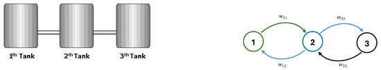
Figure 2. System of three interacting tanks without inputs/outputs (left) and its associated graph (right).

The graph associated with this system has three vertices and edges, as shown in Figure 2 (right). Then, the directions and the weights of the edges depend on the direction of the fluid flow, capacitance of each tank, and resistance of the pipes. For instance, the flows $q_{12}=-q_{21}={\displaystyle \frac{1}{R_{12}}}(h_1-h_2)$ affect the dynamics of tank 1 and 2 and are represented as the directions and weights of the edges between vertices 1 and 2. Therefore, the state matrix of the model (5) is given by

$$\mathcal{L}={\displaystyle \left[\begin{array}{ccc}\frac{1}{R_{12}{C}_1}& -\frac{1}{R_{12}{C}_1}& 0\\ -\frac{1}{R_{12}{C}_2}& (\frac{1}{R_{12}{C}_2}+\frac{1}{R_{23}{C}_2})& \frac{1}{R_{23}{C}_2}\\ 0& -\frac{1}{R_{23}{C}_3}& \frac{1}{R_{23}{C}_3}\end{array}\right]},$$

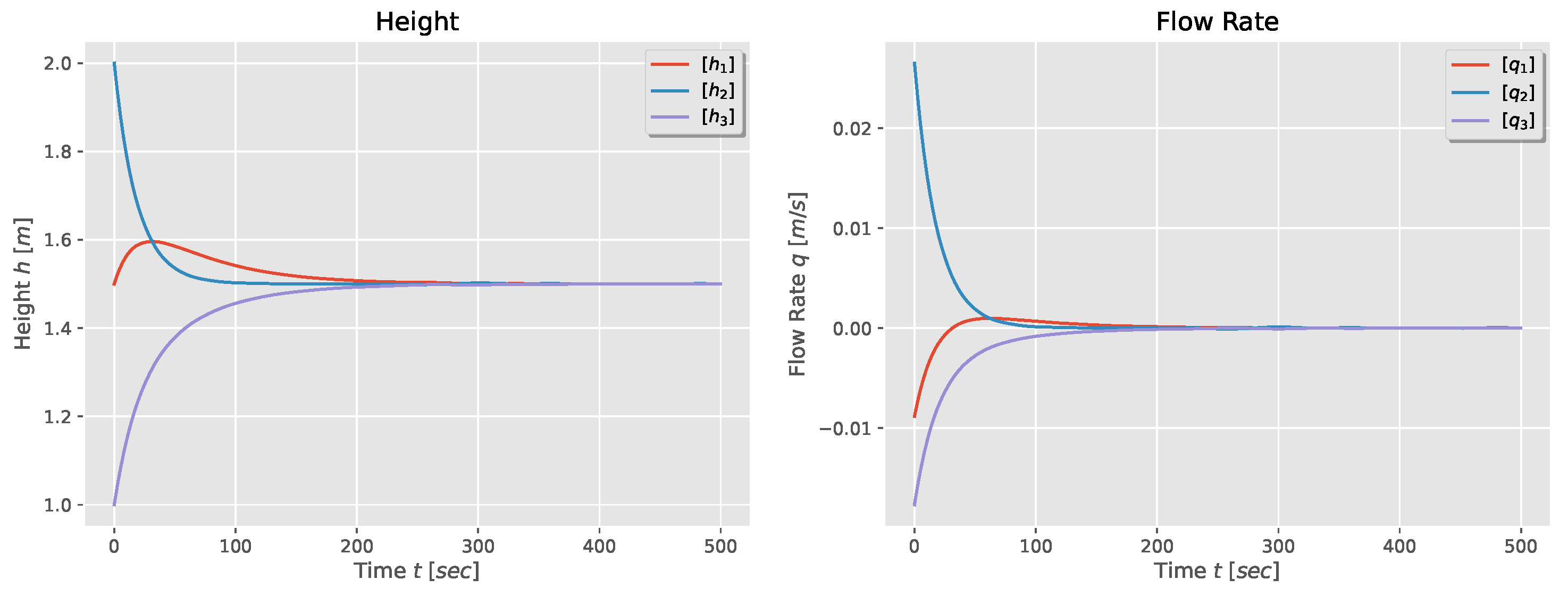
which is the negative of the Laplacian matrix of the graph shown in Figure 2 (right). The natural response of the three-tank dynamics is shown in Figure 3. One observes that the tanks’ height reaches consensus with the weighted average of the initial heights, while the flow rate in each tank becomes zero.

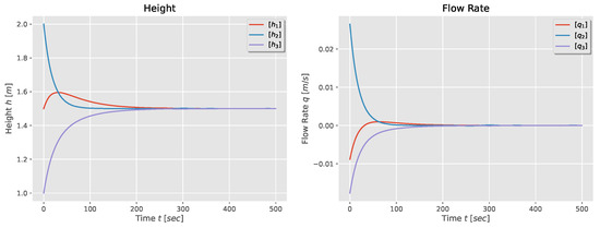
Figure 3. Height and flow rate for a first-order model of a three-tank system.

Meanwhile, using second-order dynamics, (14), where ${\mathcal{L}}_K$ is

$${\mathcal{L}}_K={\displaystyle \left[\begin{array}{ccc}\frac{a_{p12}}{L_{12}}& -\frac{a_{p12}}{L_{12}}& 0\\ -\frac{a_{p12}}{L_{12}}& (\frac{a_{p12}}{L_{12}}+\frac{a_{p23}}{L_{23}})& -\frac{a_{p23}}{L_{23}}\\ 0& -\frac{a_{p23}}{L_{23}}& \frac{a_{p23}}{L_{23}}\end{array}\right]}$$

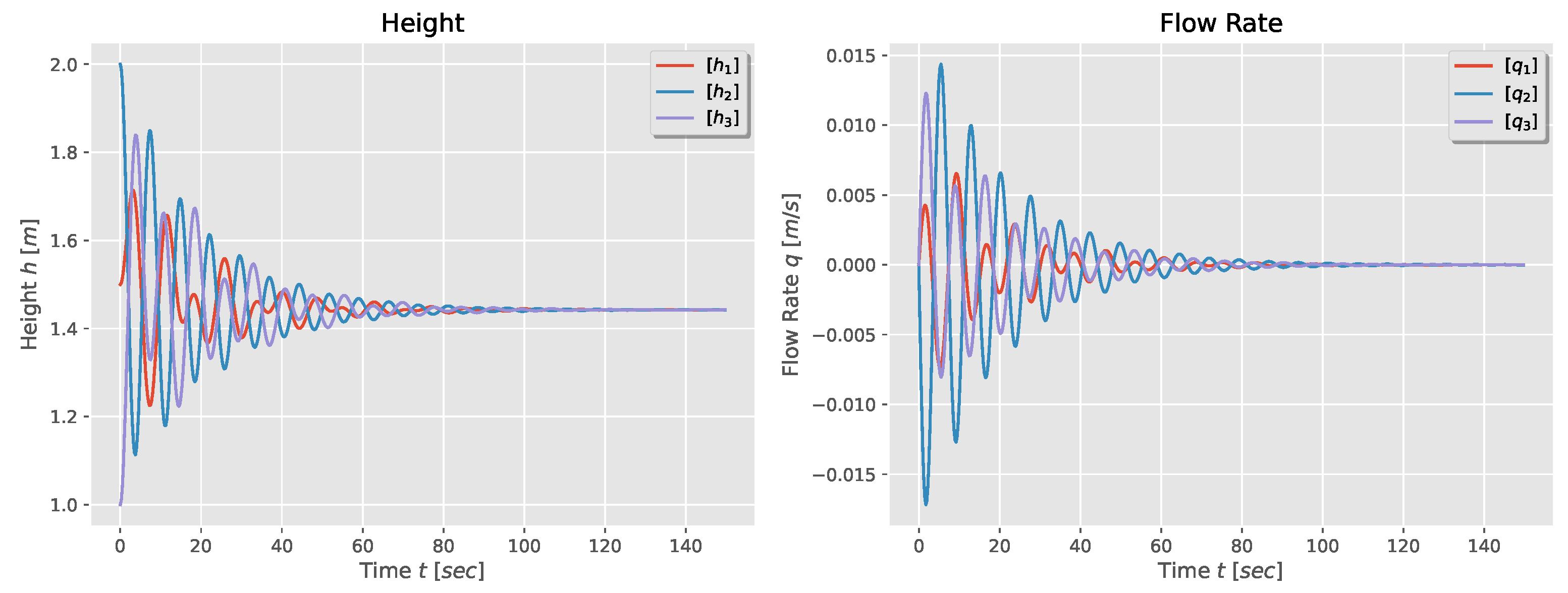
the natural response of the system is faster than its first-order counterpart, and it has an oscillatory behavior due to the presence of complex modes in system (14), as shown in Figure 4. It is observed that the tanks’ height reaches consensus with a value that depends of the initial heights, and the flow rate in each tank becomes zero, which means that exchanged flow rate through the pipes between tanks will be zero too.

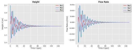
Figure 4. Height and flow rate for a second-order model of a three-tank system.

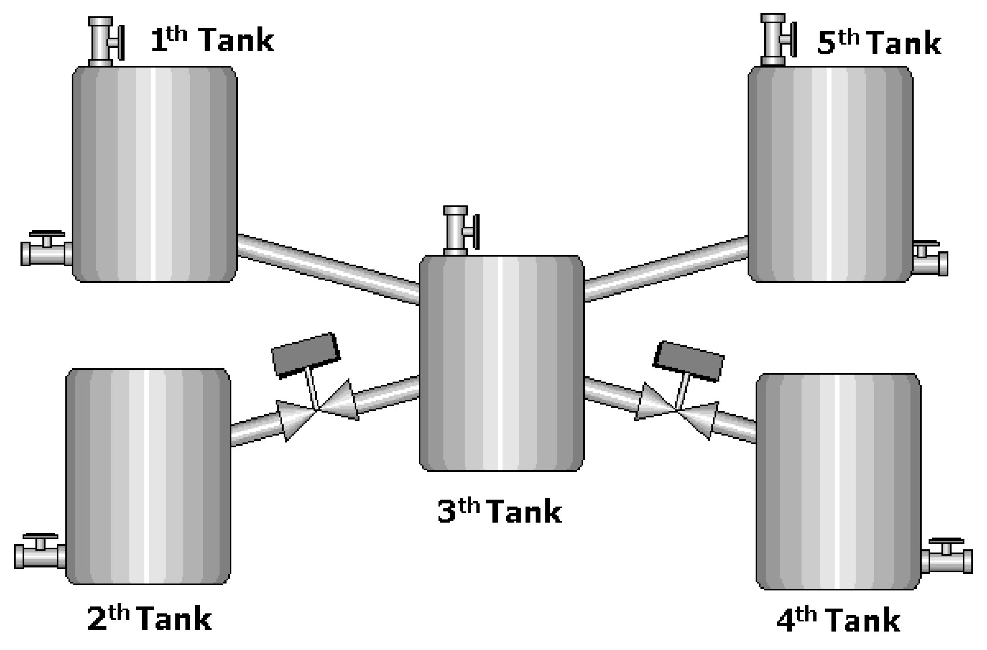
Now, consider a five-tank system as shown in Figure 5, where there are control valves between tanks 2 and 3 and between 3 and 4, i.e., the dynamics corresponding to tanks 2, 3, and 4 have local inputs/outputs. Further, tanks 1, 3, and 5 have external inputs and tanks $1,2,4$, and 5 have an output flow.

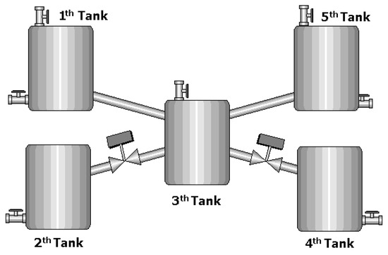
Figure 5. System of five interacting tanks.

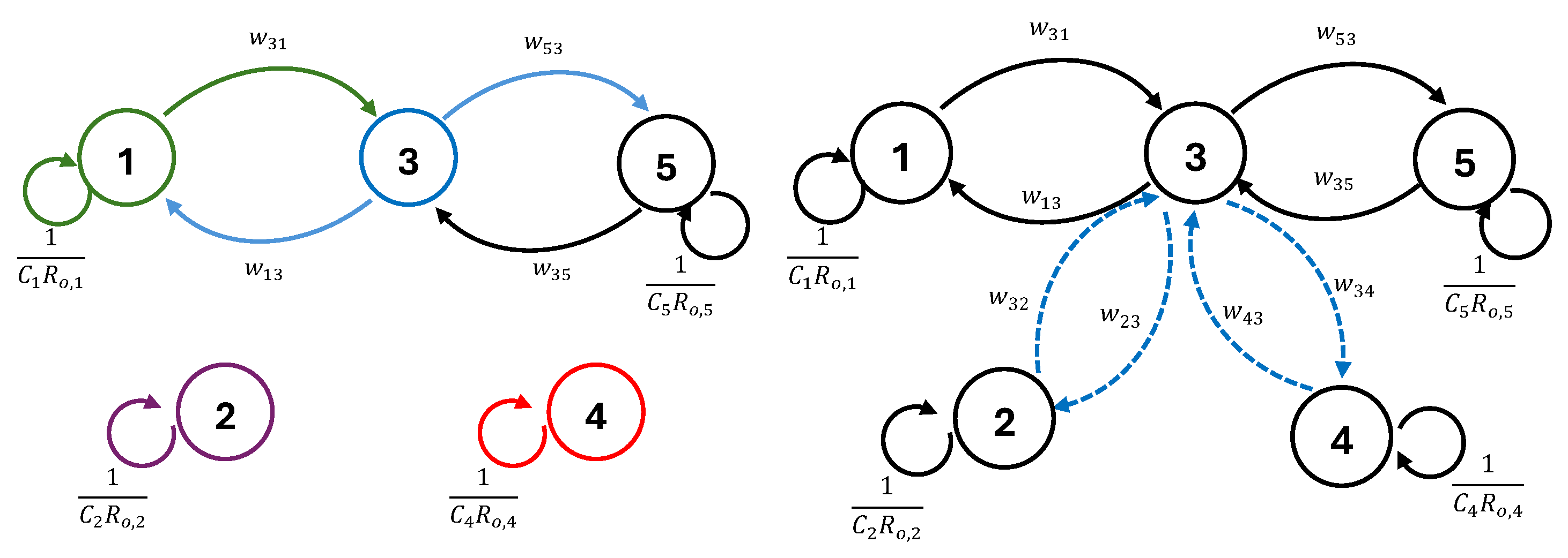
The graph associated with this system is shown in Figure 6 (right), which includes self-edges in all the vertices. Moreover, the graph is not connected since vertices 2 and 4 are isolated; however, these vertices, together with vertex 3, have local inputs. The system dynamics are

$${\displaystyle \begin{array}{ccc}\hfill \dot{\overrightarrow{h}}& =-\mathcal{L}\overrightarrow{h}\hfill & \hfill +\left[\begin{array}{cc}0& 0\\ \frac{1}{C_2}& 0\\ -\frac{1}{C_3}& -\frac{1}{C_3}\\ 0& \frac{1}{C_4}\\ 0& 0\end{array}\right]\left[\begin{array}{c}{q}_{23}\\ q_{43}\end{array}\right]+\left[\begin{array}{ccc}\frac{1}{C_1}& 0& 0\\ 0& 0& 0\\ 0& \frac{1}{C_3}& 0\\ 0& 0& 0\\ 0& 0& \frac{1}{C_5}\end{array}\right]\left[\begin{array}{c}{q}_{in,1}\\ q_{in,3}\\ q_{in,5}\end{array}\right]\end{array}}$$

(20)

where $\overrightarrow{h}={\left[\begin{array}{ccc}{h}_1& \cdots & h_5\end{array}\right]}^T$ and $\mathcal{L}={\displaystyle \left[\begin{array}{ccccc}\frac{1}{C_1}\left(\frac{1}{R_{o1}}+\frac{1}{R_{13}}\right)& 0& -\frac{1}{C_1}\frac{1}{R_{13}}& 0& 0\\ 0& \frac{1}{C_2}\frac{1}{R_{o,2}}& 0& 0& 0\\ -\frac{1}{C_3}\frac{1}{R_{13}}& 0& \frac{1}{C_3}\left(\frac{1}{R_{35}}+\frac{1}{R_{13}}\right)& 0& -\frac{1}{C_3}\frac{1}{R_{35}}\\ 0& 0& 0& \frac{1}{C_4}\frac{1}{R_{o,4}}& 0\\ 0& 0& -\frac{1}{C_5}\frac{1}{R_{35}}& 0& \frac{1}{C_5}\left(\frac{1}{R_{o,5}}+\frac{1}{R_{35}}\right)\end{array}\right]}$.

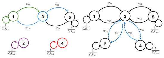
Figure 6. Graphs of the system with five interconnected tanks with closed control valves (left) and open control valves (right) between tanks 2, 3, and 4.

Once, the valves between tanks 2 and 3 and tanks 3 and 4 are open, the dynamics of the system are given by (10), as shown in Figure 6 (left), with Laplacian matrix

$\tilde{\mathcal{L}}={\displaystyle \left[\begin{array}{ccccc}\frac{1}{C_1}\left(\frac{1}{R_{o1}}+\frac{1}{R_{13}}\right)& 0& -\frac{1}{C_1}\frac{1}{R_{13}}& 0& 0\\ 0& \frac{1}{C_2}\left(\frac{1}{R_{o,2}}+\frac{1}{R_{p2,3}}\right)& -\frac{1}{C_2}\frac{1}{R_{p2,3}}& 0& 0\\ -\frac{1}{C_3}\frac{1}{R_{13}}& -\frac{1}{C_3}\frac{1}{R_{p2,3}}& \frac{1}{C_3}\left(\frac{1}{R_{35}}+\frac{1}{R_{13}}+\frac{1}{R_{p2,3}}+\frac{1}{R_{p3,4}}\right)& -\frac{1}{C_3}\frac{1}{R_{p3,4}}& -\frac{1}{C_3}\frac{1}{R_{35}}\\ 0& 0& -\frac{1}{R_{p3,4}}& \frac{1}{C_4}\left(\frac{1}{R_{o,4}}+\frac{1}{R_{p3,4}}\right)& 0\\ 0& 0& -\frac{1}{C_5}\frac{1}{R_{35}}& 0& \frac{1}{C_5}\left(\frac{1}{R_{o,5}}+\frac{1}{R_{35}}\right)\end{array}\right]}$

For the second-order model, the dynamics of the five tanks given by (14) uses

${\mathcal{L}}_K={\displaystyle \left[\begin{array}{ccccc}\frac{a_{p13}}{L_{13}}& 0& -\frac{a_{p13}}{L_{13}}& 0& 0\\ 0& \frac{a_{p23}}{L_{23}}& -\frac{a_{p23}}{L_{23}}& 0& 0\\ -\frac{a_{p13}}{L_{13}}& -\frac{a_{p23}}{L_{23}}& \left(\frac{a_{p13}}{L_{13}}+\frac{a_{p23}}{L_{23}}+\frac{a_{p34}}{L_{34}}+\frac{a_{p35}}{L_{35}}\right)& -\frac{a_{p34}}{L_{34}}& -\frac{a_{p35}}{L_{35}}\\ 0& 0& -\frac{a_{p34}}{L_{34}}& \frac{a_{p34}}{L_{34}}& 0\\ 0& 0& -\frac{a_{p35}}{L_{35}}& 0& \frac{a_{p34}}{L_{34}}\end{array}\right]}$

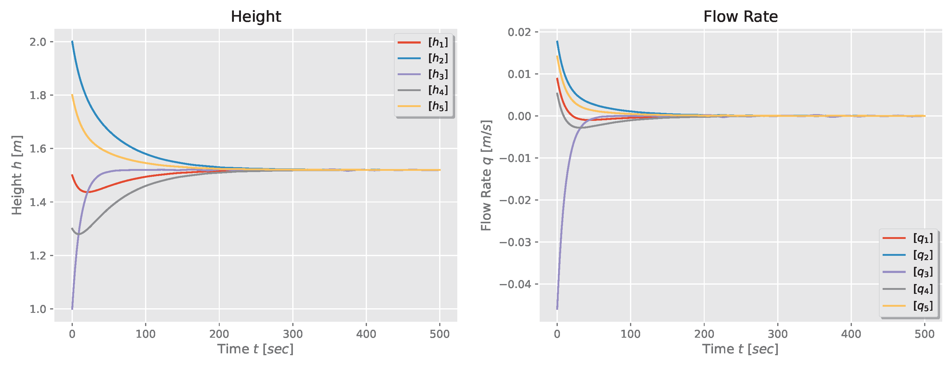
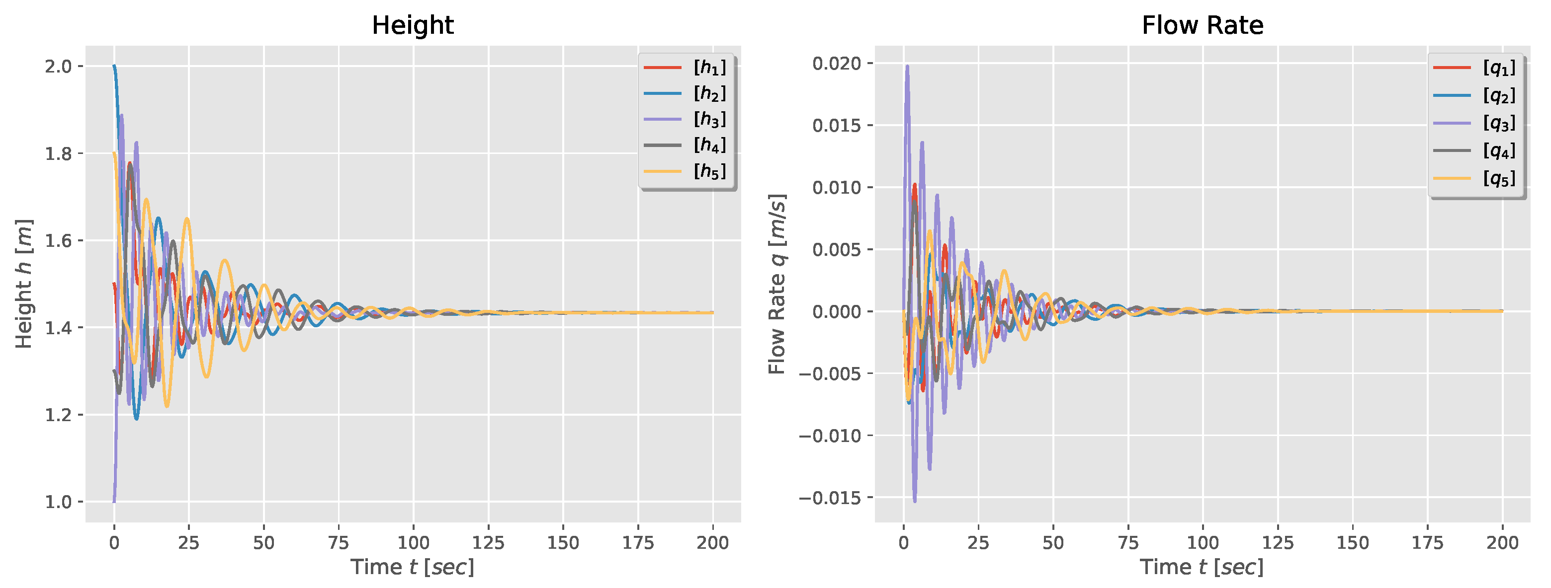
Finally, the natural response of the five-tank system for a first-order and second-order model are shown in Figure 7 and Figure 8. Again, one observes that the tanks’ height and flow rate reach consensus: the heights converge to the weighted average of the initial heights, while the flow rates converge to zero.

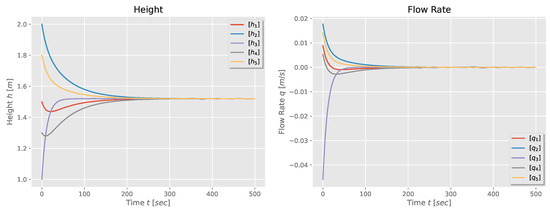
Figure 7. Height and flow rate for a first-order model of a five-tank system in star configuration.

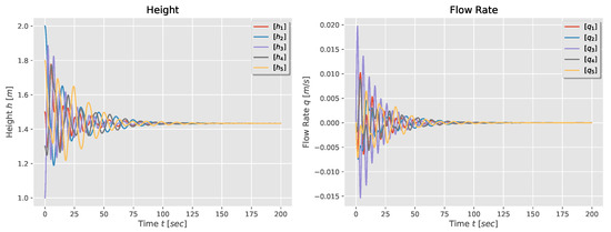
Figure 8. Height and flow rate for a second-order model of a five-tank system in star configuration.

6. Conclusions

The interacting tank model described in this study was modeled as a coupled/interconnected system that can employ any configuration for the interconnection between the tanks and is scalable to n agents. Furthermore, it employs analytical techniques to support the modeling, including graph and spectral graph theory, and control theory to analyze and characterize the behavior of individual agents as well as the system as a whole. Using this MAS approach, the system is viewed as a collection of independent agents cooperating to achieve a shared goal, namely the convergence of heights, which acts as a stepping stone to apply control algorithms designed for cyber-physical systems to this type of system.

References

- Uhrmacher, A.M.; Weyns, D. Multi-Agent Systems: Simulation and Applications; CRC Press: Boca Raton, FL, USA, 2009. [Google Scholar]
- Busoniu, L.; Babuska, R.; De Schutter, B. A comprehensive survey of multiagent reinforcement learning. IEEE Trans. Syst. Man Cybern. Part C (Appl. Rev.) 2008, 38, 156–172. [Google Scholar] [CrossRef]
- Rizk, Y.; Awad, M.; Tunstel, E.W. Decision Making in Multiagent Systems: A Survey. IEEE Trans. Cogn. Dev. Syst. 2018, 10, 514–529. [Google Scholar] [CrossRef]
- Oprea, M. Applications of multi-agent systems. In Information Technology; Springer: Cham, Switzerland, 2004; pp. 239–270. [Google Scholar]
- Sycara, K.P. Multiagent systems. AI Mag. 1998, 19, 79. [Google Scholar]
- Wang, B.; Wang, J.; Zhang, B.; Li, X. Global Cooperative Control Framework for Multiagent Systems Subject to Actuator Saturation With Industrial Applications. IEEE Trans. Syst. Man Cybern. Syst. 2017, 47, 1270–1283. [Google Scholar] [CrossRef]
- Wang, B.; Wang, J.; Zhang, B.; Chen, W.; Zhang, Z. Leader–Follower Consensus of Multivehicle Wirelessly Networked Uncertain Systems Subject to Nonlinear Dynamics and Actuator Fault. IEEE Trans. Autom. Sci. Eng. 2018, 15, 492–505. [Google Scholar] [CrossRef]
- Nunavath, V.; Prinz, A. Visualization of exchanged information with dynamic networks: A case study of fire emergency search and rescue operation. In Proceedings of the 2017 IEEE 7th International Advance Computing Conference (IACC), Hyderabad, India, 5–7 January 2017; pp. 281–286. [Google Scholar]
- Merabet, G.H.; Essaaidi, M.; Talei, H.; Abid, M.R.; Khalil, N.; Madkour, M.; Benhaddou, D. Applications of multi-agent systems in smart grids: A survey. In Proceedings of the 2014 International Conference on Multimedia Computing and Systems (ICMCS), Marrakech, Morocco, 14–16 April 2014; pp. 1088–1094. [Google Scholar]
- Maldonado, D.; Cepeda, J.; Gamboa, S.; Torres, J.A.; Cruz, P.J. Optimum frequency response with decentralized drivers in power system. IET Gener. Transm. Distrib. 2023, 17, 1985–1998. [Google Scholar] [CrossRef]
- Kuo, M.T.; Lu, S.D. Design and implementation of real-time intelligent control and structure based on multi-agent systems in microgrids. Energies 2013, 6, 6045–6059. [Google Scholar] [CrossRef]
- Leite, J.; Omicini, A.; Sterling, L.; Torroni, P. Declarative Agent Languages and Technologies: First International Workshop, DALT 2003, Melbourne, Australia, July 15, 2003, Revised Selected and Invited Papers; Springer: Cham, Switzerland, 2004; Volume 2990. [Google Scholar]
- Gatzke, E.P.; Meadows, E.S.; Wang, C.; Doyle Iii, F.J. Model based control of a four-tank system. Comput. Chem. Eng. 2000, 24, 1503–1509. [Google Scholar] [CrossRef]
- Naik, R.B.; Kanagalakshmi, S. Mathematical modelling and controller design for interacting hybrid two tank system (IHTTS). In Proceedings of the 2020 Fourth International Conference on Inventive Systems and Control (ICISC), Coimbatore, India, 8–10 January 2020; pp. 297–303. [Google Scholar]
- Balakrishnaa, A.; Arun, N. Liquid level control of interacting coupled spherical tank system using PI and Fuzzy Pi Controller. In Proceedings of the 2022 3rd International Conference for Emerging Technology (INCET), Belgaum, India, 27–29 May 2022; pp. 1–5. [Google Scholar]
- Hajebi, S.; Barrett, S.; Clarke, A.; Clarke, S. Multi-agent simulation to support water distribution network partitioning. In Proceedings of the 27th European Simulation and Modelling Conference, Alesund, Norway, 27–30 May 2013. [Google Scholar]
- Kordestani, M.; Safavi, A.A.; Sharafi, N.; Saif, M. Novel multiagent model-predictive control performance indices for monitoring of a large-scale distributed water system. IEEE Syst. J. 2016, 12, 1286–1294. [Google Scholar] [CrossRef]
- Dötsch, F.; Denzinger, J.; Kasinger, H.; Bauer, B. Decentralized real-time control of water distribution networks using self-organizing multi-agent systems. In Proceedings of the 2010 Fourth IEEE International Conference on Self-Adaptive and Self-Organizing Systems, Budapest, Hungary, 27 September–1 October 2010; pp. 223–232. [Google Scholar]
- Wellstead, P.E. Introduction to Physical System Modelling; Academic Press: London, UK, 2005; Volume 4. [Google Scholar]
- Diestel, R. Graph Theory; (print edition); Springer: New York, NY, USA, 2024. [Google Scholar]
- Chung, F.R. Spectral Graph Theory; American Mathematical Soc.: Providence, RI, USA, 1997; Volume 92. [Google Scholar]
- Duan, X.; Jafarpour, S.; Bullo, F. Graph-theoretic stability conditions for Metzler matrices and monotone systems. SIAM J. Control Optim. 2021, 59, 3447–3471. [Google Scholar] [CrossRef]
- Cvetković, A. Stabilizing the Metzler matrices with applications to dynamical systems. Calcolo 2020, 57, 1. [Google Scholar] [CrossRef]
- Oh, K.K.; Park, M.C.; Ahn, H.S. A survey of multi-agent formation control. Automatica 2015, 53, 424–440. [Google Scholar] [CrossRef]
- Pirani, M.; Sundaram, S. Spectral properties of the grounded Laplacian matrix with applications to consensus in the presence of stubborn agents. In Proceedings of the 2014 American Control Conference, Portland, OR, USA, 4–6 June 2014; pp. 2160–2165. [Google Scholar]
Disclaimer/Publisher’s Note: The statements, opinions and data contained in all publications are solely those of the individual author(s) and contributor(s) and not of MDPI and/or the editor(s). MDPI and/or the editor(s) disclaim responsibility for any injury to people or property resulting from any ideas, methods, instructions or products referred to in the content. |
© 2024 by the authors. Licensee MDPI, Basel, Switzerland. This article is an open access article distributed under the terms and conditions of the Creative Commons Attribution (CC BY) license (https://creativecommons.org/licenses/by/4.0/).