An Alternative Method to Measure Glucose and Lactic Acid as Biomarkers of the Postmortem Interval (PMI)

Abstract

Background: In forensic investigations, the postmortem interval (PMI) is still mainly determined using pathological analysis. There have been many scientific efforts to identify alternative methods of PMI determination, which may be applied to future forensic practices. Methods: Considering the ethical implications and the availability of tissue samples for PMI experiments, we used human blood samples stored at three temperatures to mimic different environmental conditions, testing them over a period of 10 days post-sampling. These samples were biochemically tested for specific blood biomarkers, glucose (Glu) and lactic acid (Lac), to determine their potential as PMI biomarkers. Then, a mixed-effect mathematical model was applied to the data related to time- and temperature-dependent concentration changes of both biomarkers followed by additional computer-simulated models to refine the PMI estimates based on each of the biomarker concentration changes. Results: Herein, we present this alternative method of PMI estimation based on the biochemical testing of blood samples that could potentially be collected at a crime scene using biochemical blood biomarkers Glu and Lac, which are mathematically modelled and refined with time- and temperature concentration changes. Conclusions: While there is still much forensic science required to validate any alternative PMI methods, this study shows that there are other cross-disciplinary methods of PMI determination that warrant further exploration.

1. Introduction

The post-mortem interval (PMI), also known as the time since death, is essential information during criminal investigations when a sudden or suspicious death occurs. By determining the PMI, it is possible to narrow down a list of suspects, accept or reject the alibis of people under investigation, and verify witnesses’ statements [1]. For these reasons, an accurate and precise PMI is critical. PMI can be classified into the three physiological stages of immediate, early, and late. The immediate stage, lasting from 30 min to 2 h, involves rapid changes due to a lack of blood circulation and, as a result, the disruption of all biological mechanisms. The early stage, spanning 3 to 72 h after death, is when macroscopic decomposition changes become more recognizable, and most forensic cases are examined during this time [2]. The late stage, starting after three days in an unrefrigerated body exposed to a temperate climate, involves drastic changes such as putrefaction [3] (p. 64). The assessment of PMI in the early stage is made possible through the observation of specific physiological changes over a short time, such as rigor mortis, algor mortis, and livor mortis (body rigidity, heat loss, and skin discoloration, respectively). However, these visible changes are influenced by surrounding environmental factors. The chances of errors occurring increase when physical changes are used to quantify the PMI, as these parameters are quickly affected by external conditions [4]. Hence, there are limitations defining PMI, which often leads to a large postmortem window [5] because the decomposition of human remains involves complex and highly variable processes [6]. To improve the accuracy and precision of the PMI estimate, forensic scientists have tried to identify alternative biochemical tests that can be used as an auxiliary method of PMI assessment [7]. It was hypothesized that the metabolic time-dependent changes occurring in blood immediately after death might produce molecules that are suitable biochemical markers for assessing the PMI [8,9]. Therefore, the collection of blood samples from a deceased body to measure specific PMI biomarkers could potentially be incorporated into future PMI determination in forensic practices.

There are, however, disadvantages to blood sampling at a crime scene that can make samples challenging to analyze. This is mostly due to biochemical changes that are caused by hemolytic and putrefactive events [10]. In addition, like most forensic samples, blood is not always easy to collect in a timely manner and is often only available in a small amount [11]. Furthermore, inter-individual variability [12] and temperature fluctuations [13,14] can significantly affect blood composition, adding complexity to its analysis. For this reason, it is not common to use blood samples to assess PMI during crime investigations [15]. Nonetheless, the identification of reliable PMI biomarkers from blood could lead to more effective forensic blood sampling and testing strategies in forensic laboratories.

Glucose (Glu) and lactic acid (Lac) are two blood biomarkers that are often used to diagnose and monitor metabolic diseases [16]. Those two biomarkers are easily detected and quantified using many commercial assays developed for patient blood samples. In decomposing subjects’ blood samples, they also present recognizable time-dependent patterns, albeit non-linear ones [17]. Thus, there is potential to further explore Glu and Lac as PMI biomarkers to calculate PMI for future forensic practice.

Even so, biochemical tests alone are not a sufficiently a reliable method for assessing PMI and can be significantly improved by incorporating statistical modelling to determine efficacy and precision [18]. Statistical tools and mathematical modelling have become increasingly important in forensic science and forensic medicine. The use of corrective factors to minimize errors [19], non-linear models [20], multiple readings of a given parameter [21], and mixed-effect modelling [22] have been proven to increase the precision and accuracy of PMI estimations.

The main objective of this research was to develop a methodology for biomarker discovery in PMI estimation using blood samples from 20 healthy donors. Blood glucose (Glu) and lactic acid (Lac) were evaluated as potential PMI biomarkers by modelling their kinetics over time in human blood plasma for 10 consecutive days. To account for inter-individual variability, the mixed-effects mathematical model was applied, to improve the precision and accuracy of the PMI estimation.

The data were used to establish a correlation between Glu and Lac biomarker concentrations over time and temperature parameters. The impact of temperature on these biomarkers was modelled using Arrhenius temperature-dependence secondary models to reduce the bias caused by temperature fluctuations. An experimental sampling strategy was designed to optimize PMI assessments, exploring the best combinations of three key factors: (1) consecutive days of sampling, (2) the sampling frequency, and (3) the required number of replicates. A simulated experiment was conducted to estimate PMI using data obtained from the analyzed blood samples. The application of these mathematical models and methodologies provided a robust experimental and modelling approach to enhance the reliability of PMI estimations.

2. Materials and Methods

2.1. Donor Samples

First, 9 mL of whole blood was collected in VACUETTE^® tubes (K3EDTA) from 20 healthy donors within our research institute who had first provided informed ethical consent to the study. The study was approved by the Technological University Dublin ethics committee (ref. number REC-18-118) prior to commencement. The inclusion criteria for donor sampling were as follows: those deemed to be of normal health, within an age range of 20–50 years old, of mixed genders (12 female and18 males), and with no known underlying conditions nor history of medication usage at the time of sampling. After blood collection, the tubes were centrifuged at 500 rpm for 5 min to separate the plasma from the blood cell populations (erythrocytes and leucocytes). The concentrations of two biomarkers, Glu and Lac, was measured using commercial colorimetric tests (detailed below). Then, all samples were stored at three different temperatures as follows: 10 tubes stored at 20 °C, 5 tubes stored at 10 °C, and 5 tubes stored at 30 °C. Every day, for 10 consecutive days, the biomarker tests were repeated, with tubes inverted 5 times before centrifugation at 500 rpm for 5 min before the concentrations of Glu and Lac were measured each day.

2.2. Glucose and Lactic Acid Colorimetric Test

To measure both the concentration of Glu and Lac in plasma from the donor’s blood samples, a colorimetric kit assay was used for each biomarker according to the kit instructions (Audit Diagnostic, Cork Ireland, distributed by Glenbio Co., Antrim, UK). Briefly, to test the concentration of Glu, 1000 µL of reagent 1 was added to 10 µL of plasma in each of the test wells on the 24-well plate. The plate was incubated at 37 °C for 5 min, and the absorbance at 504 nm was measured using a Varioskan™ LUX multimode microplate reader (Thermo Fisher Scientific, Rath Business Park, Hollywoodrath, Dublin, D15 KW24, Ireland). The same protocol was followed to test the concentration of Lac using the specific reagent from the lactic acid test kit. The plate was then incubated at room temperature for 10 min, and the absorbance was measured at 546 nm using a Varioskan™ LUX multimode microplate reader (Thermo Fisher Scientific). This method was repeated for ten consecutive days for each sample stored at the previously mentioned temperatures of 10 °C, 20 °C and 30 °C.

2.3. Population Model for the Kinetics of the Two Markers

A mathematical model describing the behaviour of Glu and Lac over time was built. All Glu and Lac concentration data were analysed using R software version 4.1.1 (R Core Team 2021). The model from Beneke et al. [23] was used to describe the kinetics of Lac. For Glu, we used a model mixing a first-order asymptotic production [24] with a Weibull process [25] to describe the observed release of Glu over longer periods.

All of the Glu and Lac model parameters were estimated using non-linear mixed-effect regression. Each parameter’s variability among individuals was then evaluated by comparing its variance to its mean value. If a parameter’s variance was less than 0.01% of its mean, it was considered fixed for the entire population. Additionally, various combinations of fixed and random parameters were tested using the likelihood ratio test, the Akaike Information Criterion (AIC), and the Bayesian Information Criterion (BIC) to develop the simplest final model [26].

Equations (1) and (2) describe the kinetics of Glu and Lac, respectively:

$$Gl{u}_{ij}~{Glus0}_i·e^{-e^{lke{l}_i}·Da{y}_j}+e^{lm{l}_i·{Da{y}_j}^{S_i}}+{\in }_{ij}$$

(1)

$$La{c}_{ij}~L_{{max}_i}·{\displaystyle \frac{e^{{lk1}_i}}{e^{{lk1}_i}-e^{{lk2}_i}}}·\left(e^{{-e}^{{lk1}_i}·Da{y}_j}-e^{{-e}^{{lk2}_i}·Da{y}_j}\right)+L_{0_i}+{\in }_{ij}$$

(2)

Equations (3) and (4) define the parameters’ random effect structure, where Glus0 is the initial Glu concentration (mmol/L); lkel is the natural logarithm of the apparent first-order rate constant of elimination (day-1); lml is the natural logarithm of the rate constant for haemolysis-based Glu increase; s is the shape parameter for haemolysis-based Glu increase; lk1 is the natural logarithm of the apparent first-order rate constant of production (day-1); lk2 is the natural logarithm of the elimination apparent first-order rate constant (day-1); Lmax is the maximal amount of Lac available (mmol/L); L0 is the initial concentration of Lac (mmol/L); i denotes the parameter for the individual i and j indicates the measurement j inside individual i:

$$\left[\begin{array}{c}\begin{array}{c}{Glus0}_{\mathit{i}}\\ lke{l}_i\\ lm{l}_i\end{array}\\ s_i\end{array}\right]~N\left(\left[\begin{array}{c}\begin{array}{c}\begin{array}{c}\overline{Glus0}\\ \overline{lkel}\end{array}\\ \overline{lml}\end{array}\\ \overline{s}\end{array}\right],\left[\begin{array}{c}\begin{array}{c}\begin{array}{c}{\sigma }_{Glus0}\\ {\sigma }_{lkel}\end{array}\\ {\sigma }_{lml}\end{array}\\ {\sigma }_s\end{array}\right]\mathrm{ }\right)$$

(3)

$$\left[\begin{array}{c}\begin{array}{c}{L}_{{max}_i}\\ {lk1}_i\\ {lk2}_i\end{array}\\ L_{0_i}\end{array}\right]~N\left(\left[\begin{array}{c}\begin{array}{c}\begin{array}{c}\overline{L_{{max}_i}}\\ \overline{lk1}\end{array}\\ \overline{lk2}\end{array}\\ \overline{L_0}\end{array}\right],\left[\begin{array}{c}\begin{array}{c}\begin{array}{c}{\sigma }_{Glus0}\\ {\sigma }_{lkel}\end{array}\\ {\sigma }_{lml}\end{array}\\ {\sigma }_s\end{array}\right]\mathrm{ }\right)$$

(4)

where σ is the standard deviation of normal distributions representing deviation differences between individuals i in all the model parameters. The accent “ ̅ ” denotes the mean of the normal distributions.

Equations (5)–(7) allow for the secondary modelling of the parameters using an Arrhenius temperature dependence with a reference temperature [27]:

$$\overline{lkel}~{lkel}_{T_{ref}}-{\displaystyle \frac{{Ea}_{kel}}{R}}\left({\displaystyle \frac{1}{T}}-{\displaystyle \frac{1}{T_{ref}}}\right)$$

(5)

$$\overline{lml}~{lml}_{T_{ref}}-{\displaystyle \frac{{Ea}_{ml}}{R}}\left({\displaystyle \frac{1}{T}}-{\displaystyle \frac{1}{T_{ref}}}\right)$$

(6)

$$\overline{lk2}~{lk2}_{T_{ref}}-{\displaystyle \frac{{Ea}_{k2}}{R}}\left({\displaystyle \frac{1}{T}}-{\displaystyle \frac{1}{T_{ref}}}\right)$$

(7)

where Ea is the energy of activation (KJ/Mol); R is the universal gas constant 8.303 × 10⁻³ KJ/Mol/K; Temp is the temperature in Kelvin; and Tref is the reference temperature 20 + 273K.

Finally, Equation (8) adds a normal error distribution to model the experimental responses:

$${\in }_{ij}~N\left(0,\left[\begin{array}{c}{\sigma }_{Glu}\\ {\sigma }_{Lac}\end{array}\right] \right)$$

(8)

where ∈ is the experimental precision defined by two independent normal distributions, one for Glu and one for Lac.

2.4. Effect of the Postmortem Sampling Design in the Accuracy and Precision of the PMI Estimate

Once the model was built, we aimed to simulate the effect of a sampling strategy with several consecutive measurements on the accuracy and precision of the estimate of the postmortem interval (PMI). Precision was defined as the standard error of the non-linear regression estimate of the PMI for a specific simulated postmortem sampling design. Meanwhile, bias, used to measure accuracy, was defined as the difference between the estimated PMI’s absolute value and the PMI’s absolute value defined as “true” during the simulation.

To assess the postmortem sampling design that achieves the best precision and accuracy, we used bootstrapping (n = 500) to create a set of simulated data based on the model’s estimated distributions with a uniform distribution for PMI in the range of applicability of the methodology [28]. We then simulated the scenario of a deceased body with an unknown PMI arriving at the mortuary. This simulated body was subjected to a sampling plan to observe Glu/Lac levels over time. Glu and Lac followed the mixed-effect model developed in the previous section through a number of days equal to the PMI plus the number of days considered in the sampling strategy.

To achieve this, we generated a grid with different sampling plan parameters: the number of sampling days ranged from 4 to 7, the number of replicates ranged from 5 to 15, and the frequency of sampling per day ranged from 1 to 4. We generated model parameters for 500 simulated bodies using the previously estimated interindividual variability for each sampling plan. In addition, each body was assigned a random PMI following a uniform distribution between 0 and 7 days to assess the robustness of the methodology in estimating PMI in this range. We simulated Glu and Lac levels at each time point of the sampling plan to estimate the PMI for when the body was found. PMI was then estimated from the simulated sampling plan using a multistart non-linear regression with random initial parameters and the Levenberg–Marquardt algorithm [29]. The variable ‘Day’ in Equation (1) was replaced with ‘PMI + Day’ to estimate PMI and its standard error. During PMI estimation, only the parameters that exhibited inter-individual variability and the PMI itself were re-estimated. All other parameters, which were not associated with inter-individual variability, were fixed at their previously estimated values from the non-linear mixed-effects model. The PMI estimates were then compared to the corresponding randomly generated PMI to assess the accuracy and the standard error of the simulation.

2.5. Statistics

A Friedman test [30] was employed to highlight the effect of time on Glu and Lac kinetics. A t-test was instead used to assess the change with temperature in the natural logarithm of apparent rate constants for elimination.

3. Results

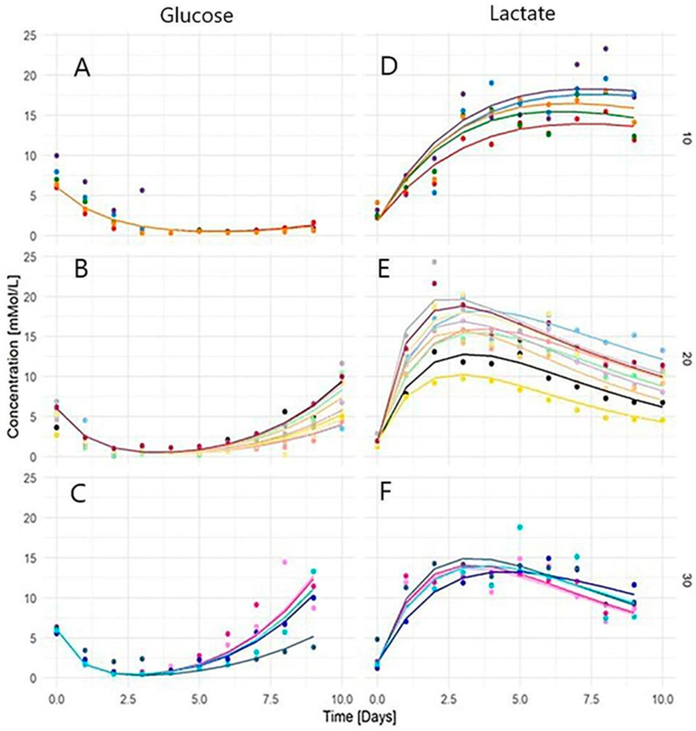
3.1. Glucose and Lactic Acid Kinetics and Temperature Dependence

Glu and Lac were quantified in human plasma collected from 20 donors. Concentration changes were measured for 10 consecutive days to study the kinetics of the two biomarkers at three different temperatures and to find a correlation with the postmortem interval. To achieve this, two equations, one each for Glu and Lac, were proposed, and the numerical values of the parameters in the equations were estimated. It was observed that ex vivo Glu and Lac concentrations in human plasma changed in a specific way over time, with the severity of this change being largely dependent on temperature.

More precisely, the kinetics of Glu stored at 10 °C (Figure 1A) were characterized by a decrease in concentration for four consecutive days. After this period, the concentrations were almost stable for the rest of the experiment. A different behavior was observed for the concentration of Glu stored at 20° (Figure 1B). In fact, the concentration of this marker decreased for three days, and it was stable for the following three days, from day four to day six. From day 7 to day 10, however, an increase in concentration was observed.

A very similar trend was observed in all the samples stored at 30 °C (Figure 1C). This time, the effect of temperature on the kinetics of Glu looked more dramatic. In fact, after three days, during which the concentration dropped, a sharp increase in plasmatic Glu was observed at day 5 until day 10. The upturn in concentration observed at 20 °C and 30 °C was always associated with the appearance of hemolysis in the samples; this phenomenon was faster at 30 °C and negligible at 10 °C. Hemolysis might have caused extra-cellular lysate to be released, which could explain the curve increment. Although this aspect needs to be investigated further, it was always present throughout the duration of the test.

As with Glu, the kinetics of Lac over time were affected by temperature. At 10 °C (Figure 1D), Lac was described by a constant increase, albeit characterized by fluctuations. At 20 °C (Figure 1E), Lac concentration rose for two days and then declined slowly for the remaining days. Lastly, when the temperature increased to 30 °C (Figure 1F), it was possible to observe a surge in Lac immediately after 24 h and a following stage of plateau persisting for approximately six days. After this time, the concentration of Lac finally dropped.

The Friedman test was employed to assess differences in Glu concentrations on different days (timepoints). We conclude that there were significant differences in Glu levels across different days; this finding underscores the dynamic nature of Glu concentrations over time (p-value < 0.001 at 10 °C; p-value < 0.001 at 20 °C; p-value < 0.001 at 30 °C). Similarly, it is important to note that time distinctly influences concentration for Lac across all three temperatures (p-value < 0.001 at 10 °C; p-value < 0.001 at 20 °C; p-value < 0.001 at 30 °C). After conducting a more detailed analysis, it also became evident that the natural logarithm of apparent rate constants for elimination, specifically lkel (p-value < 0.001) and lk2 (p-value < 0.001), exhibited notable sensitivity to changes in temperature; the same level of significance (p-value < 0.001) was observed for the constant lml. This finding underscores the significant relationship between the concentration of both Glu and Lac and temperature.

3.2. Parameters of Population Model

We created a combined mixed-effect model to understand the kinetics (rate of change) of the two biomarkers, Glu and Lac, over a period of time. Equations (1) and (2), previously mentioned in Section 2.3, represent the mathematical formulations associated with rate of change. The details, including numerical values of the parameters and their standard errors, are presented in

Table 1. Parameter estimates with non-linear mixed-effect regression for postmortem Glu and lactate kinetics and random effects.

Parameter Estimates
Lactate
Lmax	24.02 (1.86) **
IK1	−0.88 (0.16) **
Lo	1.88 (0.38) **
IK2ref	−1.98 (0.16) **
Ea_k2	35.43 (4.45) **
Parameter Estimates
Glucose
IKelref	−0.15 (0.09) *
Ea_kel	29.14 (8.21) **
Glus0	6.03 (0.25) **
ImIref	−5.93 (0.47) **
Ea_ml	79.80 (11.97) **
s	3.33 (0.22) **
Random Effects
σ s ID	0.16
σ Ik1 ID	0.44
σ Ik2 ID	0.35
AIC	1662.79
BIC	1731.48
Log likelihood	−814.40
Num. obs.	420
Num. groups	20

** p < 0.001, * p < 0.05.

below. The model aims to picture and describe the dynamic behavior of Glu and Lac over the specified timeframe of 10 days.

Each parameter was eventually defined as random or fixed within the population based on its variance relative to the parameter’s mean value. Using this information, different candidate models, each with different combinations of fixed and random parameters, were compared using the AIC and BIC scores and the log-likelihood testing for nesting comparisons before a final model was selected. Of all the different candidates, the best model with the lowest AIC and BIC score (Table 1 in bold) was the model with lk1, lk2 and s as random parameters and Glus0, lkel, lml, L0, and Lmax as fixed parameters.

Among the random parameters, we estimated value of −0.88 (p < 0.001) with a standard deviation of 0.44 for lk1, the estimate for lk2 was instead −1.98 (p < 0.001) with a standard deviation of 0.35. Lastly, the estimated value for the s parameter was 3.33 (p < 0.001) with a standard deviation of 0.16.

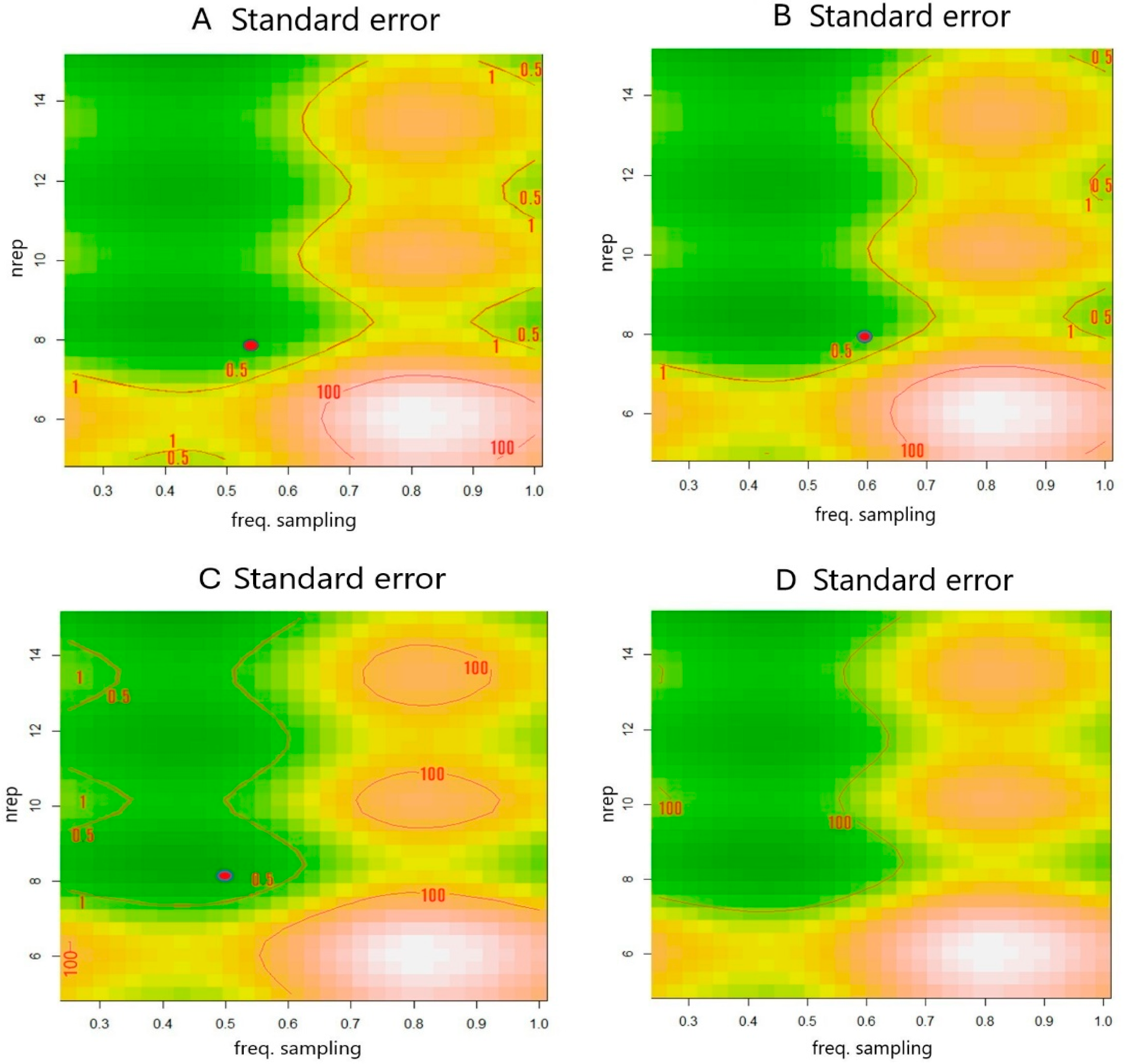
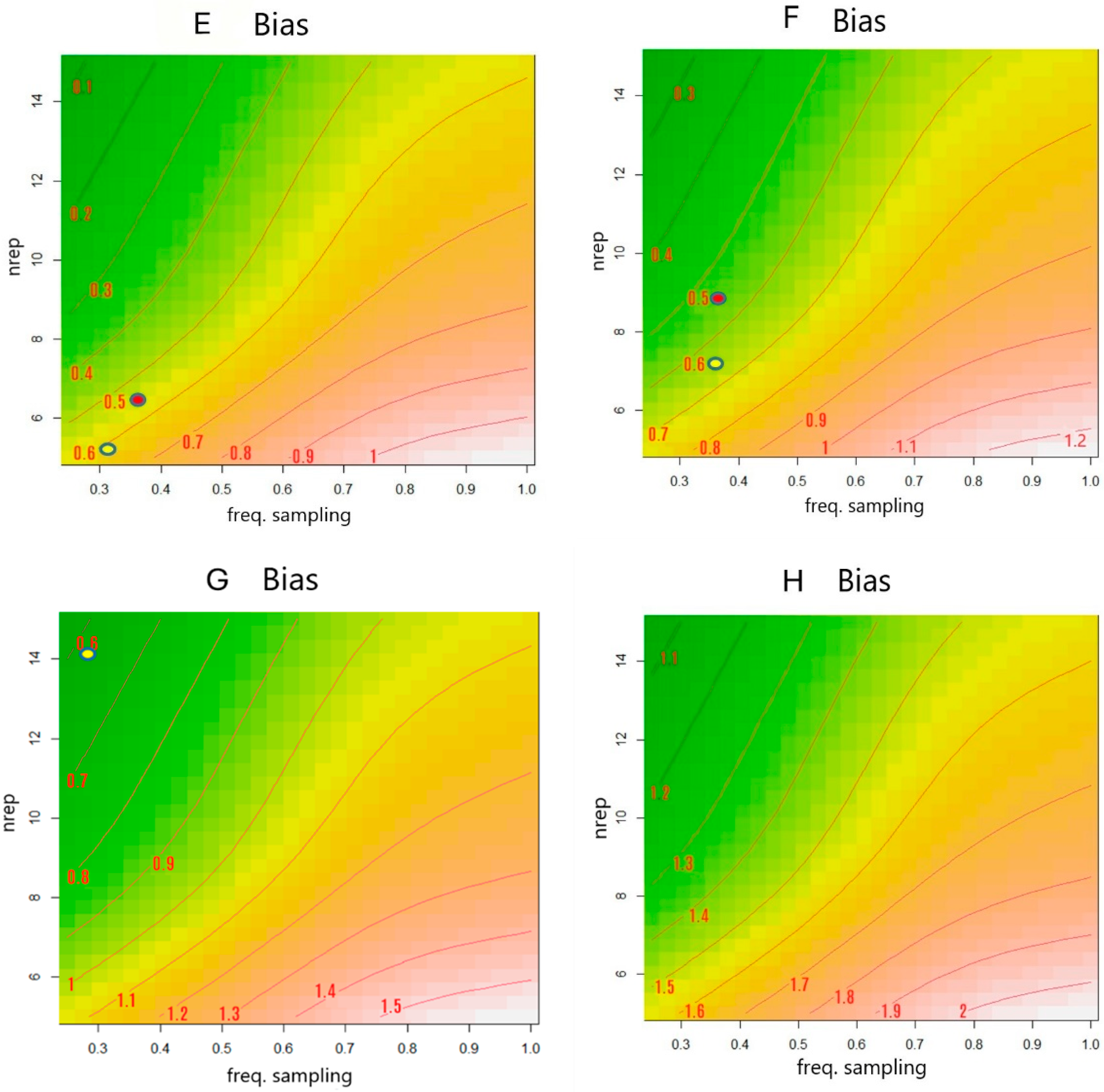
3.3. Best Set of Multiple Measurements That Delivered the Least Accuracy and Best Precision

One of the aims of this research was to find a sampling strategy consisting of multiple measurements of Glu and Lac in human blood to optimize the accuracy and precision of the PMI assessment. Bias, indicating the accuracy, was defined as the absolute value of the estimated PMI minus the true PMI, while the standard error was used to define precision. Multiple combinations of the number of days of sampling, the number of repetitions, and the frequency of sampling per day were included to assess this three-variable plan’s effect on PMI estimation. This process, performed with bootstrapping and non-linear least square regression, showed that increasing the number of days of sampling improved the assessment of PMI.

The results indicated that increasing the number of sampling days improved the precision of the PMI assessment. For instance, measuring Glu and Lac for 7 consecutive days (Figure 2A) achieved a precision estimate of 0.5 days with more than seven repetitions, with sample frequencies of around once per day being as effective as higher frequencies. Similar precision was observed with six consecutive sampling days (Figure 2B). However, with only 5 sampling days (Figure 2C), a precision of 0.5 days was achieved only with more than seven repetitions and a sampling frequency between 0.6 and 0.3 per day. A four-day sampling plan (Figure 2D) did not yield acceptable precision for any combination of sampling frequency and repetitions.

Similarly, accuracy increased with plans that included more sampling days. A seven-day sampling plan could achieve an accuracy of 0.5 with more than six repetitions and a sampling frequency of 0.3 per day (Figure 2E). Reducing the sampling frequency required a higher number of repetitions to maintain this level of accuracy. An accuracy of 0.5 was also attainable with six sampling days (Figure 2F), but it required at least eight repetitions and a sampling frequency above 0.4 per day. With five consecutive sampling days (Figure 2G), an acceptable accuracy of 0.6 was achievable only with 14 repetitions and a sampling frequency above 0.4 per day. A four-day sampling plan (Figure 2H) did not yield an acceptable accuracy, as the bias remained above 1 despite the high number of repetitions and sampling frequencies.

4. Discussion

There is a pressing need for of the use of biomarkers that can contribute to the delivery of a more precise and unbiased postmortem interval (PMI) estimate for forensic practices [31,32,33]. For this reason, researchers have recently tried to identify a suitable biomarker in blood samples. Biochemical markers in blood, such as histidine and hypoxanthine [34], nucleic acids [35], and specific proteins [36], as well as the observation of simple changes in blood color [37], have been studied to find a correlation with PMI. The biomarkers Glucose (Glu) and Lactic acid (Lac) are not currently used during postmortem examinations to assess PMI, yet their potential as PMI biomarkers has been proposed by authors such as Costa et al. [17] and Donaldson et al. [38]. However, all biomarkers used to make PMI estimations or determine other clinical effects will have some limitations. For example, a clinical parameter such as glycaemia after death is characterized by important fluctuations, because glycolysis proceeds even after death [39]; this makes it difficult to interpret Glu levels in postmortem blood [40]. Therefore, we selected the two most responsive biomarkers, Glu and Lac, for this study, based on data in a previous study of 4 blood biomarkers.

This biomarker study highlighted, among many other things, how changes in postmortem Glu and Lac did not follow a linear pattern, as previously confirmed by Trivedi et al. [41]. It was suggested that postmortem temperature-dependent hemolysis could be the most apparent cause of non-linearity in postmortem markers kinetics [42]; therefore, further studies are required to establish the intervening factors that affect the potential of Glu and Lac as blood biomarkers for PMI. We determined that non-linearity in kinetics, within a certain degree of complexity, should not be a reason to exclude a biomarker from the study.

Both Glu and Lac concentrations over time showed patterns characterized by significant intra-individual variability; for this reason, the mixed-effect model seemed to be the most appropriate statistical tool to describe this type of kinetics [43,44,45]. Our model, describing the kinetics of the two biomarkers, was defined by three random parameters exhibiting variability across the observed population of samples: lk1, lk2 and s. Meanwhile, five fixed parameters remained constant during the observation: Glus0, lkel, lml, L0 and Lmax. However, in subjects with potential alterations in the initial glucose value, Glus0 can be treated as a random parameter, requiring additional repetitions to account for the increased variability. Furthermore, the changes in the concentrations of both markers over time are strongly influenced by the temperature conditions at which the samples were tested, and this correlation was considered while modelling those time-dependent trends [46].

More important, our study showed that, in multiple readings of blood samples, the high frequency of measurements during the day with several repetitions improved the precision and accuracy of the PMI estimation. This is because the decrease and increase rates of Glu and Lac varied depending on the subject during the decomposition process. The computer simulation we ran showed that five consecutive days of sampling should deliver a good level of precision (as defined by the standard error) and accuracy (as defined by the bias), although a considerable number of repetitions and a high daily sampling frequency might be necessary to achieve this. Furthermore, a sampling plan with more than five consecutive days will increase precision and accuracy even further. On the other hand, after conducting sampling for a period shorter than five consecutive days, it was observed that low precision and accuracy led to inaccurate PMI estimations, underscoring the fact that, given the available data, a single-point measurement is entirely ineffective. By evaluating various sequences of repetitions and sampling frequencies, we identified the optimal combination to achieve a bias and standard error of approximately 0.5 within five consecutive days of measurement. Finally, to ensure precision and accuracy, fewer sampling frequencies per day and repetitions are needed if the number of test days is increased to six or seven.

While the study was conducted via the biochemical testing of blood biomarkers, the findings provide valuable insights for developing a more accurate and reliable method for estimating PMI that can be used in conjunction with or as an alternative to pathological investigations. Our research suggests that, by collecting more than one measurement of the same sample, it is possible to generate a more accurate estimate of the PMI. A PMI estimate could be delivered with low bias and good precision if these three factors are considered: (1) the number of samplings per day, (2) the frequency of measurements during the day, and (3) the number of repetitions. However, it is not clear whether these factors would be still viable during a real PMI estimate performed by a pathologist during an autopsy, nor how a postmortem circulation might influence the identification of a suitable site of blood sampling during postmortem examination [47]. Furthermore, while this sampling method could mitigate the problems of temperature dependency and inter-individual variation, we still do not know the effect of other factors such as pre-existing conditions [48] and the manner of death [49]. An in situ study could shed more light on the apparent correlation between Glu, Lac and other factors influencing the PMI to further develop our hypothesis and alternative approaches for PMI determination. Moreover, this methodology could be applied retrospectively to investigate discrepancies between estimated and recorded times of death. Once validated, it may complement traditional pathology in cases where physical indicators are unreliable, enhancing PMI estimations.

In conclusion, the measurement of Glu and Lac levels in blood samples could potentially be useful for estimating the PMI. However, an important aspect of this alternative approach is not the biomarkers themselves, but the methodology, which uses multiple readings, frequent sampling throughout the day, and sufficient repetitions, as shown in our mixed-effect mathematical modelling. This method could serve as a tool for improving PMI estimations, as it could potentially be applied to any biomarker while also considering non-linearity and intra-individual variation. While this approach might look promising, we acknowledge the need for improvements, particularly in adapting it to more realistic conditions or validation in situ.

References

1. Kaliszan, M.; Hauser, R.; Kernbach-Wighton, G. Estimation of the time of death based on the assessment of post mortem processes with emphasis on body cooling. Legal Med. 2009, 11, 111–117. [Google Scholar] [CrossRef] [PubMed]
2. Shrestha, R.; Kanchan, T.; Krishan, K. Methods of Estimation of Time Since Death. In StatPearls [Internet]; StatPearls: Treasure Island, FL, USA, 2023. Available online: https://www.ncbi.nlm.nih.gov/books/NBK549867/ (accessed on 6 June 2024).
3. Saukko, P.; Knight, B. Knight’s Forensic Pathology, 3rd ed.; Hodder Arnold: London, UK, 2004; p. 64. [Google Scholar]
4. Swain, R.; Kumar, A.; Sahoo, J.; Lakshmy, R.; Gupta, S.K.; Bhardwaj, D.N.; Pandey, R.M. Estimation of post-mortem interval: A comparison between cerebrospinal fluid and vitreous humour chemistry. J. Forensic Leg. Med. 2015, 36, 144–148. [Google Scholar] [CrossRef] [PubMed]
5. Sacco, M.A.; Cordasco, F.; Scalise, C.; Ricci, P.; Aquila, I. Systematic Review on Post-Mortem Protein Alterations: Analysis of Experimental Models and Evaluation of Potential Biomarkers of Time of Death. Diagnostics 2022, 12, 1490. [Google Scholar] [CrossRef]
6. Ferreira, M.T.; Cunha, E. Can we infer post mortem interval on the basis of decomposition rate? A case from a Portuguese cemetery. Forensic Sci. Int. 2013, 226, 298.e1–298.e6. [Google Scholar] [CrossRef]
7. Nolan, A.-N.; Mead, R.J.; Maker, G.; Speers, S.J. A review of the biochemical products produced during mammalian decomposition with the purpose of determining the post-mortem interval. Aust. J. Forensic Sci. 2019, 52, 477–488. [Google Scholar] [CrossRef]
8. Yang, T.; You, M.; Zhang, H.; Zhang, F.; Bai, R.; Chang, L.; Di, S.; Guo, Z.; Lu, D.; Wang, X.; et al. Estimation of the Postmortem Interval by Measuring Blood Oxidation-reduction Potential Values. J. Forensic Sci. Med. 2016, 2, 8–11. [Google Scholar] [CrossRef]
9. Kumar, S.; Verma, A.K. Estimation of postmortem interval using the data of insulin level in the cadaver’s blood. Data Brief 2016, 7, 354–356. [Google Scholar] [CrossRef]
10. Nishida, A.; Funaki, H.; Kobayashi, M.; Tanaka, Y.; Akasaka, Y.; Kubo, T.; Ikegaya, H. Blood creatinine level in postmortem cases. Sci. Justice 2015, 55, 195–199. [Google Scholar] [CrossRef]
11. Castillo-Peinado, L.S.; Luque de Castro, M.D. An overview on forensic analysis devoted to analytical chemists. Talanta 2017, 167, 181–192. [Google Scholar] [CrossRef]
12. Whitney, A.R.; Diehn, M.; Popper, S.J.; Alizadeh, A.A.; Boldrick, J.C.; Relman, D.A.; Brown, P.O. Individuality and variation in gene expression patterns in human blood. Proc. Natl. Acad. Sci. USA 2003, 100, 1896–1901. [Google Scholar] [CrossRef]
13. Gao, Y.; Liu, Y.; He, J.; Zhang, Y.; Wang, T.; Wu, L.; Sun, N.; Fang, T.; Mao, H.; Tang, N.J.; et al. Effects of heat waves and cold spells on blood parameters: A cohort study of blood donors in Tianjin, China. Environ. Health Prev. Med. 2024, 29, 25. [Google Scholar] [CrossRef] [PubMed]
14. Matrai, A.A.; Varga, G.; Tanczos, B.; Barath, B.; Varga, A.; Horvath, L.; Bereczky, Z.; Deak, A.; Nemeth, N. In vitro effects of temperature on red blood cell deformability and membrane stability in human and various vertebrate species. Clin. Hemorheol. Microcirc. 2021, 78, 291–300. [Google Scholar] [CrossRef]
15. Meurs, J.; Krap, T.; Duijst, W. Evaluation of postmortem biochemical markers: Completeness of data and assessment of implication in the field. Sci. Justice 2019, 59, 177–180. [Google Scholar] [CrossRef]
16. Kost, G.J.; Nguyen, T.H.; Tang, Z. Whole-blood glucose and lactate: Trilayer biosensors, drug interference, metabolism, and practice guidelines. Arch. Pathol. Lab. Med. 2000, 124, 1128–1134. [Google Scholar] [CrossRef]
17. Costa, I.; Carvalho, F.; Magalhães, T.; Guedes de Pinho, P.; Silvestre, R.; Dinis-Oliveira, R.J. Promising blood-derived biomarkers for estimation of the postmortem interval. Toxicol. Res. 2015, 4, 1443–1452. [Google Scholar] [CrossRef]
18. I Muñoz, J.; Costas, E.; Rodrĺguez-Calvo, M.S.; Suárez-Peñaranda, J.M.; López-Rivadulla, M.; Concheiro, L. A high-performance liquid chromatography method for hypoxanthine determination in vitreous humour: Application to estimation of post mortem interval. Hum. Exp. Toxicol. 2006, 25, 279–281. [Google Scholar] [CrossRef] [PubMed]
19. Cordeiro, C.; Ordóñez-Mayán, L.; Lendoiro, E.; Febrero-Bande, M.; Vieira, D.N.; Muñoz-Barús, J.I. A reliable method for estimating the postmortem interval from the biochemistry of the vitreous humor, temperature and body weight. Forensic Sci. Int. 2019, 295, 157–168. [Google Scholar] [CrossRef]
20. Rodrigo, M.R. A Nonlinear Least Squares Approach to Time of Death Estimation Via Body Cooling. J. Forensic Sci. 2016, 61, 230–233. [Google Scholar] [CrossRef]
21. Weiser, M.; Roggendorf, M.; Schuck, J. Optimal design of experiments for estimating the time of death in forensic medicine. Inverse Probl. 2018, 34, 125005. [Google Scholar] [CrossRef]
22. Collins, S.; Maestrini, L.; Hui, F.K.C.; Stuart, B.; Ueland, M. The use of generalized linear mixed models to investigate postmortem lipids in textiles. iScience 2023, 26, 107371. [Google Scholar] [CrossRef]
23. Beneke, R.; Hütler, M.; Jung, M.; Leithäuser, R.M. Modeling the blood lactate kinetics at maximal short-term exercise conditions in children, adolescents, and adults. J. Appl. Physiol. 2005, 99, 499–504. [Google Scholar] [CrossRef]
24. Flores-Bazán, F.; Hadjisavvas, N.; Lara, F.; Montenegro, I. First- and Second-Order Asymptotic Analysis with Applications in Quasiconvex Optimization. J. Optim. Theory Appl. 2016, 170, 372–393. [Google Scholar] [CrossRef]
25. Murthy, D.N.P.; Xie, M.; Jiang, R. Weibull Models; John Wiley & Sons, Inc.: Hoboken, NJ, USA, 2004. [Google Scholar]
26. Pinheiro, J.; Bates, D.; DebRoy, S.; Sarkar, D.; EISPACK authors; Heisterkamp, S.; Van Willigen, B.J.; Ranke, J.; R Core Team. nlme: Linear and nonlinear mixed effects models. R Package Version 2017, 3, 274. [Google Scholar]
27. Haralampu, S.G.; Saguy, I.; Karel, M. Estimation of Arrhenius model parameters using three least squares methods. J. Food Sci. 1985, 9, 129–143. [Google Scholar] [CrossRef]
28. Schoenly, K.; Goff, M.L.; Wells, J.D.; Lord, W.D. Quantifying statistical uncertainty in succession-based entomological estimates of the postmortem interval in death scene investigations: A simulation study. Am. Entomol. 1996, 42, 106–112. [Google Scholar] [CrossRef]
29. Padfield, D.; Matheson, G. nls.multstart: Robust Non-Linear Regression using AIC Scores. R Package Version 2018, 1, 1–5. Available online: https://CRAN.R-project.org/package=nls.multstart (accessed on 15 April 2025).
30. Nahm, F.S. Nonparametric statistical tests for the continuous data: The basic concept and the practical use. Korean J. Anesthesiol. 2016, 69, 8–14. [Google Scholar] [CrossRef]
31. Garg, S.P.; Garg, V. Serum enzymes changes after death & its correlation with time since death. J. Indian Acad. Forensic Med. 2010, 32, 355–357. [Google Scholar]
32. Go, A.; Shim, G.; Park, J.; Hwang, J.; Nam, M.; Jeong, H.; Chung, H. Analysis of hypoxanthine and lactic acid levels in vitreous humor for the estimation of post-mortem interval (PMI) using LC–MS/MS. Forensic Sci. Int. 2019, 299, 135–141. [Google Scholar] [CrossRef]
33. Rognum, T.; Holmen, S.; Musse, M.; Dahlberg, P.; Stray-Pedersen, A.; Saugstad, O.; Opdal, S. Estimation of time since death by vitreous humor hypoxanthine, potassium, and ambient temperature. Forensic Sci. Int. 2016, 262, 160–165. [Google Scholar] [CrossRef]
34. Szeremeta, M.; Samczuk, P.; Pietrowska, K.; Kowalczyk, T.; Przeslaw, K.; Sieminska, J.; Kretowski, A.; Niemcunowicz-Janica, A.; Ciborowski, M. In vitro animal model for estimating the time since death with attention to early postmortem stage. Metabolites 2023, 13, 26. [Google Scholar] [CrossRef] [PubMed]
35. Fujihara, J.; Takinami, Y.; Kawai, Y.; Kimura-Kataoka, K.; Takeshita, H. Comparison of serum cell-free DNA between postmortem and living samples. Clin. Chim. Acta 2021, 519, 255–259. [Google Scholar] [CrossRef] [PubMed]
36. El-Din, E.A.A.; Ahmed, S.M.; El Shafei, D.A.; Mostafa, H.E.-S. Implication of high-mobility group box-1 and skin post mortem changes in estimation of time passed since death: Animal and human study. Legal Med. 2021, 53, 101949. [Google Scholar] [CrossRef] [PubMed]
37. Usumoto, Y.; Kudo, K.; Tsuji, A.; Ihama, Y.; Ikeda, N. Predictive equation to estimate post-mortem interval using spectrophotometric blood-colour values. Med. Sci. Law 2019, 59, 36–41. [Google Scholar] [CrossRef]
38. Donaldson, A.E.; Lamont, I.L. Biochemistry changes that occur after death: Potential markers for determining post-mortem interval. PLoS ONE 2013, 8, 1–10. [Google Scholar] [CrossRef]
39. Palmiere, C.; Mangin, P.; Augsburger, M. Postmortem biochemical investigation results in situations of fatal mechanical compression of the neck region. Legal Med. 2018, 30, 59–63. [Google Scholar] [CrossRef]
40. Palmiere, C. Postmortem diagnosis of diabetes mellitus and its complications. Croat. Med. J. 2015, 56, 181–193. [Google Scholar] [CrossRef]
41. Trivedi, D.; Narayana, K.S. Postmortem blood glucose level: How useful to envisage the time since death. Int. J. Clin. Biochem. Res. 2015, 2, 61–64. [Google Scholar]
42. Woydt, L.; Bernhard, M.; Kirsten, H.; Burkhardt, R.; Hammer, N.; Gries, A.; Dreßler, J.; Ondruschka, B. Intra-individual alterations of serum markers routinely used in forensic pathology depending on increasing post-mortem interval. Sci. Rep. 2018, 8, 1–12. [Google Scholar] [CrossRef]
43. Van Dongen, H.P.; Olofsen, E.; Dinges, D.F.; Maislin, G. Mixed-model regression analysis and dealing with interindividual differences. Methods Enzymol. 2004, 384, 139–171. [Google Scholar] [CrossRef]
44. Anderson, B.J.; Allegaert, K.; Holford, N.H.G. Population clinical pharmacology of children: Modelling covariate effects. Eur. J. Pediatr. 2006, 165, 819–829. [Google Scholar] [CrossRef]
45. Allegaert, K.; Peeters, M.Y.; Verbesselt, R.; Tibboel, D.; Naulaers, G.; de Hoon, J.N.; Knibbe, C.A. Inter-individual variability in propofol pharmacokinetics in preterm and term neonates. Br. J. Anaesth. 2007, 99, 864–870. [Google Scholar] [CrossRef] [PubMed]
46. Yang, M.; Li, H.; Yang, T.; Ding, Z.; Wu, S.; Qiu, X.; Liu, Q. A study on the estimation of postmortem interval based on environmental temperature and concentrations of substances in vitreous humor. J. Forensic Sci. 2018, 63, 745–751. [Google Scholar] [CrossRef] [PubMed]
47. Abdelaal, G.M.M.; Hegazy, N.I.; Etewa, R.L.; Elmesallamy, G.E.A. Postmortem redistribution of drugs: A literature review. Forensic Sci. Med. Pathol. 2024, 20, 1483–1490. [Google Scholar] [CrossRef] [PubMed]
48. Zilg, B.; Alkass, K.; Berg, S.; Druid, H. Postmortem identification of hyperglycemia. Forensic Sci. Int. 2009, 185, 89–95. [Google Scholar] [CrossRef]
49. Chen, J.H.; Michiue, T.; Inamori-Kawamoto, O.; Ikeda, S.; Ishikawa, T.; Maeda, H. Comprehensive investigation of postmortem glucose levels in blood and body fluids with regard to the cause of death in forensic autopsy cases. Leg. Med. 2015, 17, 475–482. [Google Scholar] [CrossRef]
Figure 1. Kinetics of Glu (AC) and Lac (DF) concentrations at 10 °C (A,D), 20 °C (B,E), and 30 °C (C,F). Each color in the graphic represents an individual longitudinal study and each dot a sampling instance. The continuous lines show the model fitting for each individual.
Forensicsci 05 00017 g001
Figure 2. Estimated PMI standard error (AD) and bias (EH) after analyzing the sample for seven (A,E), six (B,F), five (C,G), and four (D,H) consecutive days. The red iso lines delimit the areas of the graph where it is possible to obtain that value of bias or standard error associated with that specific number of replicates and frequency of sampling. The red dot indicates the areas where it is possible to obtain a value of 0.5 for both bias and the standard error. The yellow dot indicates the areas where it is possible to obtain a value of 0.6 for both bias and standard error.
Forensicsci 05 00017 g002aForensicsci 05 00017 g002b