Whole Slide Image Understanding in Pathology: What Is the Salient Scale of Analysis?

Abstract

Background: In recent years, there has been increasing research in the applications of Artificial Intelligence in the medical industry. Digital pathology has seen great success in introducing the use of technology in the digitisation and analysis of pathology slides to ease the burden of work on pathologists. Digitised pathology slides, otherwise known as whole slide images, can be analysed by pathologists with the same methods used to analyse traditional glass slides. Methods: The digitisation of pathology slides has also led to the possibility of using these whole slide images to train machine learning models to detect tumours. Patch-based methods are common in the analysis of whole slide images as these images are too large to be processed using normal machine learning methods. However, there is little work exploring the effect that the size of the patches has on the analysis. A patch-based whole slide image analysis method was implemented and then used to evaluate and compare the accuracy of the analysis using patches of different sizes. In addition, two different patch sampling methods are used to test if the optimal patch size is the same for both methods, as well as a downsampling method where whole slide images of low resolution images are used to train an analysis model. Results: It was discovered that the most successful method uses a patch size of 256 × 256 pixels with the informed sampling method, using the location of tumour regions to sample a balanced dataset. Conclusion: Future work on batch-based analysis of whole slide images in pathology should take into account our findings when designing new models.

1. Introduction

Digital pathology is a relatively new area of pathology wherein specimen slides are digitised for analysis, minimising the time needed for the diagnostic process of a patient. These digital tissue samples are called whole slide images (WSIs) and can be utilised similarly to glass pathology slides in the identification of disease. This technology has the potential to become routine in clinical pathology settings and has paved the way for the possibility of automated WSI classification using machine learning architectures.

The main concept behind the automated analysis of WSIs is to imitate the process that a pathologist ordinarily follows to complete analysis of a WSI. Often, the overarching goal of the analysis is to identify the presence of tumourous tissue in a WSI. As the nature of the analysis is to mimic the pathologists’ cognitive process, deep learning methods are best suited to this task. In particular, deep learning methods have proven vastly superior to traditional machine learning models in extracting nuanced patterns from highly complex and high-dimensional data. For example, they have been widely used to learn from training images how to identify the presence and localize tumorous tissue in a WSI [1]. Unfortunately, due to the size of WSIs (often several gigapixels [2]), it is not possible to input the raw images into a network. Different methods have been researched to overcome this, namely downsampling of WSIs and patch extraction [3,4].

The focus of this work is on the patch-based method of WSI analysis. Patch-based methods involve splitting the WSIs into small patches and extracting a subset of these patches to input into a neural network [2,3]. Patch extraction can be performed using various sampling methods, two of which were implemented as part of this work. The patch-based method is the commonly preferred alternative to the downsampling method which retrieves lower resolution versions of the WSI that can be processed as entire images by a neural network [3,4].

Patch-based methods are common in the classification of WSIs. However, there is little research into the effect of patch size on the accuracy of the classification. A majority of the related work uses a relatively small patch size, typically around 256 × 256 pixels [5,6,7]. This is largely a choice borne out initially out of practical computational constraints and subsequently adopted for the sake of uniformity, ease of comparison with previous work, and tradition. No work has examined whether this choice is optimal and indeed any longer sensible, given the improvements in computational power—the use of small patches limits the amount of spatial information that is exploited which inevitably affects overall performance. Hence, the present work aims to implement a patch-based WSI analysis method in order to evaluate the effect of patch size on the automatic analysis of WSIs.

Four patch sizes were evaluated for the initial random sampling method (256, 384, 512, and 786), and three patch sizes were tested with the informed sampling method (256, 512, and 1024). Figure 1 shows the level of detail present in each of the patch sizes. Only the largest downsampling factor was used for the downsampling method.

2. Related Work

2.1. Introduction to Digital Pathology

Pathology is a field of medicine related to the diagnosis and staging of diseases, including cancer. Since the 1800s [8], pathologists have carried out this work by examining specimen on glass slides using a microscope. However, for the past few decades there has been increasing research in the digitisation of this process, resulting in the subfield of digital pathology. This began with the introduction of WSI scanners in the early 2000s [9]. These scanners produce WSIs, high-resolution images of glass pathology slides which contain billions of pixels and are around 2 gigabytes in size [10]. The use of WSIs as a replacement for the traditional glass slides means specimens can be displayed on large screens, viewed in locations outside the hospital and laboratory environment, and shared between pathologists and experts. These possibilities help to improve accuracy of diagnosis, allow for collaboration between medical personnel, and create a flexible work environment [9,10,11]. Another use of WSIs in digital pathology is for the automation of the analysis of WSIs, using deep learning. Applying this in a clinical setting would ease the workload of pathologists, reduce wait times, and standardise the analysis of pathology slides [5]. However, the nature of WSIs, the size, high morphological variance and artefacts present, prevent the use of conventional deep learning methods [5].

Research and advancements in digital pathology have positively impacted the healthcare industry; the ability to digitise pathology slides has eliminated the need for costly storage of glass slides, and allows for remote pathological analysis and faster diagnoses, without sacrificing any accuracy in the pathologists’ results [12,13]. However, some of the concerns that occur in the analysis of pathology slides are not solved by the use of WSIs. The manual analysis of WSIs still remains to be a time-consuming process and there is no standardisation between pathologist’s analyses or different pathologists’ results. To solve this, research continues into the automation of WSI classification. By using machine learning algorithms to aid with the analysis, the time taken for this process can be reduced and there can be a level of standardisation between outcomes [5,12,14,15]. The computational analysis of WSIs also has the ability to account for more morphological information than a human can which leads to a better accuracy of diagnoses [4].

Future advances in digital pathology show a great deal of promise, but progress is slowed by various barriers, including ethical concerns and regulations [9]. In the near future, it is likely that this technology will be slowly introduced into the diagnostic process, aiding pathologists by analysing slides and prioritising those that the algorithm indicates contain disease [12,16,17]. The introduction of the Grand Challenges has fast-tracked research in this field, providing datasets and creating an environment for researchers to submit their work. Recent diagnostic models have shown a great deal of promise, performing better than pathologists, mimicking a time-pressured environment, in the diagnosis and staging of disease from imaging [18].

2.2. Analysis of Whole Slide Images

Deep learning algorithms have been successfully used for the classification of WSIs, producing results similar to that of pathologists. The automation of analysis of WSIs has many advantages over the traditional manual annotation of glass pathology slides. However, there are barriers to overcome in achieving a successful implementation for this process. In recent years, digital pathology research has focused on methods to overcome these issues, with the most significant being the large size of WSIs and a lack of annotated training data. The lack of data is due to the annotation process performed by pathologists being time-consuming and therefore yielding only a small amount of available training data.

Problems with Computational Analysis of Whole Slide Images

WSIs contain billions to trillions of pixels per image and, on average, range from 1 to 4 GB in size [9]. This makes the use of conventional deep learning algorithms computationally expensive and impractical [3,4,5,12,13,19]. There are two common methods for dealing with this issue: downsampling and patch extraction. Downsampling involves scaling down the WSI until it contains much fewer pixels and can be analysed by a conventional deep learning algorithm [4,12,20,21]. This method is not desirable as the process results in a significant loss of fine detail from the image, affecting the classification accuracy [6,15,19,22]. Patch extraction splits the WSI into many small patches that can be analysed individually by a deep learning algorithm and, using the patch-level classifications, produce a slide-level classification [4,12]. Patch-based methods usually involve assigning the relevant slide-level label to all patches in the training data. This can be misleading as some patches from tumour-containing slides will not contain any diseased tissue themselves, meaning the model is being given false information [12]. There is also a loss of spatial information using a patch-based method, the relationship between patches and the global information is lost. Therefore this method assumes that slide level analysis can be extrapolated from patch-level information [4]. Despite the loss of spatial information using patch-based methods, this method is preferable over downsampling as it retains more morphological information and detail from the WSI [4].

A major bottleneck in the use of deep learning for the analysis of WSIs is the insufficiency of training data. WSIs have multiple levels at which annotations can be performed; pixel-level, patch-level, slide-level, lesion-level, and patient-level. Ideally, the training data for an analysis model will contain patch-level annotations to produce results comparable to experts [5]. However, manual annotations must be carried out by pathologists which is an expensive and time-consuming process, particularly at the more detailed pixel- and patch-levels where the pathologist annotates the exact location of any disease [4,13,22,23]. This impedes the use of fully supervised models using patch-based labelling which has the advantage of predicting where disease is present in an image [16]. As an alternative, weakly supervised learning methods are being widely adopted in the analysis of WSIs [13]. These methods use only slide-level annotations, describing if there is any disease present in a WSI, but not where in the image the disease is [12], to train the model.

The above two problems are the most significant barriers to the computational analysis of WSIs. However, there are also many smaller issues that must be tackled to build a successful model. Depending on the laboratory, scanner, and a number of other factors, there can be a significant amount of stain variation between WSIs and various artefacts [7,10,15,24]. Pathologists adapt to ignore these variations and distractions. An AI model is not capable of doing this which can affect the results of the classification [5]. To counteract the stain variation, colour normalisation can be applied to the WSIs during pre-processing [7,24], and the use of, for example, image filters can eliminate artefacts [5]. The extraction of features for classification can be difficult as WSIs can contain a lot of heterogeneity and there is sometimes little noticeable difference between disease and normal tissue [15,25]. This makes it tricky for the model to learn disease patterns and is amplified by the previously mentioned issue of a lack of WSI annotations as the location of disease is not specified to the model [22]. There also tends to be significant class imbalance with a benign/normal tissue class containing many more samples compared to a malignant/disease tissue class. A reason for this is that all slides, malignant, benign, and other, usually contain some normal tissue, whereas slides which are labelled as benign contain no disease tissue [13]. This issue can be minimised by, prior to analysis, performing data augmentation which involves applying different geometric transformations to the images [19]. Other methods include hard negative mining, where false positives are added to the training data, and sampling patches using patch-level annotations rather than random sampling; although these rely on the availability of patch-level annotations [5].

2.3. Patch-Based Whole Slide Image Analysis

Much of the current research in digital pathology focuses on patch-based methods for the analysis of WSIs, however, the work varies on pre-processing techniques, including patch extraction, model architecture, and classification. These processes are outlined below. The goal of these techniques is to optimise the accuracy of the model in predicting the presence of disease; this article will focus on the optimisation of patch size.

• Pre-processing: Before the data is fed into a model, pre-processing must be applied first. For patch-based WSI analysis, there are four main steps for pre-processing:

  (a)

  Tissue segmentation detects unwanted areas of WSIs, such as any background or blurry areas. These areas are irrelevant in the analysis of the tissue and are usually large regions so take up a significant amount of computational power to process [10].

  (b)

  Colour normalisation alters the distribution of colour values in an image to standardise the range of colour used. In the case of WSIs, this ensures that only relevant colour differences appear between slides. This is essential in the pre-processing of WSIs as it minimises the stain variation between images which can lead to bias in the training data and affect the results [7,19].

  (c)

  Patch extraction involves taking square patches, often 256 × 256 pixels in size, from the WSI for patch-level analysis [5,6,7]. This step of pre-processing has many variables that can be optimised; patch size, magnification/resolution level, sampling method, and whether patches are tiled or overlapping. This is done due to the large size of WSIs and the limits of computational power to deal with images of this size.

  (d)

  Data augmentation is the transformation of training data to new training data. This prevents overfitting and can be used to deal with severe class imbalance.

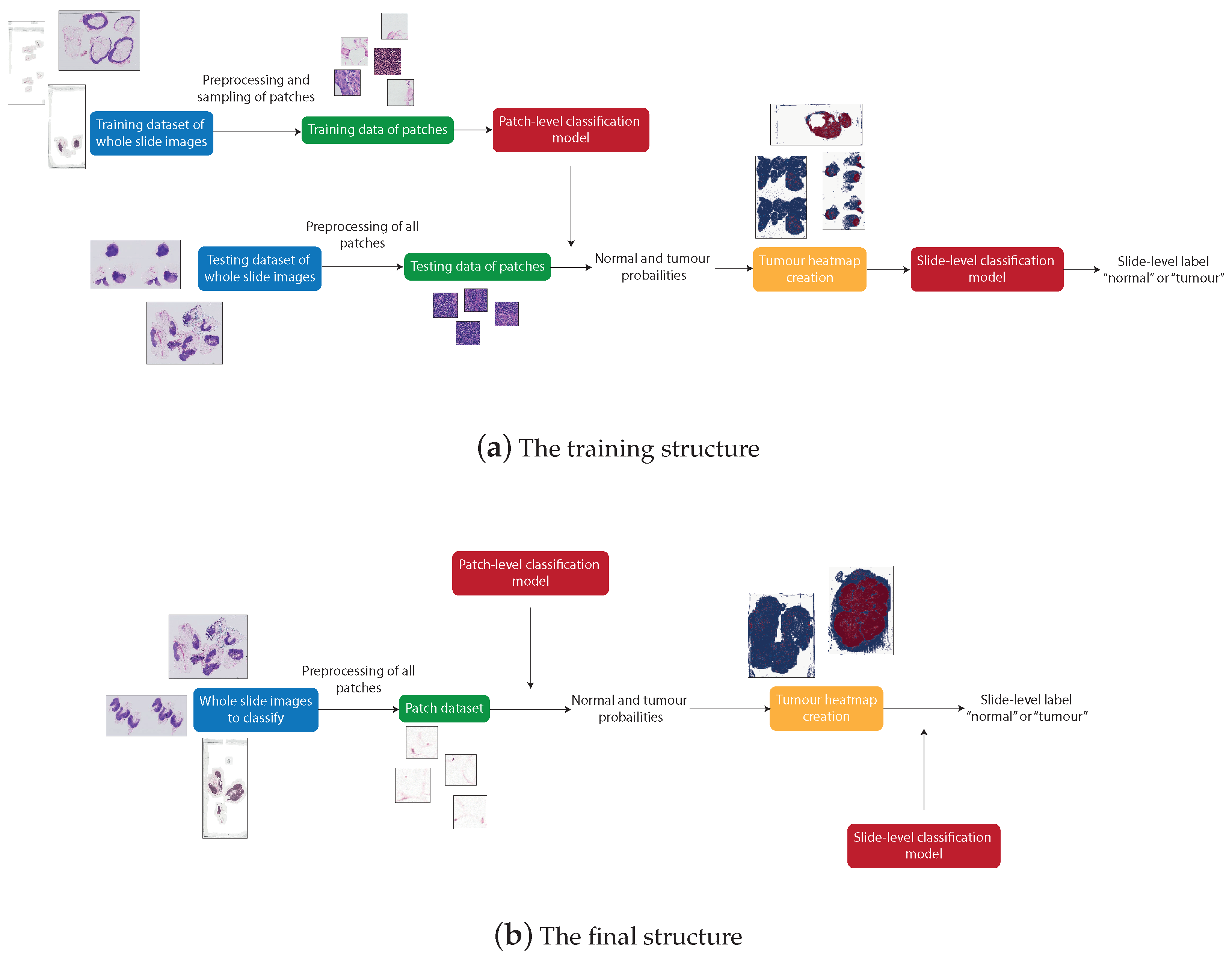
• Architecture: Commonly, convolutional neural networks (CNNs) are used for the analysis of WSIs. Due to the insufficiency of training data, these models are often weakly supervised. A form of weakly supervised learning that can be used is multiple-instance learning (MIL). This is suitable for data where a class label is assigned to many instances, for example a slide label assigned to patches of that slide [13]. Originally, this algorithm would apply max pooling to the instances, meaning that if disease is predicted to be in one patch, the whole slide is predicted to be in the disease class [13].
• Classification: For the analysis of WSIs, there are two classifications, patch-level and slide-level classification [7]. Predictions for patches are aggregated to produce slide-level classifications. Heatmaps are often used to display the distribution of results for the patches in a slide which often correlates with a pathologist’s annotation of the slide.

2.3.1. Techniques Used in Related Work

Wang et al. [26] use a CNN to make patch-level classifications which are then used to produce a probability heatmap to predict the slide-level classification. WSI background is removed to prevent unnecessary computation using a threshold segmentation method with Otsu’s algorithm. The patches used for classification are extracted at 256 × 256 pixels at 40× magnification level.

Hou et al. [3] used a CNN for patch-level classification followed by a decision fusion model. 500 × 500 pixel patches extracted at 20× and 5× magnification levels were used to train the model. Any patches that included too much unnecessary tissue or blood were discarded. Three kinds of data augmentation were applied to the patches to prevent overfitting. This included rotation and reflection of part of each patch and colour augmentation to affect the Hematoxylin and Eosin (H&E) stain.

Cruz-Roa et al. [27] downsampled the WSIs by a factor of 16:1 and tiled them into 100 × 100 pixel patches using grid sampling, discarding any patches that were largely fatty tissue or background. These patches were then converted to YUV colour space and normalised and then input into a 3-layer CNN which outputs the log likelihoods of the patch being disease or not. The outputs were transformed to be interpreted as probabilities and used to form a probability map for each WSI.

Yue et al. [19] used the Reinhard normalisation to minimise stain variation on the WSIs. Each WSI is downsampled and normalised before patches of size 224 × 224 pixels are extracted. The data augmentation techniques, rotations, reflections, Gaussian blur, and all-channel multiplication, were applied to the data to prevent overfitting and to help with class imbalance.

Ruan et al. [28] first used a fixed-level threshold segmentation method to remove background from the WSIs. Patches were sampled using a novel adaptive sampling method at both the 20× and 40× magnification levels and were chosen to be 256 × 256 pixels. Sampling at alternative magnification levels was tested and a combination of sampling at 20× and 40× magnification was shown to give the best results.

Rodriguez et al. [7] performed a systematic review of AI used in the analysis of WSIs. All 26 studies included in the review used patch-based methods, with varied other pre-processing techniques. A majority used tissue segmentation to remove unwanted regions of the WSIs, and the most common technique used was a threshold. Colour normalisation was only used in six of the studies, with techniques of colour deconvolution and simple normalisation. Data augmentation was widely used with a variety of methods, including rotations, flipping, and colour augmentations. Most studies used deep learning models for patch-level classification, with many different methods used for slide-level classification, with some simply opting for the most common class and others using more complex deep learning models.

Mohammadi et al. [13] implemented an extended MIL method for multi-class classification. WSIs are downsampled and the tissue is segmented to eliminate unnecessary background in the image and converted to HSV colour space. Non-overlapping patches of size 256 × 256 pixels are taken from only the segmented tissue at magnification level 0.

Fell et al. [16] used a fully supervised CNN to predict the probability of each patch from a WSI containing disease. The outputs from the CNN were then aggregated to form a heatmap for the WSI to be used as input to a slide-level classification model. Colour normalisation and aggregation were not used in an attempt to increase variation within the data for generalisation. Background was removed from the thumbnail by applying greyscale and removing any values over a threshold. Patches were extracted at the highest resolution level, level 0, and multiple patch sizes were tested for optimisation, 256 × 256 pixels, 512 × 512 pixels, and 1024 × 1024 pixels. The largest patch size, 1024 × 1024 pixels, was chosen for this model.

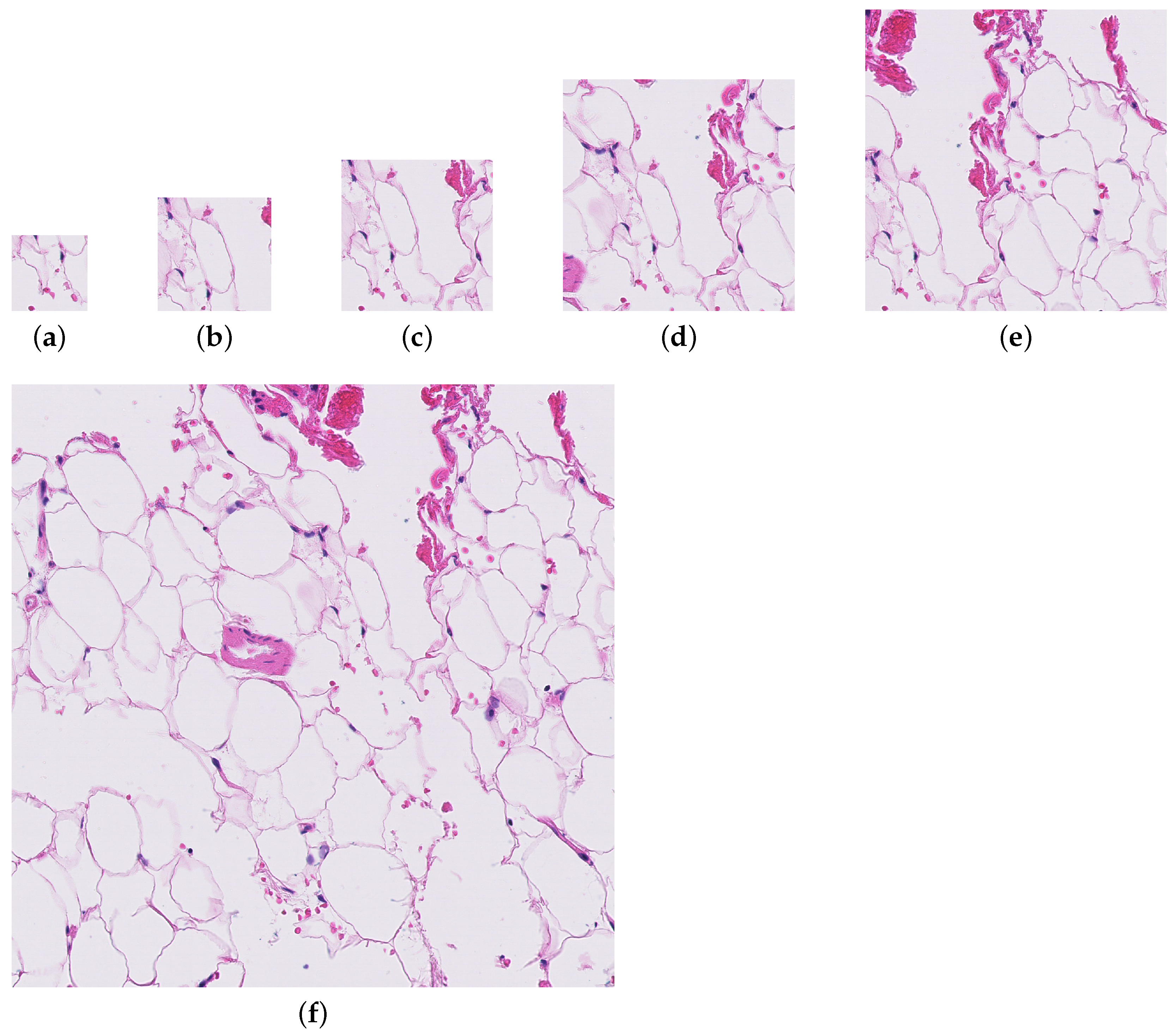
2.3.2. Comparison of Patch Sizes

In the reviewed related work, patch sizes range from 100 × 100 pixels to 1024 × 1024 pixels. Bándi et al. [18] reviewed submissions for the Camelyon17 challenge, which used a range of patch sizes between 256 × 256 pixels to 1920 × 1920 pixels both at level 0, and found that the smallest patch size provided enough context and is sufficient for analysis. A smaller patch size is beneficial if it provides enough information to the model, as, if a patch is too large, it will encounter the same computational problems that a WSI does. Conversely, some believe, such as Komura et al. [6] and Khened et al. [23], a larger patch size will result in better accuracy as smaller patches do not include sufficient context [23]. Similarly, Fell et al. [16] consulted with pathologists who noted that, for manual annotation, the typical patch size of 256 × 256 pixels would be too small and so larger patches may imitate the manual annotation process more closely. However, Deng et al. [15] found that small patches did not provide sufficient context for analysis, but large patches are too computationally expensive. Due to the lack of consensus on patch size, more work is needed to definitively find the optimal patch size.

2.4. Relevant Concepts and Technology

To ensure the reproducibility of WSI analysis methods and standardise the details included in research papers, a checklist of important details was created by Fell et al. [10]. This is a useful guideline for the implementation of the work and the related section of this article. It is important to note not all points are relevant to the work, specifically lesion and patient classification. The checklist is as follows [10]:

• The hardware and software platform the system was trained and tested on.
• The source of the data and how it can be accessed.
• How the data was split into train, validation, and testing sets.
• How or if the slides were normalised.
• How the background and any artefacts were removed from the slides.
• How patches were extracted from the image and any data augmentation that was applied.
• How the patches were labelled.
• How the patch classifier was trained, including technique, architecture, and hyper-parameters.
• How the slide classifier was trained, including pre-processing, technique, architecture, and hyper-parameters.
• How lesion detection was performed.
• How the patient classifier was trained, including, pre-processing, technique, architecture, and hyper-parameters.
• All metrics that are relevant to all the tasks.

Wang et al. [26], the winners of the Camelyon16 challenge evaluated four different deep-learning architectures for the analysis of WSIs: GoogLeNet, AlexNet, VGG16, and FaceNet. The patch classification stage was tested using these models and the accuracy of the classification was measured. The model that produced the best result, and the one used by Wang et al. for the final results of the analysis, was GoogLeNet which is a CNN based on the model created by the winners of ImageNet in 2014.

3. Proposed Methodology

3.1. Camelyon16 Winning Paper

The winning paper of the Camelyon16 challenge [26] was the main inspiration for the structure of the system. The Camelyon16 challenge is the source of the dataset used for the paper, which consists of a training set of 160 “normal” WSIs and 111 “tumour” WSIs and a testing set of 129 WSIs.

The overarching methodology of the winning paper is image pre-processing, patch-level classification, post-processing production of tumour probability heatmaps, and slide-level classification [26]. The image pre-processing stage involved only tissue segmentation to remove irrelevant white background from the WSIs and patch extraction. No colour standardisation or data augmentation was mentioned in the paper. Millions of patches of size 256 × 256 pixels were randomly extracted from training WSIs and used to train the model for patch-level classification. The patch-level classification stage results in a model that can predict if a patch contains any tumours. This model was then applied, in the post-processing stage, to overlapping patches extracted from a testing WSI, to produce a tumour probability heatmap corresponding to the image. Finally, features were extracted from the heatmaps which were then input into the slide-level classification model, a random forest classifier, to give a probability value for the presence of tumour in the WSI.

3.2. GoogLeNet

During the patch-level classification stage, Wang et al. [26] tested four different deep learning networks by evaluating the accuracy of the patch classification. The GoogLeNet network produced the best accuracy out of the four, with 98.4%. As the work uses similar methods and the same dataset, the GoogLeNet network was chosen to be the patch-level classification model architecture. GoogLeNet is a pretrained 22-layer deep convolutional neural network with a minimum image input size of 224 × 224 pixels. The architecture of the network is shown in Figure 2.

3.3. System Structure

There are four distinguishable stages in the overall structure of the work: data pre-processing, patch-level classification, production of tumour probability heatmaps, and slide-level classification. These processes were all involved in producing the final artefact, an accurate patch-based WSI analysis method. However, due to the need to train the machine learning models, the structure of the system used to produce the final artefact differs from the structure of the final artefact itself. The differences between the systems can be seen in Figure 3.

Figure 3a shows the process of producing the final artefact. This system first applies pre-processing to the WSIs from the training dataset to retrieve many normal and tumour patches. These patches are then used to train the patch classification model. The WSIs from the testing dataset are then split into patches and, for each WSI, a heatmap is created to represent the probability of each patch being tumourous, predicted from the previously trained patch classification model. The slide-level classification is then trained using a training subset of the heatmaps from which features are extracted.

Figure 3b represents the final artefact. This allows an unseen WSI to be split into patches, which are then input directly to the post-processing step to produce a tumour probability heatmap corresponding to the WSI. This heatmap is then input to the slide classification model, extracting the features of the heatmap to predict the probability that the slide is tumourous.

3.4. Camelyon16 Dataset

The dataset used for the work was the Grand Challenge Camelyon16 dataset of sentinel lymph node WSIs. This data is freely available to download from the Camelyon16 webpage [29].

The data is split into two folders, training and testing. The training folder contains the WSIs as .tif files and the lesion annotations as .xml files. There are 160 normal WSIs and 111 tumour WSIs for training, and the lesion annotations contain the coordinates of the tumours in each corresponding tumour WSI. The testing folder contains the WSIs as .tif files, the lesion annotations as .xml files, and a reference file. There are 129 WSIs to be used for testing, with the reference file containing the details for each file: the label i.e., normal or tumour, and the type of tumour. There is a lesion annotation file for each WSI in the test set that is labelled tumour. Figure 4 shows an example of a normal slide and a tumour slide.

The WSI is stored at multiple different resolution/magnification levels, shown by Figure 5. The images at different levels can be accessed separately to retrieve the WSI at the desired resolution. For this work, the WSIs are all retrieved at the highest resolution level, therefore containing the largest number of pixels possible. This is with the exception of the downsampling method where the aim is to use images of lower resolution.

3.5. OpenSlide

The WSI .tif files contain multiple versions of the slide image, at different resolutions. These are stored in a pyramid-like structure which cannot be accessed unless using a specialised library [29]. The OpenSlide library is a C library that can read WSIs, the Python binding of the library also includes a Deep Zoom generator. For the work, this library was chosen as it has functions to read WSIs, get the dimensions of each level of the WSI, and fetch regions of the WSI at a specified level. The additional Deep Zoom generator also provides the ability to split the OpenSlide object into tiles of a given size which is ideal for the aim of this work.

3.6. Pre-Processing

There are four main pre-processing steps for WSI analysis: tissue segmentation, colour normalisation, patch extraction, and data augmentation. For this work, only two of these pre-processing steps, tissue segmentation and patch extraction, were implemented. The decision to not perform colour normalisation was influenced by the Camelyon16 winning paper [26], which used the same dataset as used for this work. As colour normalisation is usually performed to remove stain variation within the dataset, and Wang et al. [26] did not apply colour normalisation, it was decided not to perform any kind of colour normalisation. Data augmentation was not deemed necessary as it is possible to extract hundreds of thousands of patches from each image in the dataset. These patches can be used to form a large training dataset, therefore eliminating the risk of overfitting due to lack of training data.

The aim of the tissue segmentation stage is to remove any unnecessary areas from the WSIs. For this paper, this step is focused on removing the background of the images. As can be seen in Figure 6, a WSI can consist of majority background which is not useful for the classification model. Without this pre-processing step, many of the patches extracted from the image may be background and therefore the model would be largely trained on irrelevant data and predict non-background patches poorly. This would also lead to a great deal of unnecessary computational time and power spent training the model, as a larger number of patches per image, and therefore a larger training dataset, would be required to achieve accurate predictions.

As the aim of the work is to implement a patch-based WSI analysis method, patch extraction is an essential pre-processing step. For this step, the entire WSIs are first split into patches. Most WSIs produce hundreds of thousands of patches per image, depending on the size which is specified when splitting up the WSI. The effect of using different patch sizes in this step will be investigated later in this report. The patches can also be overlapping by a specified number of pixels, which can provide some additional context to the patches to reduce the loss of spatial information.

The second part of patch extraction is to create a subset of patches from the entire set of patches, depending on the task. For the post-processing step using WSIs from test data, the entire patch dataset is used. However, to train the patch classification model, only a sample of patches from each WSI in the training dataset is used. There are multiple methods that can be used in patch extraction to choose a sample of patches from an image. In this paper, two of these methods, random sampling and informed sampling, are implemented and tested with the varied patch sizes.

For this work, there were two main pre-processing steps implemented: tissue segmentation (background removal) and patch extraction. The background removal pre-processing was implemented as part of the patch extraction pre-processing. The pre-processing stage results in the creation of a new dataset of patches and their labels, to be used as input to the patch-level classification model.

The pre-processing stage begins with the splitting of WSIs into all possible patches using a provided patch size. The total number of patches that this process results in varies as the WSIs have different dimensions. To retrieve a subset of patches for the training dataset, a sampling method must be used. The implementation of two sampling methods used for this work, random sampling and informed sampling, are described in Section 3.6.2 and Section 3.6.3. A Patch class object is created for each of the patches in the subset which performs functions including label retrieval, background check, and transformations.

The label retrieval for a patch is dependent on the slide label. For the training data, the slide label is contained within the filename, either “normal” or “tumour”. If a WSI has the “normal” slide label, all patches extracted from the WSI are labelled “normal” too. However, for slides labelled “tumour”, the patch label must be inferred from the lesion annotations. The lesion annotations are contained in .xml files via the coordinates of the tumour regions in a slide. These coordinates were collated into tumour regions by creating polygon objects for each tumour and saving each in a list of tumours for the corresponding slide. Figure 7 shows an example of the polygons representing tumours in a WSI graphed. To check if a patch contains tumour, the centre of the patch was found and used to create a point object. The list of polygons representing tumours was then looped through, and each one checked if it contained the centre of the patch. If the patch was deemed to be within a tumour, it was labelled “tumour”, if not it was labelled “normal”.

The “normal” and “tumour” labels for the patches were encoded using one hot encoding, with two values, the first representing the “normal” class and the second representing the “tumour” class. Therefore, a “normal” patch label contains a 1.0 in the first position and a 0.0 in the second position, and a “tumour” patch label has a 0.0 in the first position and a 1.0 in the second position.

3.6.1. Background Removal

The background removal step occurs when the patches are fetched in the sampling method. A background check was implemented by calculating the mean of the pixel values in the patch. If this mean is greater than a threshold, the patch is discarded and not added to the new training dataset. The threshold was determined with the aim of excluding as many background patches as possible without removing any tissue regions. This was achieved by comparison of example WSIs and corresponding images showing the pixels that would be discarded at the threshold. An image with all white pixels would have a mean pixel value of 256. However, to account for the slight off-white colour of the background of WSIs and general artefact, it was determined that any threshold above 240 would not remove significant background region. Therefore, a threshold of 240 was initially tested. However, this resulted in not all background region being removed, and in some cases none at all, so the threshold 230 was also tested and compared with 240. An example of this comparison is shown in Figure 8 and Figure 9. Ultimately, a threshold of 230 was chosen for the background segmentation as this removed significantly more irrelevant patches for many WSIs, yet still kept all relevant information. This threshold is independent of patch size, its value being ultimately driven by image content, rather than size, and the staining protocol, that is the contrast between tissue and background, etc. An alternative approach would have been to employ some type of colour normalization prior to thresholding [24] which we decided not to do so as to avoid introducing a potential confound into our analysis though it should be noted that the most recent findings in this realm suggest that colour normalization becomes unnecessary if a sufficient feature extractor is used [30].

3.6.2. Random Sampling Method

The random sampling method involves choosing, at random, a given number of patches from all the possible patches for an image. This random selection is done without replacement to avoid duplicates in the training data. Random sampling is a simple sampling method, but it can result in a significantly large class imbalance. When randomly sampling from a normal slide, all patches will be “normal”, either normal tissue or non-tissue regions. However, when sampling from a tumour slide, some patches will be tumour, but a large number are still “normal” patches. This means that the resulting dataset contains a much larger number of normal patches compared to tumour patches.

The random sampling method retrieves a subset of patches chosen at random. This was implemented by, for each WSI, iteratively fetching random patch addresses from the set of patches for the image and adding the corresponding patch to the training dataset. There is a defined maximum number of patches per image for the sampling method. The iterative process will continue until this maximum is reached or all patches have been fetched.

3.6.3. Informed Sampling Method

The informed sampling method counteracts the issue of class imbalance from the random sampling method. This method is more complex than random sampling as it uses the location of tumours in the slides. Normal slides are processed in the same way as in random sampling; a given number of patches are chosen randomly, all of which are “normal”. However, for tumour slides, the patches are sampled based on the location of the tumours in the slides. A given number of tumour-labelled patches are extracted in addition to the usual “normal” patches which are still chosen from the tumour slides. By specifying a similar value for the number of both the tumour and normal patches, a more balanced dataset can be produced, ensuring a reasonable proportion of the training dataset is tumour.

The informed sampling method creates a more balanced dataset than the random sampling method. This method was implemented similarly to the random sampling, except, for tumour slides, the maximum number of patches is split into a maximum number for normal patches and a maximum number for tumour patches. The two maximum values for the tumour slides are chosen to be equal and the sum of them is equal to the maximum number of patches for the normal slides. The tumour patches are sampled from a list of patches in tumour regions fetched from the lesion annotation files. The resulting dataset remains slightly unbalanced, although to a much lesser degree. It is not possible to completely balance the dataset without using a small number of patches per image as there is significantly fewer tumour patches compared to normal patches.

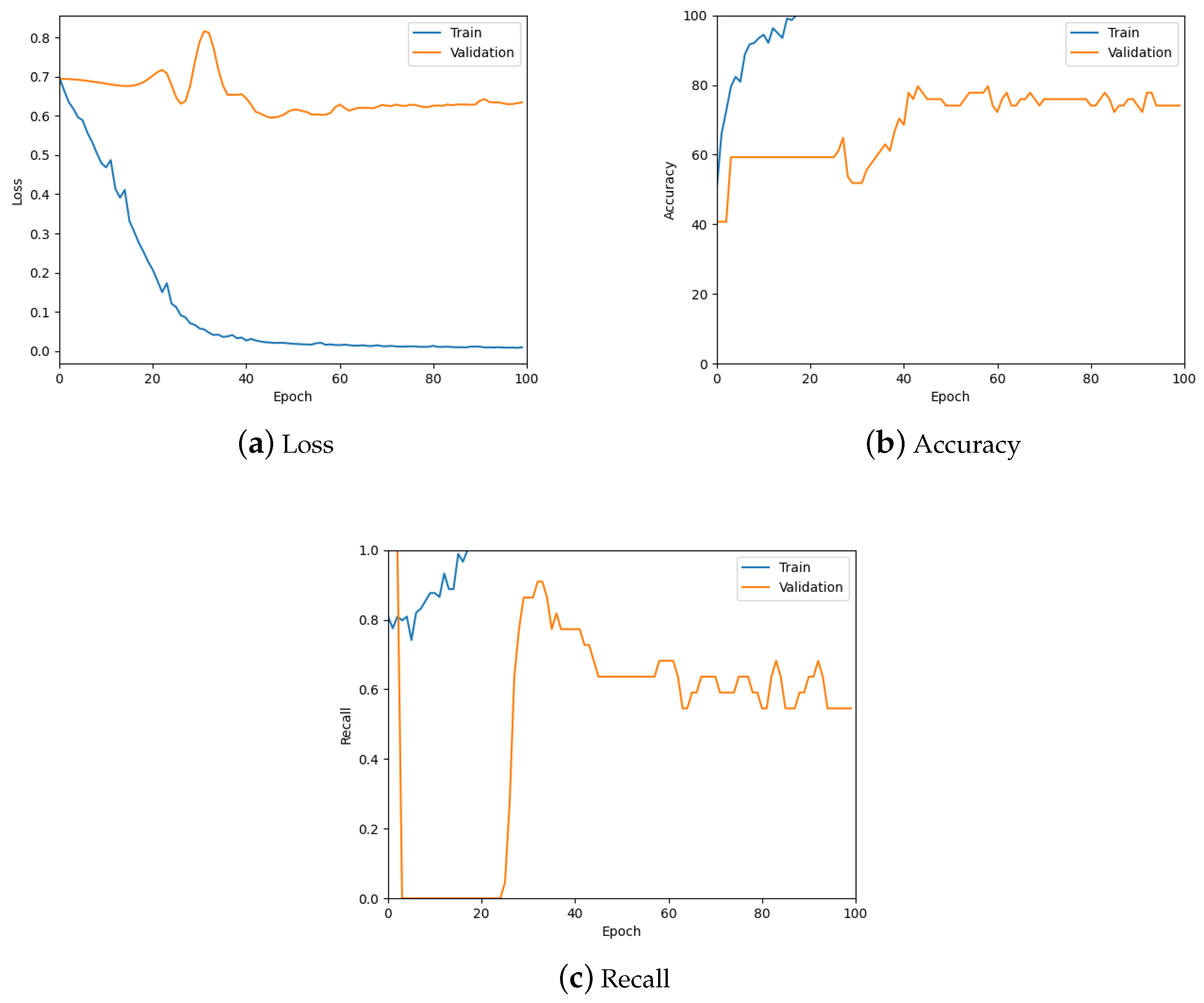
3.7. Patch-Level Classification

The aim of the patch-level classification model is to predict the probability of a patch containing tumourous tissue. This model takes as input the pre-processed patches sampled from the training data. It outputs a probability value for both the normal class and the tumour class. The model is trained and optimised based only on the accuracy of the patch-level classification. The patch classification is the foundation of the remainder of the system, therefore it is essential that the model performs well.

As this stage focuses on performing patch-level classifications, rather than slide-level or lesion-level, the input patches are independent from their original WSIs. Therefore, the model learns only from the features and morphological information given by a patch individually. This also means there is no spatial information provided to the model which is the most significant drawback of patch-based analysis methods.

The patch-level classification stage focuses on the prediction of patch-level labels by training a neural network. This step was implemented using the GoogLeNet architecture described in Section 3.2 which was loaded from PyTorch in the PatchAnalysis script. As this network usually has 1000 output nodes, the number of classes for this problem, two, normal and tumour, was specified when loading the model.

The input data for the model originates from the pre-processing step. A custom dataset was created to take the directory of the patch files and create a dataset consisting of a list of the patch filenames and a list of the patch labels. The __getitem__ function of the dataset class then fetches the patch, as a tensor, from the file at the given index, alongside the label for the patch. To train and evaluate the model, the patch dataset was split into train and validation datasets using a stratified split based on the patch labels to ensure the tumour patches were evenly distributed between the datasets. The size of the validation dataset was specified to be 20% of the original dataset. All testing was performed using a separate test corpus provided as part of the challenge data set.

The version of WSI analysis performed in this work is a binary classification problem. However, as the GoogLeNet network has been used, which requires a minimum of two classes, the binary classification is implemented using one hot encoding with a class representing “normal” and a class representing “tumour”. Therefore, despite this being a binary problem, the loss function, optimiser, and activation function were chosen based on the model architecture having two output nodes. Categorical cross entropy loss was chosen for the loss function as this is commonly used in classification problems with success; binary cross entropy loss was not possible to use given the one hot encoded outputs. The Adam optimiser was used due to its ability to adapt well to increase speed and accuracy of the predictions. The softmax activation function was used to convert the model outputs to probabilities. This was chosen over the sigmoid function as the classes are mutually exclusive and the probabilities output from the softmax function sum to one.

3.7.1. Testing

The patch classification model was tested using the validation set, the confusion matrix for which can be seen in

Table 1. Confusion matrix for the patch classification model on the validation set.

		Actual
		Positive	Negative
Predicted	Positive	201	0
	Negative	163	7798

, and by analysing the graphs for the loss, accuracy and recall of the predictions to ensure the model was learning properly. Figure 10 shows these graphs for the trained model with a patch size of 256; also see the summary in

Table 2. The loss, accuracy, and recall values used for testing the patch classification model. To account for stochastic fluctuations all values are reported for the exact epoch noted, followed by the average of the values corresponding to epochs in a window centred at the said epoch.

		Epoch
		25	50	75	100
Train	Accuracy (%)	98.72/98.24	99.34/99.24	99.23/98.82	99.44/99.81
	Recall	0.99/0.99	1.0/0.99	1.0/0.99	1.0/1.0
	Loss	0.04/0.04	0.01/0.02	0.01/0.02	0.01/0.01
Validation	Accuracy (%)	90.03/94.94	99.03/98.72	99.03/98.72	98.83/98.93
	Recall	0.80/0.73	0.63/0.69	0.48/0.54	0.55/0.56
	Loss	0.67/0.67	0.83/0.67	1.37/1.13	0.95/1.12

. From these, it is possible to see the model is predicting well overall and there is low loss. However, there is some overfitting, specifically for the tumour class as can be seen in Figure 10c, which was addressed during hyper-parameter testing.

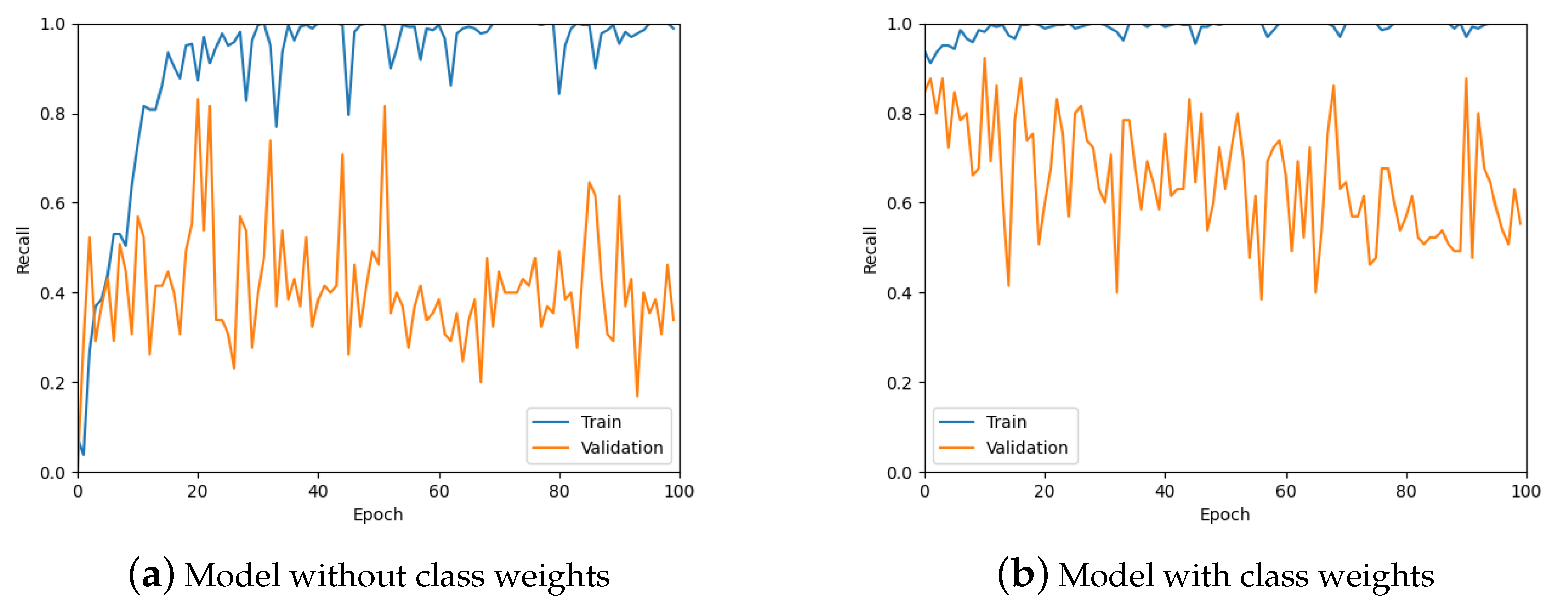
3.7.2. Hyper-Parameter Tuning

The hyper-parameters that were tuned for this model were learning rate, class weights, patches extracted per image and number of epochs. These parameters were evaluated using the loss, accuracy, and recall measures for the model’s predictions. All hyper-parameter tuning was performed on a patch dataset with 100 patches of size 256 × 256 per WSI, sampled using the random sampling method. Except where otherwise specified, the hyper-parameters were kept the same for all patch size and sampling method tests.

The learning rate was optimised by testing values on a log scale, from ${10}^{-1}$ to ${10}^{-5}$, and comparing the loss, accuracy, and recall on the validation set. The results of these measurements are shown in Figure 11 (also see

Table 3. The validation loss, accuracy, and recall values for a range of learning rates used to find the best hyper-parameter value. To account for stochastic fluctuations all values are reported for the exact epoch noted, followed by the average of the values corresponding to epochs in a window centred at the said epoch.

		Epoch
Learning Rate		25	50	75	100
${10}^{-5}$	Accuracy (%)	98.67/98.67	99.11/99.11	99.20/99.20	99.20/99.20
	Recall	0.18/0.30	0.47/0.41	0.37/0.43	0.33/0.31
	Loss	0.06/0.05	0.05/0.05	0.06/0.05	0.09/0.08
${10}^{-4}$	Accuracy (%)	99.11/99.11	99.20/99.20	99.38/99.28	99.11/99.11
	Recall	0.31/0.35	0.49/0.47	0.43/0.41	0.32/0.28
	Loss	0.08/0.07	0.06/0.06	0.07/0.07	0.09/0.11
0.001	Accuracy (%)	98.32/98.67	99.56/99.56	99.38/99.38	99.38/99.38
	Recall	0.77/0.61	0.33/0.40	0.51/0.49	0.42/0.42
	Loss	0.07/0.06	0.08/0.07	0.07/0.07	0.13/0.13
0.01	Accuracy (%)	99.38/99.38	98.94/98.58	99.47/99.47	99.38/99.38
	Recall	0.52/0.39	0.43/0.64	0.23/0.43	0.23/0.40
	Loss	0.06/0.07	0.04/0.05	0.12/0.08	0.10/0.09
0.1	Accuracy (%)	99.03/99.03	99.20/99.20	99.03/99.03	99.03/99.03
	Recall	0.00/0.00	0.32/0.30	0.00/0.00	0.00/0.00
	Loss	0.07/0.05	0.04/0.04	0.05/0.04	0.04/0.04

). From the accuracy graph, it is evident that the learning rate affects this metric very little, particularly by the end of the 100 epochs. Therefore, the final learning rate was chosen based on loss and recall measurements. From the loss, ${10}^{-1}$ appears to be the best choice, but also gives the lowest recall value. Consequently, a learning rate of ${10}^{-5}$ was chosen which also has low loss but gives a similar recall to other learning rates.

From Figure 11, it is clear that the recall values are not ideal given that the aim of the work is to detect tumours. Therefore, class weights were added to the loss function in an attempt to improve the recall of the predictions. A comparison of class weights versus no class weights can be seen in Figure 12. It is obvious from these graphs that using class weights is much more optimal for this work.

Another hyper-parameter that was investigated is the number of patches sampled per image. The results of this investigation are shown in Figure 13 which shows the validation loss, accuracy, and recall for 10, 25, 50, 100, and 150 patches per image; a further summary can be found in

Table 4. The loss, accuracy, and recall for the model using various numbers of patches per WSI in the training set. To account for stochastic fluctuations all values are reported for the exact epoch noted, followed by the average of the values corresponding to epochs in a window centred at the said epoch.

		Epoch
No. Patches		25	50	75	100
10	Accuracy (%)	98.23/98.32	99.03/99.03	94.06/94.62	99.03/99.03
	Recall	0.33/0.5	0.17/0.17	0.84/0.89	0.33/0.27
	Loss	0.76/0.48	1.26/1.38	0.22/0.22	1.27/1.28
25	Accuracy (%)	97.96/98.32	94.42/94.83	88.74/88.74	98.85/98.96
	Recall	0.51/0.51	0.73/0.73	0.81/0.85	0.47/0.60
	Loss	0.66/0.69	0.36/0.40	0.37/0.41	0.85/0.67
50	Accuracy (%)	92.11/95.83	99.03/98.97	98.85/99.14	98.67/98.75
	Recall	0.88/0.78	0.53/0.59	0.64/0.64	0.62/0.60
	Loss	0.32/0.39	5.26/2.22	0.70/0.72	0.84/0.80
100	Accuracy (%)	96.19/97.96	99.03/98.29	98.85/94.71	98.49/98.49
	Recall	0.77/0.64	0.45/0.64	0.62/0.70	0.71/0.64
	Loss	0.38/0.70	1.17/0.84	1.07/0.95	0.84/0.85
150	Accuracy (%)	98.67/94.42	99.03/99.16	98.85/99.14	99.56/99.26
	Recall	0.81/0.83	0.65/0.68	0.70/0.71	0.64/0.62
	Loss	0.57/0.63	0.92/0.98	0.89/0.88	1.37/1.39

. Many of the values are similar for the various numbers of patches. However, the largest number of patches per image gave the most stable values. Therefore, 150 patches were sampled from each image for the remainder of the work with the exception of the 1024 × 1024 patch size, which only had 50 samples from each image due to the large patch size.

As can be seen from previous hyper-parameter tuning, the maximum epoch value that was previously used is sufficient for training the model. The accuracy has plateaued and, based on recall graphs, the model is beginning to overfit for the tumour data. The trained model used for the production of heatmaps is selected individually for each classification using the loss, accuracy, and recall graphs to choose the best performing model.

The batch size used varied depending on the patch size as increasing the patch size led to issues with the CUDA memory so a decrease in batch size was required to run the patch classification.

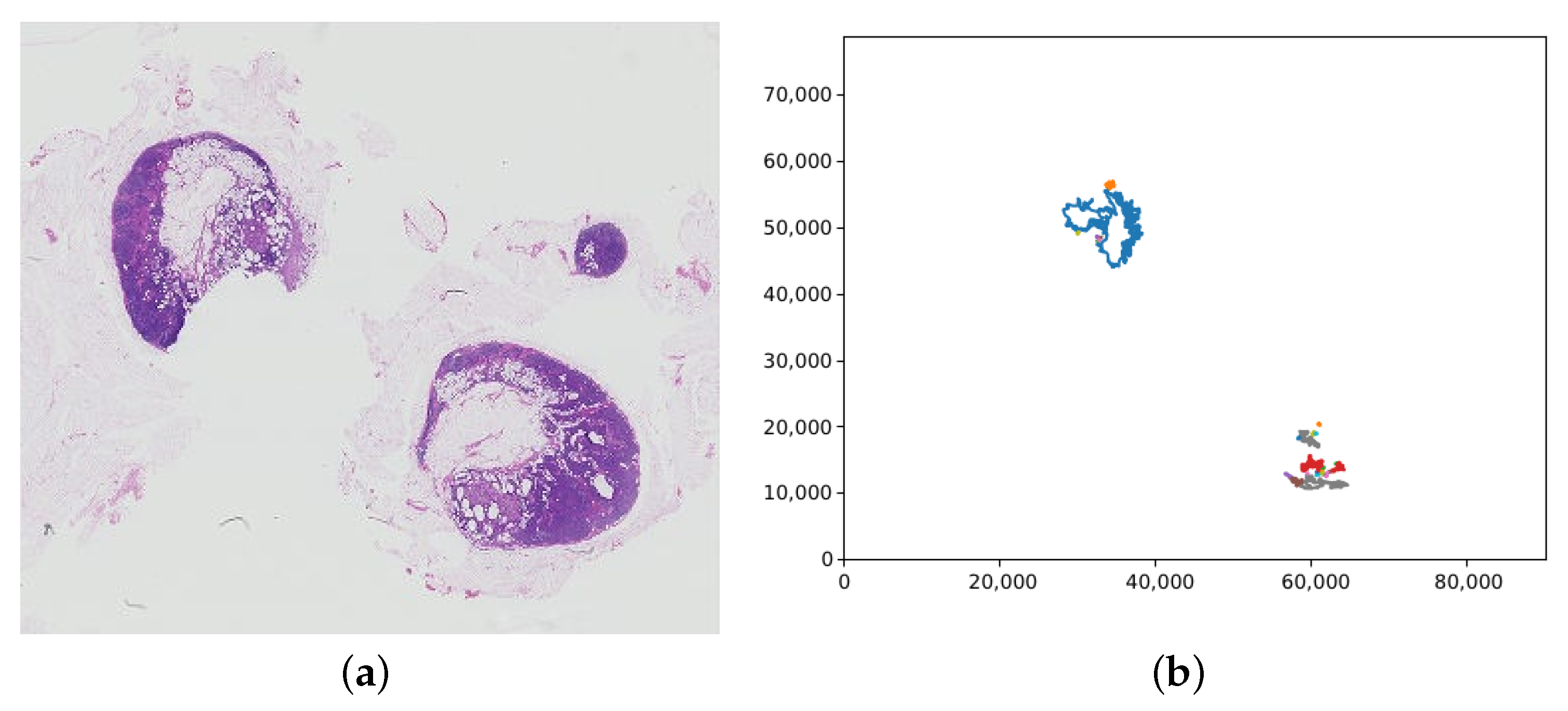
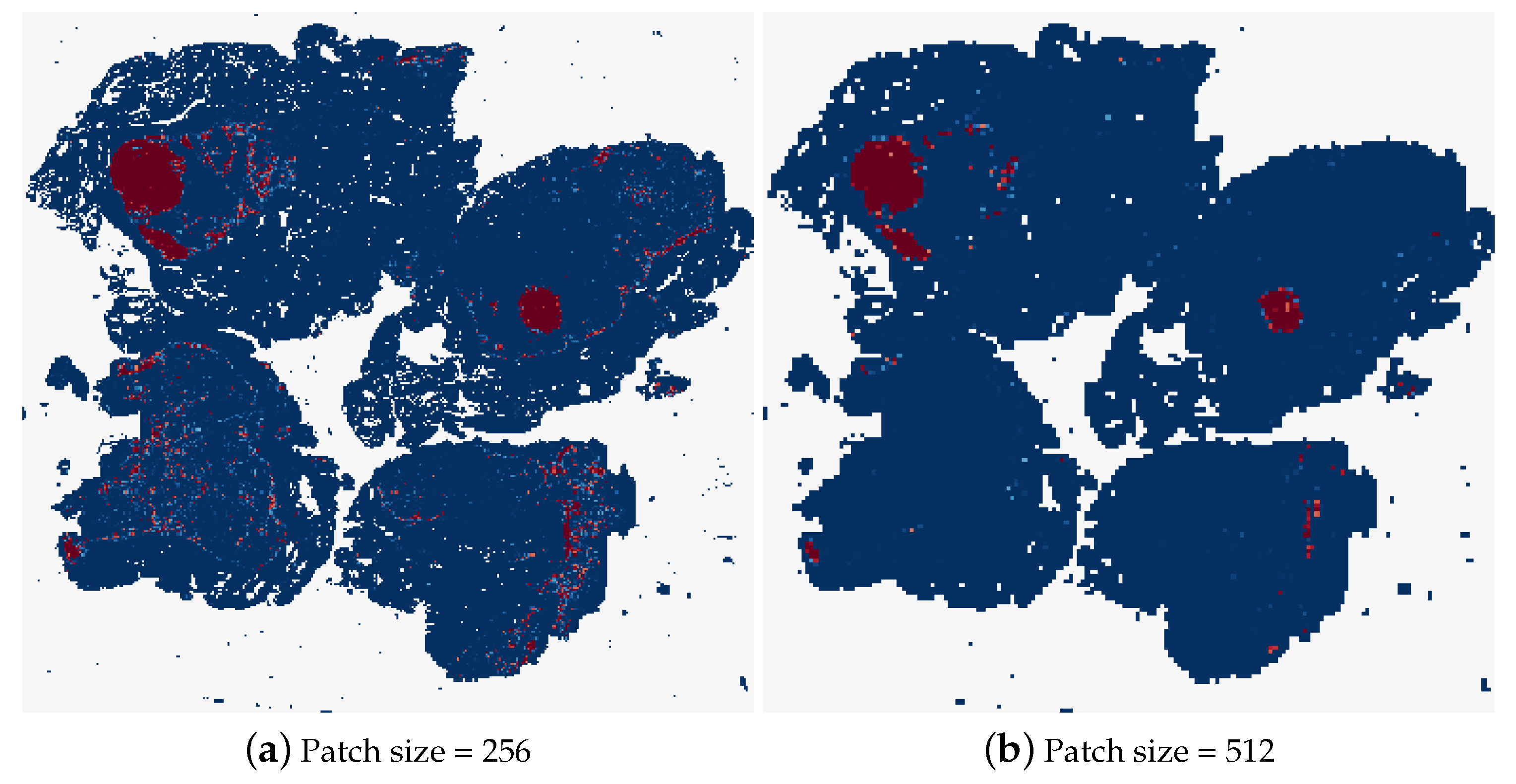
3.8. Production of Tumour Probability Map

This stage of the system creates heatmaps that correspond to each WSI in the testing dataset. The testing data, one WSI at a time, undergoes patch extraction resulting in a set of all patches from a WSI. The trained patch-level classification model is applied to this set of patches and predicts, for each patch, the probability that the patch contains tumourous tissue. The tumour probabilities are then displayed in a heatmap. From the heatmaps, it is possible to see the correlation between areas of high tumour probability and the location of tumours in the corresponding WSI. Therefore, if a test WSI is classified as tumour, these heatmaps can be used to retrieve the location of tumours in the WSI for further analysis by a pathologist.

The production of the tumour probability heatmaps is a post-processing step which involves applying the trained model from the previous stage, rather than being a model itself. The heatmaps produced are split into training and testing data. The training heatmaps become the input for the second model of the system, and the testing data is used to test the accuracy of the model and the overall patch-based WSI analysis method.

The production of the tumour probability map from a WSI can be split into two parts, both of which are implemented in the CreateHeatmap script. The first part involves splitting the WSI into patches and the second part uses the trained patch-level classification model to get the predictions for the patches which form the heatmap.

The model is loaded from a file of the saved trained model produced by the previous step of the process. The WSI is then loaded and split into patches using the Deep Zoom generator. The columns and rows that formulate the addresses of the patches are iterated through and each patch address is added to a list, provided it is not part of the background of the slide. A custom dataset, AllPatchDataset, is then used to create a dataset with these patch addresses and the generator. The __getitem__ function in this dataset fetches the patch at the address given by the index and preprocesses it before returning the patch.

The heatmap data begins as an array of zeros with the dimensions of the number of columns and rows. This ensures that any background patches that are not in the dataset are automatically given a value of 0 for the heatmap. For each patch in the dataset, the probability predictions for the two classes are produced by the trained model. The probability values for the “normal” class are negated to give values between −1 and 0. The “tumour” class predictions are untouched. The highest absolute value between the predictions for each patch is added to the heatmap data in the position given by the column and row of the address of the patch.

Once the whole dataset has been predicted, the heatmap data is plotted using the seaborn package and the resulting heatmap is saved as an image into a directory of heatmaps. Every heatmap is plotted with the same minimum and maximum values to ensure the colour scale is equal for the next stage of feature extraction and training. A file containing a list of the probability values is also saved to aid in feature extraction in the next stage.

Each heatmap is saved with the label of the slide in the filename to be used for the slide classification. The label for each test WSI is contained within the reference.csv file from the dataset. This file is read using pandas and, for each WSI, the corresponding label is fetched from the dataset and added to the heatmap’s filename.

Testing

This post-processing stage was tested by inspecting the resulting heatmaps. The heatmaps corresponding to both normal and tumour WSIs were compared to check that the heatmap creation was successful. Different colour maps and formats were also tested to identify the optimal parameters for the heatmaps. Figure 14 shows an alternative colour map that was tested prior to deciding to show normal probabilities in addition to tumour probabilities. This figure also shows a heatmap that only uses classification results rather than probabilities. Using the classification results did not provide the information required for the feature extraction that is required for slide classification.

The final style of heatmaps, including colour map, is shown in Figure 15. These heatmaps were created using the reversed “BuRd” colour map with the scale of probabilities being between −1 and 1. The regions that are saturations of blue are values between −1 and 0, normal tissue, and the regions that are saturations of red are between 0 and 1, tumour tissue.

3.9. Slide-Level Classification

The slide-level classification model is the final step in the classification of WSIs. This model is trained using features extracted from each of the tumour probability heatmaps, for example, the percentage of the slide that is tumour, the average probability values, and the frequency of high probability tumour areas. These features are input to the model alongside the labels for the corresponding WSIs.

The trained model is tested using extracted features from the heatmaps in the testing data. The metrics resulting from this testing are used to evaluate the accuracy of the entire WSI analysis. These measures will be used to evaluate and compare the various patch sizes and methods used in this work.

The slide-level classification task is the last in the analysis of WSIs. The aim of this classification is to predict the slide-level label for a WSI from the corresponding heatmap produced in the previous step. This is implemented with a random forest architecture, using the sci-kit learn package.

The dataset for the input of the model is the heatmap data. However, as this dataset consists of images of various sizes, the pre-processing step, feature extraction, must first be undertaken. Feature extraction is performed to collect features of the images and data, as numerical values, that can be input into the classifier. The feature extraction process is detailed in Section 3.9.1. This step is performed within a custom dataset class, HeatmapDataset. This class takes the path of the heatmap directory, extracts features from each of the images in the directory, and gets the label for the instance. The input data was split into training and test sets using a stratified split with a test set size of 0.2. A validation set was not necessary for this model as no hyper-parameter tuning was performed.

The output for this classification is the final classification result for the analysis of the WSI. The labels for the slides are one-hot encoded, in the same way as done for the patch-level classification model. Therefore, the output produced by the model, for each input, is either $[1.0,0.0]$ for “normal” or $[0.0,1.0]$ for “tumour”.

3.9.1. Feature Extraction

Feature extraction is necessary for this model as the input images, the heatmaps, are of varying sizes. It is not possible to resize these images to make a dataset of images of the same dimensions as this would warp the information provided by the heatmap. A feature extraction process was implemented that extracts 22 statistical and mophological features from each heatmap image and corresponding probabilities. In choosing these features, inspiration was taken from both the Camelyon16 winning paper [26] and from Fu et al. who investigated tumour detection in whole slide images [31].

The first feature extracted is the percentage of tissue that is predicted to be tumour. This was implemented by getting the sum of positive probabilities, the tumour patches, and the sum of negative probabilities, the normal patches. The percentage of tumour patches over the entire tissue region, tumour and normal patches, was then calculated.

The next features are the number of tumour regions and the size of the largest tumour region in the heatmap. This is implemented by extracting a mask of the tumour regions. The number of tumour regions found in this mask is the first of these features. Then the largest continuous area of tumour patches is found and the size calculated in pixels. Figure 16 shows an example of the mask of the tumour regions in a WSI.

The remaining extracted features are based on the statistics of the probabilities. The probability values are split into positive (tumour) probabilities and negative (normal) probabilities. The absolute value of each of the negative probabilities was taken for ease in calculations. From both of these sets of probabilities, nine values were calculated from the data. These values were the mean, median, mode, variance, standard deviation, minimum, maximum, range, and sum.

Other features were extracted to test for effectiveness, such as the class with the largest mean and the class with the largest number of patches. However, both of these values were largely the same for all slides, whether normal or tumour, and so were deemed not useful to the classifier.

3.9.2. Testing

This stage was tested using two methods. The feature extraction tasks were tested by printing out the features for various heatmap instances and analysing the values to ensure they appeared reasonable. The classifier was tested by analysing the accuracy, recall, and AUC measurements for the predictions to check that the predictions given were reasonable.

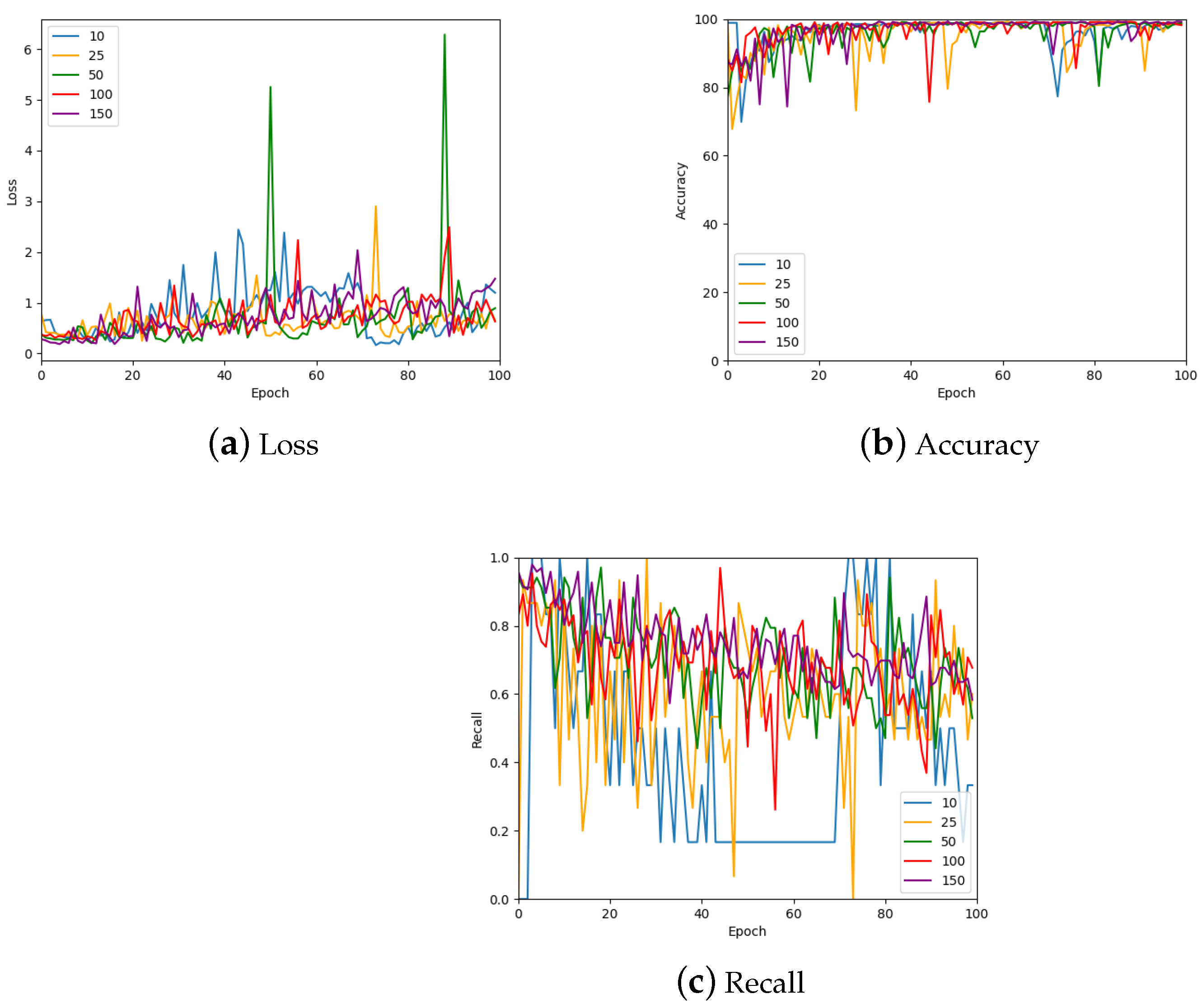
3.10. Testing the Effects of Patch Size

Using the final structure of the work, various patch sizes were tested. The entire process of patch dataset creation, patch classification, heatmap creation, and finally slide classification was performed for each patch size. The results of these tests are detailed in Section 4.1.

3.11. Downsampling Analysis Method

Downsampling is an alternative method used to counteract the problems faced when analysing WSIs. This can be used alone or in conjunction with patch extraction. As the original size of a WSI file is too large, downsampling reduces the resolution of the image, by a downsampling factor, therefore reducing the size of the image.

If the downsampling factor is large enough, the resulting downsampled image can be input directly into a model to predict the probability of tumour. This removes the need for splitting the image into patches and can be performed using only one model to predict the slide-level classification. Another option is using a combination of downsampling and patch extraction. An image can be moderately downsampled and then patch extraction can be performed on the downsampled image.

In general, patch-based methods are preferred over downsampling methods. When the resolution of a WSI is reduced, a significant amount of morphological information and fine detail can be lost. This can have a detrimental effect on the accuracy of the model and make the resulting model unusable in genuine clinical scenarios.

The downsampling-based WSI method involves inputting downsampled WSIs into a model for classification. This does not entail any patch extraction or related steps. The model used for this method was the GoogLeNet network, as used in the patch-level classification. As in the patch-level classification, the labels for the slides were one hot encoded to provide a two output node model as required by the GoogLeNet network.

This method was implemented by first creating a new dataset of the WSIs at the lowest resolution possible, from the training and testing WSIs. For the training of the model, the dataset of downsampled training WSIs was then split into training and validation sets using a stratified split with a validation set size of 0.2. For the testing and evaluation of the trained model, the set of downsampled testing WSIs was used.

Pre-processing for this method involved downsampling the images, resizing the images to 256 × 256, transforming to tensors, and normalisation. The downsampling occurs in the creation of the new dataset, prior to any analysis. When getting the items in the dataset with the dataloader, the remaining pre-processing steps are applied to the images. The resizing of the images is far from ideal as some are resized more significantly than others and so are not very comparable. However, this is necessary as the GoogLeNet network only accepts datasets of images of equal sizes. The transformation to tensor and normalisation is also required by the network.

The same loss function, optimiser, learning rate, and activation function as the patch classification model were used given the use of the same network and input image size. A few learning rates were tested but this appeared to have little effect on the accuracy of the model.

The final analysis of the WSIs was implemented by loading the best trained model and inputting the downsampled test WSIs. The predictions produced were evaluated using the accuracy and recall metrics.

Testing

This model was tested similarly to the patch-level classification model, using the loss, accuracy, and recall graphs. Figure 17 contains the corresponding three graphs (also see the summary in see

Table 5. The loss, accuracy, and recall values used for testing the downsampled slide classification model. To account for stochastic fluctuations all values are reported for the exact epoch noted, followed by the average of the values corresponding to epochs in a window centred at the said epoch.

		Epoch
		25	50	75	100
Train	Accuracy (%)	100.00/100.00	100.00/100.00	100.00/100.00	100.00/100.00
	Recall	1.0/1.0	1.0/1.0	1.0/1.0	1.0/1.0
	Loss	0.11/0.11	0.02/0.02	0.01/0.01	0.01/0.01
Validation	Accuracy (%)	59.35/60.00	74.26/74.26	76.04/76.04	74.26/74.26
	Recall	0.04/0.13	0.64/0.64	0.64/0.62	0.55/0.55
	Loss	0.65/0.65	0.62/0.62	0.63/0.63	0.63/0.63

) where it can be observed that the model is predicting the slide label well.

3.12. Metrics

The metrics used for the evaluation of the models are dependent on the task. There were three sets of metrics used throughout the work, which consisted of some combination of the loss, accuracy, recall, and AUC measurements. The performance of the patch-level classification model was measured using loss, accuracy, and recall. The final slide-level classification for the patch-based method was evaluated with the accuracy, recall, and AUC metrics. For this model, AUC is included as this is the primary metric used to evaluate the model in the Camelyon16 winning paper [26]. In analysing the training, the downsampled slide classification model, loss, accuracy, and recall were used. The measures used for the slide classification model, using the downsampled method, were accuracy and recall.

The loss values used were calculated from the model’s direct output, prior to softmax, using the cross entropy loss function. For the patch-level classification model, the loss function was given class weights due to the unbalanced nature of the datasets produced by random sampling. Cross entropy loss is used when a model’s output is class probabilities. The calculated loss value will increase if the probabilities of the classes are getting further from the true values. The equation for calculating cross entropy loss is

$$H\left(x\right)=-\left(P\right(“\mathrm{normal}”)\ast log(Q\left(“\mathrm{normal}”\right)+P\left(“\mathrm{tumour}”\right)\ast log\left(Q\right(“\mathrm{tumour}”\left)\right)$$

where $P\left(x\right)$ is the true probability of x and $Q\left(x\right)$ is the predicted probability of x.

The accuracy of the model is essentially the percentage of correctly predicted labels. In all instances, the predicted label is calculated by taking the class with largest probability for each patch/slide. The equation for calculating the accuracy is

$$\mathrm{accuracy}=\mathrm{number}\mathrm{of}\mathrm{correct}\mathrm{predictions}/\mathrm{size}\mathrm{of}\mathrm{dataset}*100$$

Recall is a measure of the accuracy of only the positive class, the “tumour” class. A good recall is particularly important for the analysis of WSIs as the misclassification of a tumour slide could have dire consequences. The observation of recall values is also key for the randomly sampled datasets due to the significant class imbalance. The equation for calculating the recall is

$$\mathrm{recall}=\mathrm{number}\mathrm{of}\mathrm{correctly}\mathrm{predicted}“\mathrm{tumour}”/\mathrm{number}\mathrm{of}“\mathrm{tumour}”\mathrm{in}\mathrm{the}\mathrm{dataset}$$

The AUC measure is calculated for the slide-level classification to allow comparison between this model and related work as it is a commonly used metric in WSI analysis methods. AUC stands for area under the ROC (receiving operator characteristic) curve. This is calculated by taking the integral of the ROC curve.

For the patch-level classification, and both downsampling models, the accuracy and recall were calculated manually using these formulae. The slide-level classification used the scikit-learn metrics to get the accuracy, recall, and AUC.

4. Results and Evaluation

4.1. Results of the Effect of Patch Size

To investigate the effect of patch size, the patch-based WSI analysis method was performed using a variety of patch sizes with the final classification results recorded for evaluation. Although not formally evaluated, the patch-level classification accuracy was close to 100% for all patch sizes for both sampling methods. However, the informed sampling method gave higher recall values, 90–98%, for the patch sizes tested, compared to the corresponding patch sizes sampled using random sampling, 60–70%.

Different patch sizes for the random sampling method were tested first, the results of which can be found in

Table 6. Results for the random sampling method.

Patch Size (px)	Accuracy (%)	Recall	AUC
256	73	0.60	0.71
384	54	0.30	0.49
512	69	0.50	0.66
786	62	0.60	0.61

. The typical patch size used in related work is 256 × 256 pixels, therefore, this was the first patch size tested. It was not possible to decrease the patch size by a significant amount from here, as the GoogLeNet network requires inputs of at least 224 × 224 pixels. While patches with smaller dimensions than this could be resized to input to the model, this could skew the patch size evaluation. Therefore, it was decided to double the patch size and observe the effects, testing the patch-based method using 512 × 512 patches. As can be seen in Table 6, this patch size caused a decrease in the accuracy of the model, with the tumour slide classification only correct 50% of the time. Figure 18 shows the heatmaps corresponding to the same test image for these two patch sizes. It is clear that a lot of detail in the heatmap is lost by increasing the patch size. Although the heatmap using 512 pixel size patches contains less uncertain predictions, where the colour of the patch is not at either of the extremes, dark blue for normal and dark red for tumour.

As there was a decrease in the accuracy, the next patch size attempted was the mean of the previous two, 384 × 384. This was followed by testing 1.5 times the current largest patch size, giving a patch size of 786, to evaluate if the downward trend continued. Neither of these patch sizes yielded a model that proved to be as accurate as the first, 256 patch size, model. Testing with the 786 × 786 patch size shows that it continues the decrease that was observed between patch sizes 256 and 512 in two metrics, accuracy and AUC. However, the recall value for this model is higher than the 512 patch size and equal to the 256 patch size. Given the importance of the recall for this task, a patch size of 786 should be considered over patches of 512 × 512. Based on the results of the other patch sizes, the metrics for the 384 patch size test appear to be an anomaly given the significant decrease in all three measures. Extrapolating from the trend between the remaining three patch sizes, the random sampling method predicts best when used with a smaller patch size.

Given the trend observed for random sampling, increasing patch size leads to decrease in accuracy, the informed sampling method was evaluated next. This method was evaluated with two of the same patch sizes as the random sampling, 256 and 512, and one other, 1024. The smallest patch size, 256 was tested first as this proved to be the most successful for the random sampling method. Patches of size 512 × 512 were then tested to see if the same downward trend applies for this sampling method. This proved to be true, however, rather than try the same 1.5 times larger patch size as done in the random sampling method, it was decided to evaluate a more extreme patch size of 1024 × 1024. As can be seen in

Table 7. Results for the informed sampling method.

Patch Size (px)	Accuracy (%)	Recall	AUC
256	81	0.60	0.79
512	65	0.30	0.59
1024	58	0.70	0.60

, a decrease in accuracy occurred between patch sizes 512 and 1024. However, the largest patch size gave the highest recall value, similarly to the random sampling method, where the largest patch size gave the equal highest recall value. Despite the significance of the recall for this task, the large decrease in overall accuracy between 256 patch size and 1024 patch size is too severe to ignore in favour of the higher recall.

4.2. Comparison of Methods

For both the random sampling method and informed sampling method, the smallest patch size tested, 256 × 256, produced the most accurate slide-level predictions. The informed sampling method proved to be superior to the random sampling method for this patch size giving an accuracy of 81% compared to 73%. However, the other patch size tested with both sampling methods, 512 × 512, achieved better results using the random sampling method, with a significant difference in the recall values, 0.5 for random sampling and 0.3 for informed sampling.

Here we also note that all of the achieved levels of accuracy could be further increased by the employment of techniques such as hard negative mining following the standard training protocol, as a means of reducing false positive errors. Had this been done the ultimate performance would have been higher, benefiting both from this feedback loop and the optimal patch size. However since our goal was not to employs all means available so as to engineer the highest performing systems based on the evaluated architectures but rather to assess the impact of patch size specifically, we made no such efforts.

The patch-based method and downsampling method can also be compared. The best patch method gave an accuracy of 81% and a recall of 0.60. The downsampling method gave significantly lower values, with accuracy at 64% and recall 0.49. This is the expected result, given the loss of fine detail that occurs in the downsampling of WSIs. However, given the lack of investigation into the best downsampling factor, this may not be a fair comparison. It is possible, by finding the optimal downsampling factor, the downsampling method could prove to be as accurate as the patch-based method.

4.3. Related Work

The Camelyon16 winning paper [26] was used throughout the work as guidance for the methodology of the system. This paper did not investigate the effect of patch size but was focused on the optimisation of the accuracy of the WSI analysis model for the Camelyon16 challenge. The research produced a model with an AUC score of 0.925 using patches of size 256 × 256. This is significantly higher than the one achieved by this work, 0.79 for the optimal method. However, the aim of this work was focused on the effect of patch size and used significantly fewer patches for training compared, with Wang et al. using millions of normal and tumour patches compared to around 40,000 used for this work.

The most significant related work is the paper by Fell et al. [16] who also did an investigation into patch size, using a similar methodology to this work and the Camelyon16 winning paper [26]. Three patch sizes were tested, 256, 512, and 1024. Fell et al. found that the largest patch size, 1024, provided the best model for analysis of the WSIs. This is in contrast to the findings of this paper, although not entirely when considering the recall rather than the accuracy. With a patch size of 1024 × 1024 pixels, an accuracy of 90% was achieved, compared to 81% for this work, and a recall of 97%, compared to 60%. The model implemented by Fell et al. was evidently very successful in the analysis of WSIs. However, it is difficult to compare as a dataset of 2909 WSIs was used compared to the dataset of 271 training WSIs and 129 testing WSIs that was used for this work.

4.4. Conclusions

The work successfully implemented a patch-based WSI analysis method and evaluated the effect of patch size, giving an optimal method using a patch size of 256 × 256 sampled using the informed sampling method. Both a random sampling method and an informed sampling method, using tumour region location, were implemented allowing for thorough investigation into the patch sizes using these different methods. Based on the classification results, the more accurate of the two sampling methods is dependent on the patch size. However, the optimal patch size/sampling method pair used the informed sampling method. A basic downsampling method was also tested, allowing for comparison of this with the patch-based method which was superior as expected from the literature. One of the significant achievements of the work is the production of the tumour probability heatmaps for use in identifying the location of tumours in a WSI. At small patch sizes, these heatmaps give fine detail of probable tumour regions that can be used by pathologists to aid their analysis and diagnosis of the specimens.

4.5. Future Work

Primarily, future work should continue the investigation into the effect of patch sizes to include larger patch sizes, and investigate more the informed sampling method. The tertiary objective to evaluate various downsampling factors for the downsampling method was not completed. This is another possible area for future work, however, due to the larger success of the patch-based method, this would be a low priority for further research. There is also a significant number of other factors that can be investigated in future work to try to optimise the accuracy of the patch-based WSI analysis method. Two factors that are already in use in related work are overlapping of patches and sampling patches at different magnification levels.

In the Camelyon16 winning paper [26], overlapping patches are used in the production of the tumour probability heatmaps, although it is not specified how many pixels the patches overlap by. This warrants further investigation, exploring the use of overlapping patches in the production of the tumour probability heatmaps, and the effect of different numbers of overlapping pixels. The DeepZoomGenerator used in this work has an overlap parameter which could be used for this work. This could also be extended to experiment with overlapping patches in the training of the patch-classification model.

Some work, reviewed in Section 2, e.g., Hou et al. [3] and Ruan et al. [28], chose to sample patches at differing magnification levels. Ruan et al. investigated different magnification levels as, when pathologists analyse slides, they alter the magnification level of the microscope throughout, and found sampling at a mixture of 20× and 40× magnification levels yielded the best results. However, more research could be done on different magnification level combinations alongside an optimal patch size. The same theory could also be applied to patch sizes, using a combination of patches sampled at different sizes. From the results of this work, with the largest patch size giving the best recall and the smallest the best accuracy, this could be beneficial to the accuracy of the classification and is therefore worth investigating.

Lastly, as noted in Section 4.1, the smallest patch size considered in our analysis was $256\times 256$ pixels, which was a choice driven primarily by the constraint on input size of GoogLeNet. Considering that we found an overall benefit in the use of smaller patches, in future it is worth extending our work in this direction and any model constraints of the aforementioned kind circumvented by upscaling small input.

References

1. Feng, R.; Liu, X.; Chen, J.; Chen, D.Z.; Gao, H.; Wu, J. A deep learning approach for colonoscopy pathology WSI analysis: Accurate segmentation and classification. IEEE J. Biomed. Health Inform. 2020, 25, 3700–3708. [Google Scholar] [CrossRef]
2. Dimitriou, N.; Arandjelović, O. Magnifying networks for images with billions of pixels. arXiv 2021, arXiv:2112.06121. [Google Scholar]
3. Hou, L.; Samaras, D.; Kurc, T.M.; Gao, Y.; Davis, J.E.; Saltz, J.H. Patch-based convolutional neural network for whole slide tissue image classification. In Proceedings of the IEEE Conference on Computer Vision and Pattern Recognition, Las Vegas, NV, USA, 26 June–1 July 2016; pp. 2424–2433. [Google Scholar]
4. Lomacenkova, A.; Arandjelović, O. Whole slide pathology image patch based deep classification: An investigation of the effects of the latent autoencoder representation and the loss function form. In Proceedings of the IEEE EMBS International Conference on Biomedical and Health Informatics, Athens, Greece, 27–30 July 2021; pp. 1–4. [Google Scholar]
5. Dimitriou, N.; Arandjelović, O.; Caie, P.D. Deep learning for whole slide image analysis: An overview. Front. Med. 2019, 6, 264. [Google Scholar] [CrossRef]
6. Komura, D.; Ishikawa, S. Machine learning methods for histopathological image analysis. Comput. Struct. Biotechnol. J. 2018, 16, 34–42. [Google Scholar] [CrossRef] [PubMed]
7. Rodriguez, J.P.M.; Rodriguez, R.; Silva, V.W.K.; Kitamura, F.C.; Corradi, G.C.A.; de Marchi, A.C.B.; Rieder, R. Artificial intelligence as a tool for diagnosis in digital pathology whole slide images: A systematic review. J. Pathol. Inform. 2022, 13, 100138. [Google Scholar] [CrossRef]
8. Jamaluddin, M.F.; Fauzi, M.F.A.; Abas, F.S. Tumor detection and whole slide classification of H&E lymph node images using convolutional neural network. In Proceedings of the IEEE International Conference on Signal and Image Processing Applications, Kuching, Malaysia, 12–14 September 2017; pp. 90–95. [Google Scholar]
9. Pantanowitz, L.; Sharma, A.; Carter, A.B.; Kurc, T.; Sussman, A.; Saltz, J. Twenty years of digital pathology: An overview of the road travelled, what is on the horizon, and the emergence of vendor-neutral archives. J. Pathol. Inform. 2018, 9, 40. [Google Scholar] [CrossRef] [PubMed]
10. Fell, C.; Mohammadi, M.; Morrison, D.; Arandjelović, O.; Caie, P.; Harris-Birtill, D. Reproducibility of deep learning in digital pathology whole slide image analysis. PLoS Digit. Health 2022, 1, 21. [Google Scholar] [CrossRef]
11. Bejnordi, B.E.; Veta, M.; Van Diest, P.J.; Van Ginneken, B.; Karssemeijer, N.; Litjens, G.; Van Der Laak, J.A.; Hermsen, M.; Manson, Q.F.; Balkenhol, M.; et al. Diagnostic assessment of deep learning algorithms for detection of lymph node metastases in women with breast cancer. JAMA 2017, 318, 2199–2210. [Google Scholar] [CrossRef]
12. Caie, P.D.; Dimitriou, N.; Arandjelović, O. Precision medicine in digital pathology via image analysis and machine learning. In Artificial Intelligence and Deep Learning in Pathology; Elsevier: Amsterdam, The Netherlands, 2021; pp. 149–173. [Google Scholar]
13. Mohammadi, M.; Cooper, J.; Arandjelović, O.; Fell, C.; Morrison, D.; Syed, S.; Konanahalli, P.; Bell, S.; Bryson, G.; Harrison, D.J.; et al. Weakly supervised learning and interpretability for endometrial whole slide image diagnosis. Exp. Biol. Med. 2022, 247, 2025–2037. [Google Scholar] [CrossRef] [PubMed]
14. Janowczyk, A.; Madabhushi, A. Deep learning for digital pathology image analysis: A comprehensive tutorial with selected use cases. J. Pathol. Inform. 2016, 7, 29. [Google Scholar] [CrossRef] [PubMed]
15. Deng, S.; Zhang, X.; Yan, W.; Chang, E.I.C.; Fan, Y.; Lai, M.; Xu, Y. Deep learning in digital pathology image analysis: A survey. Front. Med. 2020, 14, 470–487. [Google Scholar] [CrossRef]
16. Fell, C.; Mohammadi, M.; Morrison, D.; Arandjelović, O.; Syed, S.; Konanahalli, P.; Bell, S.; Bryson, G.; Harrison, D.J.; Harris-Birtill, D. Detection of malignancy in whole slide images of endometrial cancer biopsies using artificial intelligence. PLoS ONE 2023, 18, 28. [Google Scholar] [CrossRef]
17. Zhang, X.; Ba, W.; Zhao, X.; Wang, C.; Li, Q.; Zhang, Y.; Lu, S.; Wang, L.; Wang, S.; Song, Z.; et al. Clinical-grade endometrial cancer detection system via whole-slide images using deep learning. Front. Oncol. 2022, 12, 11. [Google Scholar] [CrossRef]
18. Bandi, P.; Geessink, O.; Manson, Q.; Van Dijk, M.; Balkenhol, M.; Hermsen, M.; Bejnordi, B.E.; Lee, B.; Paeng, K.; Zhong, A.; et al. From detection of individual metastases to classification of lymph node status at the patient level: The CAMELYON17 challenge. IEEE Trans. Med. Imaging 2019, 38, 550–560. [Google Scholar] [CrossRef]
19. Yue, X.; Dimitriou, N.; Arandjelović, O. Colorectal cancer outcome prediction from H&E whole slide images using machine learning and automatically inferred phenotype profiles. In Proceedings of the International Conference on Bioinformatics and Computational Biology, Honolulu, HI, USA, 18–20 March 2019; pp. 139–149. [Google Scholar]
20. Kumar, N.; Sharma, M.; Singh, V.P.; Madan, C.; Mehandia, S. An empirical study of handcrafted and dense feature extraction techniques for lung and colon cancer classification from histopathological images. Biomed. Signal Process. Control 2022, 75, 103596. [Google Scholar] [CrossRef]
21. Kumaraswamy, E.; Kumar, S.; Sharma, M. An Invasive Ductal Carcinomas Breast Cancer Grade Classification Using an Ensemble of Convolutional Neural Networks. Diagnostics 2023, 13, 1977. [Google Scholar] [CrossRef] [PubMed]
22. Wang, X.; Chen, H.; Gan, C.; Lin, H.; Dou, Q.; Huang, Q.; Cai, M.; Heng, P.A. Weakly supervised learning for whole slide lung cancer image classification. In Proceedings of the Medical Imaging with Deep Learning, Montreal, QC, Canada, 6–8 July 2018. [Google Scholar]
23. Khened, M.; Kori, A.; Rajkumar, H.; Krishnamurthi, G.; Srinivasan, B. A generalized deep learning framework for whole-slide image segmentation and analysis. Sci. Rep. 2021, 11, 14. [Google Scholar] [CrossRef] [PubMed]
24. Nazki, H.; Arandjelovic, O.; Um, I.H.; Harrison, D. MultiPathGAN: Structure preserving stain normalization using unsupervised multi-domain adversarial network with perception loss. In Proceedings of the 38th ACM/SIGAPP Symposium on Applied Computing, Tallinn, Estonia, 27–31 March 2023; pp. 1197–1204. [Google Scholar]
25. Kong, B.; Wang, X.; Li, Z.; Song, Q.; Zhang, S. Cancer metastasis detection via spatially structured deep network. In Proceedings of the Information Processing in Medical Imaging: 25th International Conference, Boone, NC, USA, 25–30 June 2017; Springer: Berlin/Heidelberg, Germany, 2017; pp. 236–248. [Google Scholar]
26. Wang, D.; Khosla, A.; Gargeya, R.; Irshad, H.; Beck, A.H. Deep learning for identifying metastatic breast cancer. arXiv 2016, arXiv:1606.05718. [Google Scholar]
27. Cruz-Roa, A.; Gilmore, H.; Basavanhally, A.; Feldman, M.; Ganesan, S.; Shih, N.N.; Tomaszewski, J.; González, F.A.; Madabhushi, A. Accurate and reproducible invasive breast cancer detection in whole-slide images: A Deep Learning approach for quantifying tumor extent. Sci. Rep. 2017, 7, 14. [Google Scholar] [CrossRef]
28. Ruan, J.; Zhu, Z.; Wu, C.; Ye, G.; Zhou, J.; Yue, J. A fast and effective detection framework for whole-slide histopathology image analysis. PLoS ONE 2021, 16, 22. [Google Scholar] [CrossRef]
29. Ehteshami, B.; Geessink, O.; Hermsen, M.; Litjens, G.; van der Laak, J.; Manson, Q.; Veta, M.; Stathonikos, N. CAMELYON16—Grand Challenge. Available online: https://camelyon16.grand-challenge.org/ (accessed on 8 February 2024).
30. Wölflein, G.; Ferber, D.; Meneghetti, A.R.; El Nahhas, O.S.; Truhn, D.; Carrero, Z.I.; Harrison, D.J.; Arandjelović, O.; Kather, J.N. A Good Feature Extractor Is All You Need for Weakly Supervised Learning in Histopathology. arXiv 2023, arXiv:2311.11772. [Google Scholar]
31. Fu, H.; Mi, W.; Pan, B.; Guo, Y.; Li, J.; Xu, R.; Zheng, J.; Zou, C.; Zhang, T.; Liang, Z.; et al. Automatic pancreatic ductal adenocarcinoma detection in whole slide images using deep convolutional neural networks. Front. Oncol. 2021, 11, 665929. [Google Scholar] [CrossRef] [PubMed]
Figure 1. A patch from a whole slide image (test_016.tif) at each of the patch sizes evaluated for the paper. (a) Patch size = 256. (b) Patch size = 384. (c) Patch size = 512. (d) Patch size = 786. (e) Patch size = 1024. (f) Patch size = 2048.
Biomedinformatics 04 00028 g001
Figure 2. The structure of the GoogLeNet network.
Biomedinformatics 04 00028 g002
Figure 3. The structure that produces trained patch-level and slide-level classification models (a) and the structure that can be used to classify any unknown WSI using the trained models (b).
Biomedinformatics 04 00028 g003
Figure 4. An example of (a) a normal whole slide image (normal_005.tif), and (b) a tumour whole slide image (tumor_005.tif), both at the lowest resolution level.
Biomedinformatics 04 00028 g004
Figure 5. A whole slide image, tumor_050.tif, at three resolution levels: the (a) lowest (file size 75 KB), (b) medium (file size 966 KB), and (c) highest (file size 14.7 MB). The highest resolution level displayed here is not the highest possible for the WSI as the file size is too large for the highest resolution image. These images are all shown scaled down, by a factor of 20, from their actual size.
Biomedinformatics 04 00028 g005
Figure 6. An example of a whole slide image (normal_001.tif), at the lowest resolution level, to display the amount of white background typical in a whole slide image.
Biomedinformatics 04 00028 g006
Figure 7. (a) A whole slide image containing tumour (tumor_075.tif), with (b) the corresponding plot of the tumour regions from the lesion annotation file. Note that the whole slide image has been vertically flipped to match the orientation of the plot; the axis values are the pixel coordinates.
Biomedinformatics 04 00028 g007
Figure 8. A comparison of a whole slide image (tumor_001.tif) and the detection of white background areas using different thresholds. The dark blue areas are the background and white are tissue. It is clear that a threshold of 240 is not strict enough for this image as no region in the image has been detected as background. From the WSI, it is possible to see that the background of this slide has a slight off-white colour, explaining why this has not been segmented correctly. (a) The original whole slide image. (b) Background region detected with threshold = 240. (c) Background region detected with threshold = 230.
Biomedinformatics 04 00028 g008
Figure 9. A comparison of a whole slide image (tumor_036.tif) and the detection of white background areas using different thresholds. The dark blue areas are the background and white are tissue. (a) The original whole slide image. (b) Background region detected with threshold = 240. (c) Background region detected with threshold = 230.
Biomedinformatics 04 00028 g009
Figure 10. The loss, accuracy, and recall graphs used for testing the patch classification model. Also see Table 2 for a numerical summary of the data.
Biomedinformatics 04 00028 g010
Figure 11. The validation loss, accuracy, and recall graphs for a range of learning rates used to find the best hyper-parameter value. Also see Table 3 for a numerical summary of the data.
Biomedinformatics 04 00028 g011
Figure 12. The recall values for the model without using class weights for the loss function and with using weights.
Biomedinformatics 04 00028 g012
Figure 13. The loss, accuracy, and recall for the model using various numbers of patches per WSI in the training set. Also see Table 4 for a numerical summary of the data.
Biomedinformatics 04 00028 g013
Figure 14. Two different heatmaps, both using a colourmap which was not used for the final work, with the left-hand heatmap displaying tumour probabilities and the right-hand heatmap showing classification predictions. (a) Heatmap using probabilities of tumour. (b) Heatmap using classification predictions.
Biomedinformatics 04 00028 g014
Figure 15. Example of a heatmap for a normal whole slide image (test_037.tif) and for a tumour whole slide image (test_016.tif), where dark blue represents probability of 1 for normal tissue and dark red represents probability of 1 for tumour tissue.
Biomedinformatics 04 00028 g015
Figure 16. An example of a mask of the tumour regions in a whole slide image (test_040.tif). (a) The original whole slide image. (b) The mask of tumour regions.
Biomedinformatics 04 00028 g016
Figure 17. The loss, accuracy, and recall graphs used for testing the downsampled slide classification model. Also see Table 5 for a numerical summary of the data.
Biomedinformatics 04 00028 g017
Figure 18. The heatmaps corresponding to a tumourous WSI (test_001.tif), using a patch size of 256 × 256 and 512 × 512.
Biomedinformatics 04 00028 g018