The Concept of Statistical Evidence, Historical Roots and Current Developments

Abstract

One can argue that one of the main roles of the subject of statistics is to characterize what the evidence in the collected data says about questions of scientific interest. There are two broad questions that we will refer to as the estimation question and the hypothesis assessment question. For estimation, the evidence in the data should determine a particular value of an object of interest together with a measure of the accuracy of the estimate, while for the hypothesis assessment, the evidence in the data should provide evidence in favor of or against some hypothesized value of the object of interest together with a measure of the strength of the evidence. This will be referred to as the evidential approach to statistical reasoning, which can be contrasted with the behavioristic or decision-theoretic approach where the notion of loss is introduced, and the goal is to minimize expected losses. While the two approaches often lead to similar outcomes, this is not always the case, and it is commonly argued that the evidential approach is more suited to scientific applications. This paper traces the history of the evidential approach and summarizes current developments.

1. Introduction

Most statistical analyses refer to the concept of statistical evidence as in phrases like “the evidence in the data suggests” or “based on the evidence we conclude”, etc. It has long been recognized, however, that the concept itself has never been satisfactorily defined or, at least, no definition has been offered that has met with general approval. This article is about the concept of statistical evidence outlining some of the key historical aspects of the discussion and the current state of affairs.

One issue that needs to be dealt with right away is whether or not it is even necessary to settle on a clear definition. After all, statistics has been functioning as an intellectual discipline for many years without a resolution. There are at least two reasons why resolving this is important.

First, to be vague about the concept leaves open the possibility of misinterpretation and ambiguity as in “if we don’t know what statistical evidence is, how can we make any claims about what the evidence is saying?” This leads to a degree of adhocracy in the subject where different analysts measure and interpret the concept in different ways. For example, consider the replicability of research findings in many fields where statistical methodology is employed. One cannot claim that being more precise about statistical evidence will fix such problems, but it is reasonable to suppose that establishing a sound system of statistical reasoning, based on a clear prescription of what we mean by this concept, can only help.

Second, the subject of statistics cannot claim that it speaks with one voice on what constitutes a correct statistical analysis. For example, there is the Bayesian versus frequentist divide as well as the split between the evidential versus the decision-theoretic or behavioristic approaches to determining inferences. This diversity of opinion, while interesting in and of itself, does not enhance general confidence in the soundness of the statistical reasoning process.

As such, it is reasonable to argue that settling the issue of what statistical evidence is and how it is to be used to establish inferences is of paramount importance. Statistical reasoning is a substantial aspect of how many disciplines, from anthropology to particle and quantum physics and on to zoology, determine truth in their respective subjects. One can claim that the role of the subject of statistics is to provide these scientists with a system of reasoning that is logical, consistent and sound in the sense that it produces satisfactory results in practical contexts free of paradoxes. Recent controversies over the use of p-values, which have arisen in a number of scientific contexts, suggest that, at the very least, this need is not being met, for example, see [1,2].

It is to be emphasized that this paper is about the evidential approach to inference and does not discuss decision theory. In particular, the concern is with the attempts, within the context of evidential inference, to characterize statistical evidence. In some attempts to accomplish this, concepts from decision theory have been used, and so there is a degree of confounding between the two approaches. For example, it is common when using p-values to invoke an error probability, namely, the size of a test as given by $\alpha \in (0,1)$, to determine when there is evidence against a hypothesis; see Section 3.1. Furthermore, the discussion of which approach leads to more satisfactory outcomes is not part of our aim, and no such comparisons are made. There is indeed a degree of tension between evidential inference and decision theory, and this dates back to debates between Fisher and Neyman concerning which is more appropriate. Some background on this can be found in the references [3,4,5]. A modern treatment of decision theory can be found in [6].

In Section 2, we provide some background. Section 3 discusses various attempts at measuring statistical evidence and why these are not satisfactory. Section 4 discusses what we call the principle of evidence and how it can resolve many of the difficulties associated with defining and using the concept of statistical evidence.

2. The Background

There are basically two problems that the subject of statistics has been developed to address, which we will refer to as the estimation (E) problem and the hypothesis assessment (H) problem. We will denote the data produced by some process by the symbol x and always assume that these have been collected correctly, namely, by random sampling from relevant populations. Obviously, this requirement is not always met in applications, but the focus here is on the ideal situation that can serve as a guide in practical contexts. The fact that data have not been collected properly in an application can be, however, a substantial caveat when interpreting the results of a statistical analysis and at least should be mentioned as a qualification.

Now suppose there is an object or concept of interest, denoted by $\mathsf{\Psi },$ in the world whose value is unknown. For example, $\mathsf{\Psi }$ could be the half-life of some fundamental particle, the rate of recidivism in a certain jurisdiction at some point in time, the average income and assets of voters in a given country, a graph representing the relationships among particular variables measured on each element of a population, etc. A scientist collects data x which they believe contain evidence concerning the answers to the following questions.

• E: What value does $\mathsf{\Psi }$ take (estimation)?
• H: Does $\mathsf{\Psi }={\psi }_0$ (hypothesis assessment)?

Actually, there is more to these questions than just providing answers. For example, when quoting an estimate of $\mathsf{\Psi }$ based on $x,$ there should also be an assessment of how accurate it is believed that the estimate is. Also, if a conclusion is reached concerning whether or not $\mathsf{\Psi }={\psi }_0$ based on $x,$ there should also be an assessment of how strong a basis there is for drawing this conclusion. At least as far as this article goes, statistics as a subject is concerned with E and H. For example, if interest is in predicting a future value of some process based on observing $x,$ then $\mathsf{\Psi }$ will correspond to this future value.

The difference between the evidential and decision-theoretic approach can now be made clear. The evidential approach is concerned with summarizing what the evidence in x says about the answers to E and H. For example, for E, a conclusion might be that the evidence in the data implies that the true value of $\mathsf{\Psi }$ is best estimated by $\psi \left(x\right)$ and also provide an assessment of the accuracy of $\psi \left(x\right)$. For H, the conclusion would be that there is evidence against/in favor of $\mathsf{\Psi }={\psi }_0$ together with a measure of the strength of this evidence. By contrast, the decision-theoretic approach adds the idea of utility or loss to the problem and searches for answers which optimize the expected utility/loss as in quoting an optimal estimate $\psi \left(x\right)$ or optimally accepting/rejecting $\mathsf{\Psi }={\psi }_0.$ In a sense, the decision-theoretic approach dispenses with the idea of evidence and tries to characterize optimal behavior. A typical complaint about the decision-theoretic approach is that for scientific problems, where the goal is the truth whatever that might be, there is no role for the concept of utility/loss. That is not to say that there is no role for decision theory in applications generally, but for scientific problems, we want to know as clearly as possible what the evidence in the data is saying. There may indeed be good reasons to do something that contradicts the evidence, now being dictated by utility considerations, but there is no reason not to state what the evidence says and then justify the difference. For example, consider the results of a clinical trial for which strong evidence is obtained that a new drug is efficacious in the treatment of a disease when compared to a standard treatment. Still, from the point of view of the pharmaceutical company involved, there may be good reasons not to market the drug due to costs, potential side effects, etc. As such, the utility considerations of the company outweigh what the evidence indicates.

The other significant division between the approaches to E and H is between frequentist and Bayesian statistics. In fact, these are also subdivisions of the evidential and the decision-theoretic approach. As they do not generally lead to the same results, this division needs to be addressed as part of our discussion. As a broad characterization, frequentism considers a thought experiment where it is imagined that the observed data x could be observed as a member of a sequence of basically identical situations, say, obtaining $x_1,x_2,\dots ,$ and then how well an inference performs in such sequences in terms of reflecting the truth concerning $\mathsf{\Psi },$ is measured. Inferences with good performance are considered more reliable and thus preferred. As soon as these performance measures are invoked, however, this brings things close to being part of decision theory and, as will be discussed here, there does not seem to be a clear way to avoid this. By contrast, the Bayesian approach insists that all inferences must be dictated by the observed data without taking into account hypothetical replications as a measure of reliability. As will be discussed in Section 3.4, however, it is possible to resolve this apparent disagreement to a great extent.

3. Evidential Inference

Statistical evidence is the central core concept of this approach. It is now examined how this has been addressed by various means and to what extent these have been successful. For this, we need some notation. The basic ingredient of every statistical theory is the sampling model $\{f_{\theta }:\theta \in \mathsf{\Theta }\},$ a collection of probability density functions on some sample space $\mathcal{X}$ with respect to some support measure $\nu .$ The variable $\theta$ is the model parameter which takes values in the parameter space $\mathsf{\Theta }$, and it indexes the probability distributions in the model. The idea is that one of these distributions in the model produced the data x, and this is represented as $f_{{\theta }_{true}}.$ The object of interest $\mathsf{\Psi }$ is represented as a function $\mathsf{\Psi }:\mathsf{\Theta }\to \mathsf{\Psi }\left(\mathsf{\Theta }\right)$ where $\psi =\mathsf{\Psi }\left(\theta \right)$ can be obtained from the distribution $f_{\theta }.$ The questions E and H can be answered categorically if ${\psi }_{true}=\mathsf{\Psi }\left({\theta }_{true}\right)$ becomes known. Note that there is no reason to restrict $\mathsf{\Theta }$ to be finite dimensional, and so nonparametric models are also covered by this formulation.

A simple example illustrates these concepts and will be used throughout this discussion.

Example 1

(location normal). Suppose $x=(x_1,\dots ,x_n)$ is an independent and identically distributed sample of n from a distribution in the family $\{\varphi (·,\mu ,{\sigma }_0^2):\mu \in {\mathbb{R}}^1\}$, where $\varphi (·,\mu ,{\sigma }_0^2)$ denotes the density of a normal distribution with unknown mean μ and known variance ${\sigma }_0^2,$ and the goal is inference about the true value of $\psi =\mathsf{\Psi }\left(\mu \right)=\mu .$ While Ψ here is one to one, it could be many to one as in $\psi =\mathsf{\Psi }\left(\mu \right)=\left|\mu \right|,$ and such contexts raise the important issue of nuisance parameters and how to deal with them.

3.1. p-Values, E-Values and Confidence Regions

The p-value is the most common statistical approach to measuring evidence associated with H. The p-value is associated with Fisher, see [7], although there are precursors who contributed to the idea such as John Arbuthnot, Daniel Bernoulli, and Karl Pearson; see [8,9]. Our purpose in this section is to show that the p-value and the associated concepts of e-value and confidence region do not provide adequate measures of statistical evidence.

We suppose that there is a statistic $T_{{\psi }_0}\left(x\right)$ and consider its distribution under the hypothesis $H_0:\mathsf{\Psi }\left(\theta \right)={\psi }_0.$ The idea behind the p-value is to answer the question, is the observed value of $T_{{\psi }_0}\left(x\right)$ something we would expect to see if ${\psi }_0$ is the true value of $\mathsf{\Psi }?$ If $T_{{\psi }_0}\left(x\right)$ is a surprising value, then this is interpreted as evidence against $H_0.$ A p-value measures the location of $T_{{\psi }_0}\left(x\right)$ in the distributions of $T_{{\psi }_0}$ under $H_0$, with small values of the p-value being an indication that the observed value is surprising. For example, it is quite common that large values of $T_{{\psi }_0}\left(x\right)$ are in the tails (regions of low probability content) of each of the distributions of $T_{{\psi }_0}$ under $H_0$ and so, given $T_{{\psi }_0}\left(x\right),$

$$p_{{\psi }_0}\left(x\right)=\underset{\mathsf{\Psi }\left(\theta \right)={\psi }_0}{sup}{P}_{\theta }(T_{{\psi }_0}\left(X\right)\ge T_{{\psi }_0}\left(x\right))$$

is computed as the p-value.

Example 2

(location normal). Suppose that it is required to assess the hypothesis $H_0:\mu ={\mu }_0.$ For this, it is common to use the statistic $T_{{\mu }_0}\left(x\right)=\sqrt{n}|\overline{x}-{\mu }_0|/{\sigma }_0,$ as this has a fixed distribution (the absolute value of a standard normal variable) under $H_0,$ with the p-value given by

$$p_{{\mu }_0}\left(x\right)=P_{{\mu }_0}(T_{{\mu }_0}\left(X\right)\ge T_{{\mu }_0}\left(x\right))=2(1-\mathsf{\Phi }(\sqrt{n}|\overline{x}-{\mu }_0|/{\sigma }_0\left)\right)$$

where Φ is the $N(0,1)$ cdf.

Several issues arise with the use of p-values in general; for example, see Section 3 in [10] for a very thorough discussion. First, what value $\alpha$ is small enough to warrant the assertion that evidence against $H_0$ has been obtained when the p-value is less than $\alpha ?$ It is quite common in many fields to use the value $\alpha =0.05$ as a cut-off, but this is not universal, as in particle physics, $\alpha =5.733031\times {10}^{-7}$ is commonly employed. Recently, due to concerns with the replication of results, it has been proposed that the value $\alpha =0.005$ be used as a standard, but there are concerns with this as expressed in [11]. The issue of the appropriate cut-off is not resolved.

It is also not the case that a value greater than $\alpha$ is to be interpreted as evidence in favor of $H_0$ being true. Note that, in the case that $T_{{\psi }_0}$ has a single continuous distribution $P_{H_0}$ under $H_0,$ then $P_{H_0}(T_{{\psi }_0}\ge T_{{\psi }_0}\left(x\right))$ has a uniform $(0,1)$ distribution when $x\sim P_{H_0}.$ This implies that a p-value near 0 has the same probability of occurring as a p-value near 1. It is often claimed that a valid p-value must have this uniformity property. But consider the p-value of Example 2, where $\overline{x}\sim N({\mu }_0,{\sigma }_0^2/n)$ under $H_0,$ and so, as n rises, the distribution of $\overline{x}$ becomes more and more concentrated about ${\mu }_0.$ For large enough n, virtually all of the distribution of $\overline{x}$ under $H_0$ will be concentrated in the interval $({\mu }_0-\delta ,{\mu }_0+\delta )$, where $\delta$ represents a deviation from ${\mu }_0$ that is of scientific interest, while a smaller deviation is not, e.g., the measurements $x_i$ are made to an accuracy no greater than $2\delta .$ Note that in any scientific problem, it is necessary to state the accuracy with which the investigator wants to know the object $\mathsf{\Psi }$, as this guides the measurement process as well as the choice of sample size. The p-value ignores this fact and, when n is large enough, could record evidence against $H_0$ when in fact the data are telling us that $H_0$ is effectively true and evidence in favor should be stated. This distinction between statistical significance and scientific significance has long been recognized (see [12]) and needs to be part of statistical methodology (see Example 6). This fact also underlies a recommendation, although not commonly followed, as it does not really address the problem, that the $\alpha$ cut-off should be reduced as the sample size increases. Perhaps the most important take-away from this is that a value $T_{{\psi }_0}\left(x\right)$ that lies in the tails of its distributions under $H_0$ is not necessarily evidence against $H_0.$ It is commonly stated that a confidence region for $\mathsf{\Psi }$ should also be provided, but this does not tell us anything about $\delta ,$ which needs to be given as part of the problem.

There are many other issues that can be raised about the p-value, where many of these are covered by the word p-hacking and associated with the choice of $\alpha .$ For example, as discussed in [13], suppose an investigator is using a particular $\alpha$ as the cut-off for evidence against and, based on a data set of size $n_1$, obtains the p-value $\alpha +ϵ$ where $ϵ>0$ is small. Since finding evidence against $H_0$ is often regarded as a positive, as it entails a new discovery, the investigator decides to collect an additional $n_2$ data values, computes the p-value based on the full $n=n_1+n_2$ data values and obtains a p-value less than $\alpha .$ But this ignores the two-stage structure of the investigation, and when this is taken into account, the probability of finding evidence against $H_0$ at level $\alpha$ when $H_0$ is true, and assuming a single distribution under $H_0$, equals $P_{H_0}\left(A\right)+P_{H_0}(A^c\cap B)$ where $A=$ {evidence against $H_0$ found at first stage} and $B=$ {evidence against $H_0$ found at second stage}. If $P_{H_0}\left(A\right)=\alpha ,$ then $P_{H_0}\left(A\right)+P_{H_0}(A^c\cap B)>\alpha .$ So, even though the investigator has done something very natural, the logic of the statistical procedure based on using p-values with a cut-off, effectively prevents finding evidence against $H_0.$

Royall in [10] provided an excellent discussion of the deficiencies of p-values and rejection trials (p-values with cut-off $\alpha$) when considering these as measuring evidence. Sometimes, it is recommended that the p-value itself be reported without reference to a cut-off $\alpha$, but we have seen already that a small p-value does not necessarily constitute evidence against, and so this is not a solution.

Confidence regions are intimately connected with p-values. Suppose that for each ${\psi }_0\in \mathsf{\Psi }\left(\mathsf{\Theta }\right)$ there is a statistic $T_{{\psi }_0}$ that produces a valid p-value for $H_0$ as has been described and an $\alpha$ cut-off is used. Now, put $C_{1-\alpha }\left(x\right)=\{{\psi }_0:p_{{\psi }_0}\left(x\right)>\alpha \}.$ Then, $P_{\theta }(\mathsf{\Psi }\left(\theta \right)\in C_{1-\alpha }\left(x\right))\ge 1-\alpha$ and so $C_{1-\alpha }\left(x\right)$ is a $(1-\alpha )$-confidence region for $\psi .$ As such, ${\psi }_0\in C_{1-\alpha }\left(x\right)$ is equivalent to ${\psi }_0$ not being rejected at level $\alpha$ and so all the problematical issues with p-values as measures of evidence apply equally to confidence regions. Moreover, it is correctly stated that, when x has been observed, then $1-\alpha$ is not a lower bound on the probability that ${\psi }_{true}\in C_{1-\alpha }\left(x\right).$ Of course, that is what we want, namely, to state a probability that measures our belief that ${\psi }_{true}$ is in this set, and so confidence regions are commonly misinterpreted; see the discussion of bias in Section 3.4.

An alternative approach to using p-values is provided by e-values; see [14,15,16]. An e-variable for a hypothesis $H_0:\mathsf{\Psi }\left(\theta \right)={\psi }_0$ is a non-negative statistic $N_{{\psi }_0}$ that satisfies $E_{\theta }\left(N_{{\psi }_0}\right)\le 1$ whenever $\mathsf{\Psi }\left(\theta \right)={\psi }_0.$ The observed value $N_{{\psi }_0}\left(x\right)$ is called an e-value, where the “e” stands for expectation to contrast it with the “p” in p-value which stands for probability. Also, a cut-off $\alpha \in (0,1)$ needs to be specified such that $H_0$ is rejected whenever $N_{{\psi }_0}\left(x\right)\ge 1/\alpha .$ It is immediate, from Markov’s inequality, that $P_{\theta }(N_{{\psi }_0}\left(x\right)\ge 1/\alpha )\le \alpha$ whenever $\mathsf{\Psi }\left(\theta \right)={\psi }_0$, and so this provides a rejection trial with cut-off $\alpha$ for $H_0.$

Example 3

(location normal). For the context of Example 2, define $N_{{\mu }_0}\left(x\right)=a\left[2\right(1-\mathsf{\Phi }(\sqrt{n}|\overline{x}-{\mu }_0|/{\sigma }_0{\left)\right)]}^{a-1}$ for any $a\in (0,1)$, and it is immediately apparent that $N_{{\mu }_0}$ is an e-variable for $H_0:\mu ={\mu }_0.$

Example 3 contains an example of the construction of an e-variable. Also, likelihood ratios can serve as e-variables and there are a number of other constructions of such variables discussed in the cited literature.

Consider the situation where data are collected sequentially, $N_{i,{\psi }_0}\left(x_i\right)$ is an e-variable for $H_0:\mathsf{\Psi }\left(\theta \right)={\psi }_0$ based on independent data $x_i$, and there is a stopping time $S,$ e.g., stop when $N_{{\psi }_0}(x_1,\dots ,x_n)={\displaystyle \prod _{i=1}^n}{N}_{i,{\psi }_0}\left(x_i\right)>1/\alpha .$ Also, put $N_{0,{\psi }_0}\equiv 1.$ Then, whenever $\mathsf{\Psi }\left(\theta \right)={\psi }_0,$ we have that

$$\begin{array}{cc}\hfill E_{\theta }\left(N_{{\psi }_0}(x_1,\dots ,x_n)\right|x_1,\dots ,x_{n-1})& =N_{{\psi }_0}(x_1,\dots ,x_{n-1})E_{\theta }\left(N_{n,{\psi }_0}\left(x_n\right)\right)\hfill \\ \hfill & \le N_{{\psi }_0}(x_1,\dots ,x_{n-1})\hfill \end{array}$$

and so the process $N_{{\psi }_0}(x_1,\dots ,x_n)$ is a discrete time super-martingale. Moreover, it is clear that $N_{{\psi }_0}(x_1,\dots ,x_n)$ is an e-variable for $H_0:\mathsf{\Psi }\left(\theta \right)={\psi }_0.$ This implies that, under conditions, $E_{\theta }\left(N_{{\psi }_0}(x_1,\dots ,x_S)\right)\le 1$ and so the stopped variable $N_{{\psi }_0}(x_1,\dots ,x_S)$ is also an e-variable for $H_0:\mathsf{\Psi }\left(\theta \right)={\psi }_0$. Assuming stopping time $S_{\alpha }=inf\{n:N_{{\psi }_0}(x_1,\dots ,x_n)\ge 1/\alpha \}$ is finite with probability 1 when $H_0$ holds, then by Ville’s inequality, $P\left(N_{{\psi }_0}(x_1,\dots ,x_{S_{\alpha }})\ge 1/\alpha \right)\le \alpha .$ This implies that the problem for p-values when sampling until rejecting $H_0$ at size $\alpha$ is avoided when using e-values.

While e-values have many interesting and useful properties relative to p-values, the relevant question here is whether or not these serve as measures of statistical evidence. The usage of both requires the specification of $\alpha$ to determine when there are grounds for rejecting $H_0.$ Sometimes, this is phrased instead as “evidence against $H_0$ has been found”, but, given the arbitrariness of the choice of $\alpha$ and the failure to properly express when evidence in favor of $H_0$ has been found, neither seems suitable as an expression of statistical evidence. One could argue that the intention behind these approaches is not to characterize statistical evidence but rather to solve the reject/accept problems of decision theory. It is the case, however, at least for p-values, that these are used as if they are proper characterizations of evidence, and this does not seem suitable for purely scientific applications.

Another issue that needs to be addressed in a problem is how to find the statistic $T_{{\psi }_0}$ or $N_{{\psi }_0}.$ A common argument is to use likelihood ratios (see Section 3.2 and Section 3.3), but this does not resolve the problems that have been raised here, and there are difficulties with the concept of likelihood that need to be addressed as well.

3.2. Birnbaum on Statistical Evidence

Alan Birnbaum devoted considerable thought to the concept of statistical evidence in the frequentist context. Birnbaum’s paper [17] contained what seemed like a startling result about the implications to be drawn from the concept, and his final paper [18] contained a proposal for a definition of statistical evidence. Also, see [19] for a full list of Birnbaum’s publications, many of which contain considerable discussion concerning statistical evidence.

In [17], Birnbaum considered various relations, as defined by statistical principles, on the set $\mathcal{I}$ of all inference bases, where an inference base is the pair $I=(\{f_{\theta }:\theta \in \mathsf{\Theta }\},x)$ consisting of a sampling model and data supposedly generated from a distribution in the model. A statistical principle R is then a relation defined in $\mathcal{I},$ namely, R is a subset of $\mathcal{I}\times \mathcal{I}.$ There are three basic statistical principles that are commonly invoked as part of evidential inference, namely, the likelihood principle $\left(L\right),$ the sufficiency principle $\left(S\right)$ and the conditionality principle $\left(C\right).$ Inference bases $I_i=(\{f_{i\theta }:\theta \in \mathsf{\Theta }\},x_i),$ for $i=1,2$ satisfy $(I_1,I_2)\in L$ if for some constant $c>0$ we have $f_{1\theta }\left(x_1\right)=c{f}_{2\theta }\left(x_2\right)$ for every $\theta \in \mathsf{\Theta },$ they satisfy $(I_1,I_2)\in S$ if the models have equivalent (1-1 functions of each other) minimal sufficient statistics $m_i$ (a sufficient statistic that is a function of every other sufficient statistic) that take equivalent values at the corresponding data values, and they satisfy $(I_1,I_2)\in C$ if there is ancillary statistic a (a statistic whose distribution is independent of $\theta )$ such that $I_2$ can be obtained from $I_1$ (or conversely) via conditioning on $a\left(x\right)$ so $I_2=(\{f_{1\theta }(·|a\left(x\right)):\theta \in \mathsf{\Theta }\},x_1).$ The basic idea is that, if two inference bases are related by one of these principles, then they contain the same statistical evidence concerning the unknown true value of $\theta .$ For this idea to make sense, it must be the case that these principles form equivalence relations on $\mathcal{I}.$ In [20], it is shown that L and S do form equivalence relations but C does not, and this latter result is connected with the fact that a unique maximal ancillary (an ancillary which every other ancillary is a function of) generally does not exist.

Birnbaum provided a proof in [17] of the result, known as Birnbaum’s Theorem, that if a statistician accepted the principles S and $C,$ then they must accept $L.$ This is highly paradoxical because frequentist statisticians generally accept both S and C but not L, as L does not permit repeated sampling. Two very different sampling models can lead to proportional likelihood functions, so repeated sampling behavior is irrelevant under L. There has been considerable discussion over the years concerning the validity of this proof, but no specific flaw has been found. A resolution of this is provided in [20], where it is shown that $S\cup C$ is not an equivalence relation and what Birnbaum actually proved is that the smallest equivalence relation on $\mathcal{I}$ that contains $S\cup C$ is $L.$ This substantially weakens the result, as there is no reason to accept the additional generated equivalences, and in fact it makes more sense to consider the largest equivalence relation on $\mathcal{I}$ that is contained in $S\cup C.$ Also, as discussed in [20], an argument similar to the one found in [17] establishes that a statistician who accepts C alone must accept L. Again, however, this only means that the smallest equivalence relation on $\mathcal{I}$ that contains C is $L.$ As shown in [21], issues concerning C can be resolved by restricting conditioning on ancillary statistics to stable ancillaries (those ancillaries such that conditioning on them retains the ancillarity of all other ancillaries and similarly have their ancillarity retained when conditioning on any other ancillary), as there always is a maximal stable ancillary. This provides a conditionality principle that is a proper characterization of statistical evidence but it does not lead to $L.$

While Birnbaum did not ultimately resolve the issues concerning statistical evidence, [18] made a suggestion as a possible starting point by proposing the confidence concept in the context of comparing two hypotheses $H_0$ versus $H_1.$ The confidence concept is characterized by two error probabilities

$$\begin{array}{cc}\hfill \alpha & =\mathrm{probability}\mathrm{of}\mathrm{rejecting}\left(\mathrm{accepting}\right)H_0\left(H_1\right)\mathrm{when}\mathrm{it}\mathrm{is}\mathrm{true}\left(\mathrm{false}\right),\hfill \\ \hfill \beta & =\mathrm{probability}\mathrm{of}\mathrm{accepting}\left(\mathrm{rejecting}\right)H_0\left(H_1\right)\mathrm{when}\mathrm{it}\mathrm{is}\mathrm{false}\left(\mathrm{true}\right),\hfill \end{array}$$

and then reporting $(\alpha ,\beta )$ with the following interpretation:

$$\begin{array}{cc}\hfill & \mathrm{rejecting}{H}_0\mathrm{constitutes}\mathrm{strong}\mathrm{evidence}\mathrm{against}{H}_0(\mathrm{in}\mathrm{favor}\mathrm{of}{H}_1)\hfill \\ \hfill & \mathrm{when}\alpha \mathrm{and}\beta \mathrm{are}\mathrm{small}.\hfill \end{array}$$

This clearly results from a confounding of the decision theoretic (as in Neyman–Pearson) approach to hypothesis testing with the evidential approach, as rejection trials similarly do. Also, this does not give a general definition of what is meant by statistical evidence, as it really only applies in the simple versus simple hypothesis testing context, and it suffers from many of the same issues as discussed concerning p-values. From reading Birnbaum’s papers, it seems he had largely despaired of ever finding a fully satisfactory characterization of statistical evidence in the frequentist context. It will be shown in Section 3.4, however, that the notion of frequentist error probabilities do play a key role in a development of the concept.

3.3. Likelihood

Likelihood is another statistical concept initiated by Fisher; see [22]. While the likelihood function plays a key role in frequentism, a theory of inference, called pure likelihood theory, based solely on the likelihood function, is developed in [10,23]. The basic axiom is thus the likelihood principle L of Section 3.2, which says that the likelihood function $L\left(\theta \right|x)=c{f}_{\theta }\left(x\right),$ from inference base $I=(\{f_{\theta }:\theta \in \mathsf{\Theta }\},x),$ completely summarizes the evidence given in I concerning the true value of $\theta$. As such, two inference bases with proportional likelihoods must give identical inferences, and so repeated sampling does not play a role. In particular, the ratio $L\left({\theta }_1\right|x)/$$L\left({\theta }_2\right|x)$ provides the evidence for ${\theta }_1$ relative to the evidence for ${\theta }_2$, and this is independent of the arbitrary constant $c.$

While this argument for the ratios seems acceptable, a problem arises when we ask, does the value $L\left(\theta \right|x)$ provide evidence in favor of or against $\theta$ being the true value? To avoid the arbitrary constant, Royall in [10] replaced the likelihood function by the relative likelihood function given by $L^{rel}\left(\theta \right|x)=L\left(\theta \right|x)/L\left({\theta }_{MLE}\left(x\right)\right|x)$, where ${\theta }_{MLE}\left(x\right)=arg{sup}_{\theta }L\left(\theta \right|x)$ is the maximum likelihood estimate. The relative likelihood always takes values in $[0,1].$ Note that, if $L^{rel}\left(\theta \right|x)\ge 1/r$, then $L^{rel}\left({\theta }^{\prime }\right|x)/L^{rel}\left(\theta \right|x)\le r$ for all ${\theta }^{\prime }$, and so no other value is supported by more than r times the support accorded to $\theta .$ For $H_0:\theta ={\theta }_0,$ Royall then argues, based on single urn experiment, for $L^{rel}\left({\theta }_0\right|x)\ge 1/8$ to represent very strong evidence in favor and for $L^{rel}\left({\theta }_0\right|x)\ge 1/32$ to represent quite strong evidence in favor of $\theta .$ Certainly, these values seem quite arbitrary and again, as with p-values, we do not have a clear cut-off between evidence in favor and evidence against. Whenever values like this are quoted, there is an implicit assumption that there is a universal scale with which evidence can be measured. Currently, there are no developments that support the existence of such a scale; see the discussion of the Bayes factor in Section 3.4. For estimation, it is natural to quote ${\theta }_{MLE}\left(x\right)$ and report a likelihood region such as $\{\theta :L^{rel}\left(\theta \right|x)\ge 1/r\},$ for some r as an assessment of the accuracy of ${\theta }_{MLE}\left(x\right).$

Another serious objection to pure likelihood theory, and to the use of the likelihood function to determine inferences more generally, arises when nuisance parameters are present, namely, we want to make inference about $\psi =\mathsf{\Psi }\left(\theta \right)$ where $\mathsf{\Psi }$ is not 1-1. In general, there does not appear to be a way to define a likelihood function for the parameter of interest $\psi ,$ based on the inference base I only, that is consistent with the motivation for using likelihood in the first place, namely, $L\left(\theta \right|x)$ is proportional to the probability of the observed data as a function of $\theta .$ It is common in such contexts to use the profile likelihood

$$L_{\mathsf{\Psi }}^{prof}\left(\psi \right|x)=\underset{\theta \in {\mathsf{\Psi }}^{-1}\left\{\psi \right\}}{sup}L\left(\theta \right|x)$$

as a likelihood function. There are many examples that show that a profile likelihood is not a likelihood, and so such usage is inconsistent with the basic idea underlying likelihood methods. An alternative to the profile likelihood is the integrated likelihood

$$L_{\mathsf{\Psi }}^{int}\left(\psi \right|x)={\int }_{{\mathsf{\Psi }}^{-1}\left\{\psi \right\}}L\left(\theta \right|x)\mathsf{\Pi }\left(d\theta \right|\psi )$$

where the $\mathsf{\Pi }(·|\psi )$ are probability measures on the pre-images ${\mathsf{\Psi }}^{-1}\left\{\psi \right\},$ see [24]. The integrated likelihood is a likelihood with respect to the sampling model $\left\{m\right(·\left|\psi \right):\psi \in \mathsf{\Psi }\left(\mathsf{\Theta }\right)\}$, where $m\left(x\right|\psi )={\int }_{{\mathsf{\Psi }}^{-1}\left\{\psi \right\}}{f}_{\theta }\left(x\right)\mathsf{\Pi }\left(d\theta \right|\psi ),$ but this requires adding $\mathsf{\Pi }(·|\psi )$ to the inference base.

Example 4

(location normal). Suppose we want to estimate $\psi =\mathsf{\Psi }\left(\mu \right)=\left|\mu \right|$, so the nuisance parameter is given by $sgn\left(\mu \right).$ The likelihood function is given by $L\left(\mu \right|x)=exp(-n{(\overline{x}-\mu )}^2/2{\sigma }_0^2).$ Since ${(\overline{x}-\mu )}^2={(\overline{x}-sgn\left(\mu \right)\psi )}^2$, this is minimized by $sgn\left(\mu \right)=1$ when $\overline{x}>0$ and by $sgn\left(\mu \right)=-1$ when $\overline{x}<0.$ Therefore, the profile likelihood for ψ is $L_{\mathsf{\Psi }}^{prof}\left(\psi \right|x)=exp(-n(|\overline{x}{|-\psi )}^2/2{\sigma }_0^2)$, and this depends on the data only through $|\overline{x}|.$ To see that $L_{\mathsf{\Psi }}^{prof}(·|x)$ is not a likelihood function, observe that the density of $|\overline{x}|$ is given by

$${\displaystyle \frac{\sqrt{n}}{\sqrt{2\pi }{\sigma }_0}}\left\{exp\left(-{\displaystyle \frac{n}{2{\sigma }_0^2}}\left(\right|\overline{x}{|-sgn\left(\mu \right)\psi )}^2\right)+exp\left(-{\displaystyle \frac{n}{2{\sigma }_0^2}}\left(\right|\overline{x}{|+sgn\left(\mu \right)\psi )}^2\right)\right\}$$

(1)

which is not proportional to $L_{\mathsf{\Psi }}^{prof}\left(\psi \right|x).$ For the integrated likelihood, we need to choose $\mathsf{\Pi }\left(\right\{1\left\}\right|\psi )=p\in (0,1)$, so

$$L_{\mathsf{\Psi }}^{int}\left(\psi \right|x)=pexp(-n(\overline{x}-\psi )2/2{\sigma }_0^2)+(1-p)exp(-n{(\overline{x}+\psi )}^2/2{\sigma }_0^2).$$

(2)

Note that (2) is not obtained by integrating (1), which is appropriate because $|\overline{x}|$ is not a minimal sufficient statistic.

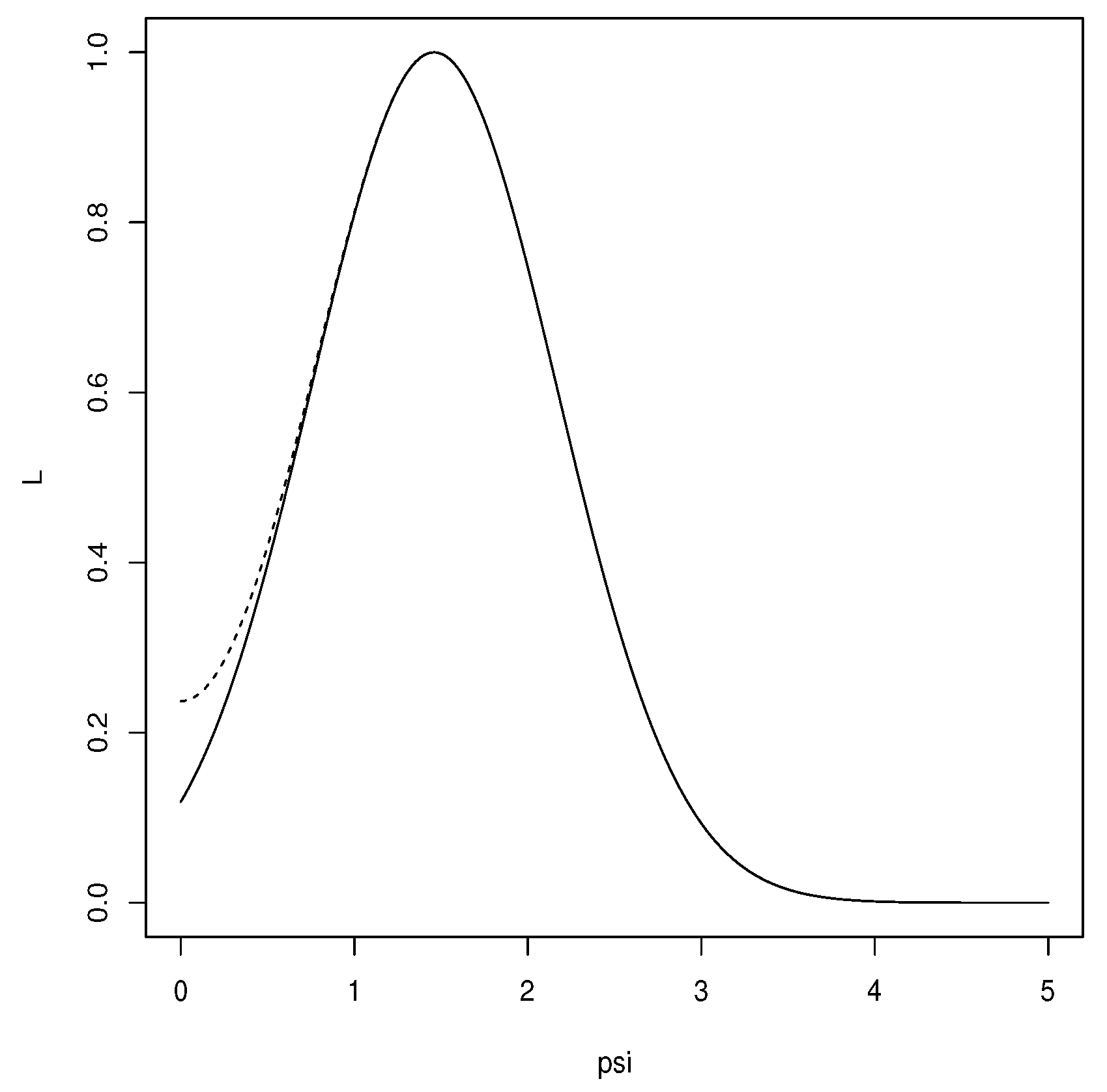
The profile and integrated likelihoods are to be used just as the original likelihood is used for inferences about θ, even though the profile likelihood is not a likelihood. The profile likelihood leads immediately to the estimate $|\overline{x}|$ for ψ, while (2) needs to be maximized numerically. Although the functional forms look quite different, the profile and integrated likelihoods here give almost identical numerical results. Figure 1 is a plot with $n=2,\overline{x}=1.47$ generated from a $N(2,1)$ distribution, and the estimates of ψ are both equal to $1.47.$ There is asome disagreement in the left tail, so some of the reported intervals will differ, but as n increases, such differences disappear. This agreement is also quite robust against the choice of $p.$

Another issue arises with the profile likelihood, namely, the outcome differs in contexts which naturally should lead to equivalent results.

Example 5

(prediction with scale normal). Suppose $x=(x_1,\dots ,x_n)$ is an independent and identically distributed sample from a distribution in the family $\{\varphi (·,0,{\sigma }^2):{\sigma }^2>0\}$. Based on the observed data, the likelihood equals $L\left({\sigma }^2\right|x)={\sigma }^{-n}exp\{-s_x^2/2{\sigma }^2\}$ where $s_x^2={\sum }_{i=1}^n{x_i}^2$ and the MLE of ${\sigma }^2$ is $s_x^2/n.$ Now suppose, however, that the interest is in predicting k future (or occurred but concealed) independent values $y=(y_1,\dots ,y_k)\sim N(0,{\sigma }^2).$ Perhaps the logical predictive likelihood to use is

$$L({\sigma }^2,y|x)={\sigma }^{-(n+k)}exp\{-(s_x^2+s_y^2)/2{\sigma }^2\}$$

where $s_y^2={\sum }_{i=1}^k{y}_i^2.$ Profiling out ${\sigma }^2$ leads to the profile MLE of y equaling 0 for all x as might be expected. Profiling y out of $L({\sigma }^2,y|x),$ however, leads to the profile likelihood

$$L^{prof}\left({\sigma }^2\right|x)={\sigma }^{-(n+k)}exp\{-s_x^2/2{\sigma }^2\}\ne L\left({\sigma }^2\right|x)$$

for ${\sigma }^2$, and so the profile MLE of ${\sigma }_x^2$ equals $s_x^2/(n+k).$

When interest is in ${\sigma }^2,$ the integrated likelihood for ${\sigma }^2$ produces $L\left({\sigma }^2\right|x).$ When interest is in $y,$ then integrating out ${\sigma }^2,$ after placing a probability distribution on ${\sigma }^2$ produces the MLE 0 for y, although the form of the integrated likelihood will depend on the particular distribution chosen.

The profile and integrated likelihoods certainly do not always lead to roughly equivalent results as in Example 4, particularly as the dimension of the nuisance parameters rises. While the profile likelihood has the advantage of not having to specify $\mathsf{\Pi }(·|\psi ),$ it suffers from a lack of a complete justification, at least in terms of the likelihood principle, and, as Example 5 demonstrates, it can produce unnatural results. In Section 3.4, it is shown that the integrated likelihood arises from a very natural principle characterizing evidence.

The discussion here has been mostly about pure likelihood theory, where repeated sampling does not play a role. The likelihood function is also an important aspect of frequentist inference. Such usage, however, does not lead to a resolution of the evidence problem, namely, providing a proper characterization of statistical evidence. In fact, frequentist likelihood methods use the p-value for H. There is no question that the likelihood contains the evidence in the data about $\theta ,$ but questions remain as to how to characterize that evidence, whether in favor of or against a particular value, and also how to express the strength of the evidence. More discussion of the likelihood principle can be found in [25].

3.4. Bayes Factors and Bayesian Measures of Statistical Evidence

Bayesian inference adds another ingredient to the inference base, namely, the prior probability measure $\mathsf{\Pi }$ on $\mathsf{\Theta },$ so now $I=(\mathsf{\Pi },\{f_{\theta }:\theta \in \mathsf{\Theta }\},x).$ The prior represents beliefs about the true value of $\theta .$ Note that $(\mathsf{\Pi },\{f_{\theta }:\theta \in \mathsf{\Theta }\})$ is equivalent to a joint distribution for $(\theta ,x)$ with density $\pi \left(\theta \right)f_{\theta }\left(x\right).$ Once the data x have been observed, a basic principle of inference is then invoked.

Principle of Conditional Probability: for probability model $(\mathsf{\Omega },\mathcal{F},P),$ if $C\in \mathcal{F}$ is observed to be true, where $P\left(C\right)>0,$ then the initial belief that $A\in \mathcal{F}$ is true, as given by $P\left(A\right),$ is replaced by the conditional probability $P\left(A\right|C).$

So, we replace the prior $\pi$ by the posterior $\pi \left(\theta \right|x)=\pi \left(\theta \right)f_{\theta }\left(x\right)/m\left(x\right),$ where $m\left(x\right)={\int }_{\mathsf{\Theta }}\pi \left(\theta \right)f_{\theta }\left(x\right)d\theta$ is the prior predictive density of the data $x,$ to represent beliefs about $\theta .$ While at times the posterior is taken to represent the evidence about $\theta ,$ this confounds two distinct concepts, namely, beliefs and evidence. It is clear, however, that the evidence in the data is what has changed our beliefs, and it is this change that leads to the proper characterization of statistical evidence through the following principle.

Principle of Evidence: for probability model $(\mathsf{\Omega },\mathcal{F},P),$ if $C\in \mathcal{F}$ is observed to be true where $P\left(C\right)>0,$ then there is evidence in favor of $A\in \mathcal{F}$ being true if $P\left(A\right|C)>P(A),$ evidence against $A\in \mathcal{F}$ being true if $P\left(A\right|C)<P(A)$ and no evidence either way if $P\left(A\right|C)=P(A).$

Therefore, in the Bayesian context, we compare $\pi \left(\theta \right|x)$ with $\pi \left(\theta \right)$ to determine whether or not there is evidence one way or the other concerning $\theta$ being the true value. This seems immediate in the context where $\mathsf{\Pi }$ is a discrete probability measure. It is also relevant in the continuous case, where densities are defined via limits, as in $\pi \left(\theta \right)={lim}_{ϵ\to 0}\mathsf{\Pi }\left(N_{ϵ}\left(\theta \right)\right)/\nu \left(N_{ϵ}\left(\theta \right)\right)$, where $N_{ϵ}\left(\theta \right)$ is a sequence of neighborhoods of $\theta$ converging nicely to $\theta$ as $ϵ\to 0$, and $\mathsf{\Pi }$ is absolutely continuous with respect to support measure $\nu .$ This leads to the usual expressions for densities; see [26] (Appendix A) for details.

The Bayesian formulation has a very satisfying consistency property. If interest is in the parameter $\psi =\mathsf{\Psi }\left(\theta \right),$ then the nuisance parameters can be integrated out using the conditional prior $\mathsf{\Pi }(·|\psi )$ and the inference base $I=(\mathsf{\Pi },\{f_{\theta }:\theta \in \mathsf{\Theta }\},x)$ is replaced by $I_{\mathsf{\Psi }}=({\mathsf{\Pi }}_{\mathsf{\Psi }},\{m(·|\psi ):\psi \in \mathsf{\Psi }\left(\mathsf{\Theta }\right)\},x)$ where ${\mathsf{\Pi }}_{\mathsf{\Psi }}$ is the marginal prior on $\psi$, with density ${\pi }_{\mathsf{\Psi }}.$ Applying the principal of evidence here means to compare the posterior

$${\pi }_{\mathsf{\Psi }}\left(\psi \right|x)={\pi }_{\mathsf{\Psi }}\left(\psi \right){\displaystyle \frac{m\left(x\right|\psi )}{m\left(x\right)}}={\int }_{{\mathsf{\Psi }}^{-1}\left\{\psi \right\}}\mathsf{\Pi }\left(d\theta \right|x)$$

(3)

to the prior density ${\pi }_{\mathsf{\Psi }}\left(\psi \right)={\int }_{{\mathsf{\Psi }}^{-1}\left\{\psi \right\}}\mathsf{\Pi }\left(d\theta \right).$ So, there is evidence in favor of $\psi$ being the true value whenever ${\pi }_{\mathsf{\Psi }}\left(\psi \right|x)>{\pi }_{\mathsf{\Psi }}\left(\psi \right),$ etc.

In many applications, we need more than the simple characterization of evidence that the principle of evidence gives us. A valid measure of evidence is then any real-valued function of $I_{\mathsf{\Psi }}$ that satisfies the existence of a cut-off c such that the function taking a value greater than c corresponds to evidence in favor, etc. One very simple function satisfying this is the relative belief ratio

$$R{B}_{\mathsf{\Psi }}\left(\psi \right|x)={\displaystyle \frac{{\pi }_{\mathsf{\Psi }}\left(\psi \right|x)}{{\pi }_{\mathsf{\Psi }}\left(\psi \right)}}={\displaystyle \frac{m\left(x\right|\psi )}{m\left(x\right)}}$$

(4)

where the second equality follows from (3) and is sometimes referred to as the Savage–Dickey ratio; see [27]. Using $R{B}_{\mathsf{\Psi }}\left(\psi \right|x)$, the values of $\psi$ are now totally ordered with respect to evidence, as when $1<R{B}_{\mathsf{\Psi }}\left({\psi }_1\right|x)<R{B}_{\mathsf{\Psi }}\left({\psi }_2\right|x)$, there is more evidence in favor of ${\psi }_2$ than for ${\psi }_1,$ etc.

This suggests an immediate answer to E, namely, record the relative belief estimate $\psi \left(x\right)=arg{sup}_{\psi }R{B}_{\mathsf{\Psi }}\left(\psi \right|x)$, as this value has the maximum evidence in its favor. Also, to assess the accuracy of $\psi \left(x\right)$, record the plausible region $P{l}_{\mathsf{\Psi }}\left(x\right)=\{\psi :R{B}_{\mathsf{\Psi }}\left(\psi \right|x)>1\}$, the set of $\psi$ values with evidence in their favor, together with its posterior content ${\mathsf{\Pi }}_{\mathsf{\Psi }}\left(P{l}_{\mathsf{\Psi }}\left(x\right)\right|x)$, as this measures the belief that the true value is in $P{l}_{\mathsf{\Psi }}\left(x\right).$ Note that while $\psi \left(x\right)$ depends on the choice of the relative belief ratio to measure evidence, the plausible region $P{l}_{\mathsf{\Psi }}\left(x\right)$ only depends on the principle of evidence. This suggests that any other valid measure of evidence can be used instead to determine an estimate, as it will lie in $P{l}_{\mathsf{\Psi }}\left(x\right)$. A $\gamma$-credible region $C_{\mathsf{\Psi },\gamma }\left(x\right)$ for $\psi$ can also be quoted based on any valid measure of evidence provided $C_{\mathsf{\Psi },\gamma }\left(x\right)\subset P{l}_{\mathsf{\Psi }}\left(x\right)$, as, otherwise, $C_{\mathsf{\Psi },\gamma }\left(x\right)$ would contain a value of $\psi$ for which there is evidence against $\psi$ being the true value. For example, a relative belief $\gamma$-credible region takes the form $C_{\mathsf{\Psi },\gamma }\left(x\right)=\{\psi :R{B}_{\mathsf{\Psi }}\left(\psi \right|x)\ge c_{\gamma }\left(x\right)\}$ where $c_{\gamma }\left(x\right)=inf\{c:$${\mathsf{\Pi }}_{\mathsf{\Psi }}(R{B}_{\mathsf{\Psi }}\left(\psi \right|x)\le c|x)\ge 1-\gamma \}.$

For H, the value $R{B}_{\mathsf{\Psi }}\left({\psi }_0\right|x)$ tells us immediately whether there is evidence in favor of or against $H_0:\mathsf{\Psi }\left(\theta \right)={\psi }_0.$ To measure the strength of the evidence concerning $H_0$, there is the posterior probability ${\mathsf{\Pi }}_{\mathsf{\Psi }}\left(\left\{{\psi }_0\right\}\right|x),$ as this measures our belief in what the evidence says. If $R{B}_{\mathsf{\Psi }}\left({\psi }_0\right|x)>1$ and ${\mathsf{\Pi }}_{\mathsf{\Psi }}\left(\left\{{\psi }_0\right\}\right|x)\approx 1,$ then there is strong evidence that $H_0$ is true, while when $R{B}_{\mathsf{\Psi }}\left({\psi }_0\right|x)<1$ and ${\mathsf{\Pi }}_{\mathsf{\Psi }}\left(\left\{{\psi }_0\right\}\right|x)\approx 0,$ then there is strong evidence that $H_0$ is false. Often, however, ${\mathsf{\Pi }}_{\mathsf{\Psi }}\left(\left\{{\psi }_0\right\}\right|x)$ will be small, even 0 in the continuous case, so it makes more sense to measure the strength of the evidence in such a case by $St{r}_{\mathsf{\Psi }}\left({\psi }_0\right)={\mathsf{\Pi }}_{\mathsf{\Psi }}(R{B}_{\mathsf{\Psi }}\left(\psi \right|x)\le R{B}_{\mathsf{\Psi }}\left({\psi }_0\right|x)|x)$, as when $R{B}_{\mathsf{\Psi }}\left({\psi }_0\right|x)>1$ and $St{r}_{\mathsf{\Psi }}\left({\psi }_0\right)\approx 1,$ then there is small belief that the true value of $\psi$ has more evidence in its favor than ${\psi }_0,$ etc.

Recalling the discussion in Section 3.1 about the difference that matters $\delta ,$ it is relatively easy to take this into account in this context, at least when $\psi$ is real valued. For this, we consider a grid of values $\dots {\psi }_{-2},{\psi }_{-1},{\psi }_0,{\psi }_1,{\psi }_2,\dots$ separated by $\delta$ and then conduct the inferences using the relative belief ratios of the intervals $[{\psi }_i-\delta /2,{\psi }_i+\delta /2).$ In effect, $H_0$ is now $H_0:\mathsf{\Psi }\left(\theta \right)\in [{\psi }_0-\delta /2,{\psi }_0+\delta /2).$

Example 6

(location normal). Suppose that we add the prior $\mu \sim N({\mu }_0,{\tau }_0^2)$ to form a Bayesian inference base. The posterior distribution is then

$$\mu |x\sim N\left({\left(n/{\sigma }_0^2+1/{\tau }_0^2\right)}^{-1}(n\overline{x}/{\sigma }_0^2+{\mu }_0/{\tau }_0^2),{\left(n/{\sigma }_0^2+1/{\tau }_0^2\right)}^{-1}\right).$$

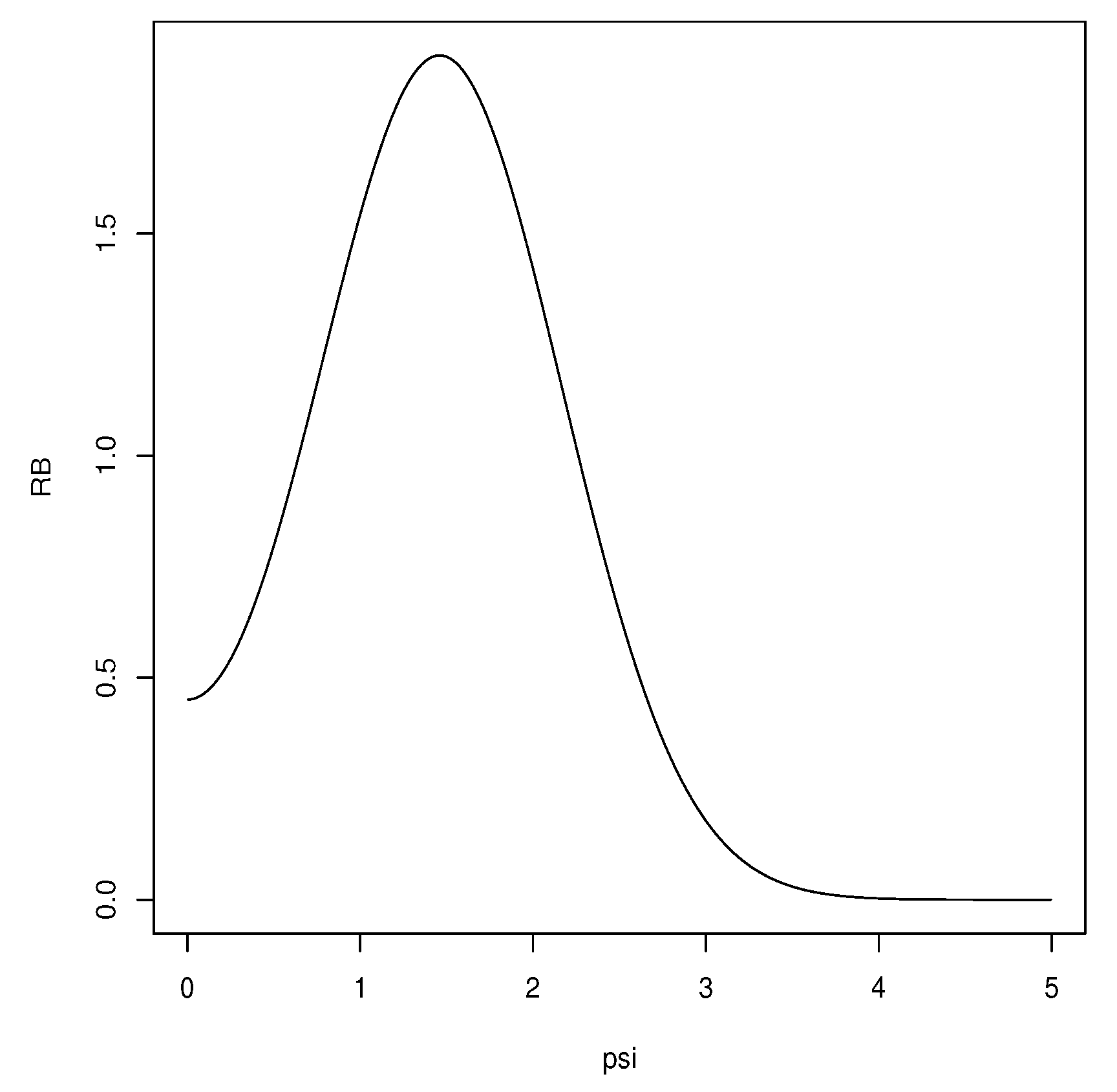
Suppose our interest is inference about $\psi =\mathsf{\Psi }\left(\mu \right)=\left|\mu \right|.$ Figure 2 is a plot of the relative belief ratio based on the data in Example 4 $(n=2,\overline{x}=1.47$ generated from a $N(2,1)$ distribution) and using the prior with ${\mu }_0=0,{\tau }_0=2.$ From (4), it is seen that maximizing $R{B}_{\mathsf{\Psi }}\left(\psi \right|x)$ is equivalent to maximizing the integrated likelihood, and in this case, the prior is such that $sgn\left(\mu \right)=1$ with prior probability 0.5, so indeed the relative belief estimate is $\psi \left(x\right)=1.47.$ To assess the accuracy of the estimate, we record the plausible interval $P{l}_{\mathsf{\Psi }}\left(x\right)=(0.65,2.26)$ which has posterior content $0.76.$ There is evidence in favor of $H_0:\psi =2$ since $2\in P{l}_{\mathsf{\Psi }}\left(x\right),$ and $R{B}_{\mathsf{\Psi }}\left(2\right|x)=1.41$ with $St{r}_{\mathsf{\Psi }}\left({\psi }_0\right)=0.42,$ so there is only moderate evidence in favor of 2 being the true value of ψ. Of course, these results improve with sample size $n.$ For example, for $n=10,\psi \left(x\right)=1.83$ with $P{l}_{\mathsf{\Psi }}\left(x\right)=(1.40,2.27)$ with posterior content $0.95$ and $R{B}_{\mathsf{\Psi }}\left(2\right|x)=5.00$ with strength $0.44.$ So, the plausible interval has shortened considerably, and its posterior content has substantially increased, but the strength of the evidence in favor of $H_0:\psi =2$ has not increased by much. It is important to note that, because we are employing a discretization (with $\delta =0.01$ here), and since the posterior is inevitably virtually completely concentrated in $[{\psi }_0-\delta /2,{\psi }_0+\delta /2)$ as $n\to \infty ,$ the strength $St{r}_{\mathsf{\Psi }}\left(2\right)$ converges to 1 at any of the values in this interval and to 0 at values outside of it.

There are a number of optimal properties for the relative belief inferences as discussed in [26]. While this is perhaps the first attempt to build a theory of inference based on the principle of evidence, there is considerable literature on this idea in the philosophy of science where it underlies what is known as confirmation theory; see [28]. For example, the philosopher Popper in [29] (Appendix ix) writes

If we are asked to give a criterion of the fact that the evidence y supports or corroborates a statement x, the most obvious reply is: that y increases the probability of $x.$

One issue with philosophers’ discussions is that these are never cast in a statistical context. Many of the anomalies raised in those discussions, such as Hempel’s Raven Paradox, can be resolved when formulated as statistical problems. Also, the relative belief ratio itself has appeared elsewhere, although under different names, as a natural measure of evidence.

There are indeed other valid measures of evidence besides the relative belief ratio, for example, the Bayes factor originated with Jeffreys as in [30]; see [6,31] for discussion. For probability model $(\mathsf{\Omega },\mathcal{F},P),A,C\in \mathcal{F}$ with $P\left(A\right)>0,P\left(C\right)>0,$ the Bayes factor in favor of A being true, after observing that C is true, is given by

$$BF\left(A\right|C)={\displaystyle \frac{P\left(A\right|C)/P\left(A^c\right|C)}{P\left(A\right)/P\left(A^c\right)}},$$

the ratio of the posterior odds in favor of $A$ to the prior odds in favor of $A.$ It is immediate that $BF\left(A\right|C)$ is a valid measure of evidence because $BF\left(A\right|C)>1$ if and only if $P\left(A\right|C)>P(A).$ Also, $BF\left(A\right|C)=RB\left(A\right|C)/RB\left(A^c\right|C)$ and so, because $RB\left(A\right|C)>1$ if and only if $RB\left(A^c\right|C)<1,$ this implies $BF\left(A\right|C)>RB(A\left|C\right)$ when there is evidence in favor and $BF\left(A\right|C)<RB(A\left|C\right)$ when there is evidence against. These inequalities are important because it is sometimes asserted that the Bayes factor is not only a measure of evidence but also that its value is a measure of the strength of that evidence.

Table 1. Jeffreys’ Bayes factor scale for measuring strength of the evidence in favor (the strength of evidence against is measured by the reciprocals).

Bayes Factor	Strength
1 to ${10}^{1/2}$	Barely worth mentioning
${10}^{1/2}$ to 10	Substantial
10 to ${10}^{3/2}$	Strong
${10}^{3/2}$ to ${10}^2$	Very Strong
>${10}^2$	Decisive

gives a scale, due to Jeffreys (see [32] (Appendix B), which supposedly can be used to assess the strength of evidence as given by the Bayes factor. Again, this is an attempt to establish a universal scale on which evidence can be measured and currently no grounds exist for claiming that such a scale exists. If we consider that the strength of the evidence is to be measured by how strongly we believe what the evidence says, then simple examples can be constructed to show that such a scale is inappropriate. Effectively, the strength of the evidence is context dependent and needs to be calibrated.

Example 7.

Suppose Ω is a set with $\#\left(\mathsf{\Omega }\right)=N.$ A value ω is generated uniformly from Ω and partially concealed but it is noted that $\omega \in C$ where $\#\left(C\right)=n.$ It is desired to know if $\omega \in A$ where $\#\left(A\right)=1$ and $A\subset C.$ Then, we have that $P\left(A\right)=1/N$ and $P\left(A\right|C)=1/n$ so $RB\left(A\right|C)=N/n>1$ since $n<N.$ The posterior belief in what the evidence is saying is, however, $P\left(A\right|C)=1/n$ which can be very small, say when $n={10}^3.$ But, if $N={10}^6,$ then $BF\left(A\right|C)>RB\left(A\right|C)={10}^3$ which is well into the range where Jeffreys scale says it is decisive evidence in favor of $A.$ Clearly there is only very weak evidence in favor of A being true here. Also, note that the posterior probability by itself does not indicate evidence in favor although the observation that C is true must be evidence in favor of A because $A\subset C.$ The example can obviously be modified to show that any such scale is not appropriate.

There is another issue with current usage of the Bayes factor that needs to be addressed. This arises when interest is in assessing the evidence for or against $H_0:\mathsf{\Psi }\left(\theta \right)={\psi }_0$ when ${\mathsf{\Pi }}_{\mathsf{\Psi }}\left(\left\{{\psi }_0\right\}\right)=0.$ Clearly, the Bayes factor is not defined in such a context. An apparent solution is provided by choosing a prior of the form ${\mathsf{\Pi }}_{H_0,p}=p{\mathsf{\Pi }}_{H_0}+(1-p)\mathsf{\Pi }$, where $p>0$ is a prior probability assigned to $H_0$, and ${\mathsf{\Pi }}_{H_0}$ is a prior probability measure on the set ${\mathsf{\Psi }}^{-1}\left\{{\psi }_0\right\}.$ Since ${\mathsf{\Pi }}_p\left({\mathsf{\Psi }}^{-1}\left\{{\psi }_0\right\}\right)=p$ the Bayes factor is now defined. Of some concern now is how ${\mathsf{\Pi }}_{H_0}$ should be chosen. A natural choice is to take ${\mathsf{\Pi }}_{H_0}=\mathsf{\Pi }(·|{\psi }_0)$ otherwise there is a contradiction between beliefs as expressed by $\mathsf{\Pi }$ and ${\mathsf{\Pi }}_{H_0}.$ It follows very simply, however, that in the continuous case, when ${\mathsf{\Pi }}_{H_0}=\mathsf{\Pi }(·|{\psi }_0),$ then $BF\left({\psi }_0\right|x)=R{B}_{\mathsf{\Psi }}\left({\psi }_0\right|x).$ Moreover, if instead of using such a mixture prior, we define the Bayes factor via

$$B{F}_{\mathsf{\Psi }}\left({\psi }_0\right|x)=\underset{ϵ\to 0}{lim}BF\left(N_{ϵ}\left({\psi }_0\right)\right|x)=\underset{ϵ\to 0}{lim}{\displaystyle \frac{{\mathsf{\Pi }}_{\mathsf{\Psi }}\left(N_{ϵ}\left({\psi }_0\right)\right|x)/{\mathsf{\Pi }}_{\mathsf{\Psi }}\left(N_{ϵ}^c\left({\psi }_0\right)\right|x)}{{\mathsf{\Pi }}_{\mathsf{\Psi }}\left(N_{ϵ}\left({\psi }_0\right)\right)/{\mathsf{\Pi }}_{\mathsf{\Psi }}\left(N_{ϵ}^c\left({\psi }_0\right)\right)}},$$

where $N_{ϵ}\left({\psi }_0\right)$ is a sequence of neighborhoods of ${\psi }_0$ converging nicely to ${\psi }_0,$ then, under weak conditions (${\pi }_{\mathsf{\Psi }}$ is positive and continuous at ${\psi }_0)$, $B{F}_{\mathsf{\Psi }}\left({\psi }_0\right|x)=R{B}_{\mathsf{\Psi }}\left({\psi }_0\right|x).$ So, there is no need to introduce the mixture prior to get a valid measure of evidence. Furthermore, now the Bayes factor is available for E as well as H as surely any proper characterization of statistical evidence must be, and the relevant posterior for $\psi$ is ${\mathsf{\Pi }}_{\mathsf{\Psi }}(·|x)$ as obtained from $\mathsf{\Pi }$ rather than from ${\mathsf{\Pi }}_{H_0,p}.$

Other Bayesian measures of evidence have been proposed. For example, it is proposed in [33] to measure the evidence for $H_0:\mathsf{\Psi }\left(\theta \right)={\psi }_0$ by computing ${\theta }_{*}=arg{sup}_{\mathsf{\Psi }\left(\theta \right)={\psi }_0}\pi \left(\theta \right|x)$ and then use the posterior tail probability $ev\left(H_0\right|x)=\mathsf{\Pi }(\pi \left(\theta \right|x)\le \pi \left({\theta }_{*}\right|x)|x).$ If $ev\left(H_0\right|x)$ is large, this is evidence against $H_0$, while, if it is small, it is evidence in favor of $H_0$. Note that $ev\left(H_0\right|x)$ is sometimes referred to as an e-value, but this is different from the e-values discussed in Section 3.1. Further discussion and development of this concept can be found in [34]. Clearly, this is building on the idea that underlies the p-value, namely, providing a measure that locates a point in a distribution and using this to assess evidence. It does not, however, conform to the principle of evidence.

Bias and Error Probabilities

One criticism that is made of Bayesian inference is that there are no measures of reliability of the inferences, which is an inherent part of frequentism. It is natural to add such measures, however, to assess whether or not the specified model and prior could potentially lead to misleading inferences. For example, suppose it could be shown that evidence in favor of $H_0:\mathsf{\Psi }\left(\theta \right)={\psi }_0$ would be obtained with prior probability near 1, for a data set of given size. It seems obvious that, if we did collect this amount of data and obtained evidence in favor of $H_0,$ then this fact would undermine our confidence in the reliability of the reported inference.

Example 8

(Jeffreys–Lindley paradox). Suppose we have the location normal model $\overline{x}\sim N(\mu ,{\sigma }_0^2/n)$ and $T_{{\mu }_0}\left(x\right)=\sqrt{n}|\overline{x}-{\mu }_0|/{\sigma }_0=5$ is obtained which leads to the p-value $2(1-\mathsf{\Phi }(\sqrt{n}|\overline{x}-{\mu }_0|/{\sigma }_0\left)\right)=5.733031\times {10}^{-7}$, so there would appear to be definitive evidence that $H_0:\mu ={\mu }_0$ is false. Suppose the prior $\mu \sim N({\mu }_0,{\tau }_0^2)$ is used, and the analyst chooses ${\tau }_0^2$ to be very large to reflect the fact that little is known about the true value of $\mu .$ It can be shown (see [26]), however, that $R{B}_{\mathsf{\Psi }}\left({\mu }_0\right|x)\to \infty$ as ${\tau }_0^2\to \infty .$ Therefore, for a very diffuse prior, evidence in favor of $H_0$ will be obtained, and so the frequentist and Bayesian will disagree. Note that the Bayes factor equals the relative belief ratio in this context. A partial resolution of this contradiction is obtained by noting that $St{r}_{\mathsf{\Psi }}\left({\mu }_0\right)\to 2(1-\mathsf{\Phi }(\sqrt{n}|\overline{x}-{\mu }_0|/{\sigma }_0\left)\right)$ as ${\tau }_0^2\to \infty$ and so the Bayesian measure of evidence is only providing very weak evidence when the p-value is small. This anomaly occurs even when the true value of μ is indeed far away from ${\mu }_0$, and so the fault here does not lie with the p-value.

Prior error probabilities associated with Bayesian measures of evidence can, however, be computed and these lead to a general resolution of the apparent paradox. There are two error probabilities for H that we refer to as bias against $H_0$ and bias in favor of $H_0$ as given by the following two prior probabilities

$$\begin{array}{cc}\hfill & \mathit{bias}{\mathit{against}}_{\mathsf{\Psi }}\left({\psi }_0\right)=M(R{B}_{\mathsf{\Psi }}\left({\psi }_0\right|X)\le 1|{\psi }_0),\hfill \\ \hfill & \mathit{bias}\mathit{in}{\mathit{favor}}_{\mathsf{\Psi }}\left({\psi }_0\right)=\underset{\psi :d_{\mathsf{\Psi }}(\psi ,{\psi }_0)\ge \delta }{sup}M(R{B}_{\mathsf{\Psi }}\left({\psi }_0\right|X)\ge 1|\psi ).\hfill \end{array}$$

Both of these biases are independent of the valid measure of evidence used, as they only depend on the principle of evidence as applied to the model and prior chosen. The $\mathit{bias}{\mathit{against}}_{\mathsf{\Psi }}\left({\psi }_0\right)$ is the prior probability of not getting evidence in favor of ${\psi }_0$ when it is true and plays a role similar to type I error. The $\mathit{bias}\mathit{in}{\mathit{favor}}_{\mathsf{\Psi }}\left({\psi }_0\right)$ is the prior probability of not obtaining evidence against ${\psi }_0$ when it is meaningfully false and plays a role similar to that of the type II error. Here, $\delta$ is the deviation from ${\psi }_0$ which is of scientific interest as determined by some measure of distance $d_{\mathsf{\Psi }}$ on $\mathsf{\Psi }\left(\mathsf{\Theta }\right).$ As discussed in [26], these biases cannot be controlled by, for example, the choice of prior, as a prior that reduces $\mathit{bias}{\mathit{against}}_{\mathsf{\Psi }}\left({\psi }_0\right)$ causes $\mathit{bias}\mathit{in}{\mathit{favor}}_{\mathsf{\Psi }}\left({\psi }_0\right)$ to increase and vice versa. The proper control of these quantities is through sample size as both converge to 0 as $n\to \infty .$

Example 9

(Jeffreys–Lindley paradox). In this case, bias against $\left({\psi }_0\right)\to 0$ and the bias in favor of $\left({\psi }_0\right)\to 1$ as ${\tau }_0^2\to \infty .$ This leads to an apparent resolution of the issue: do not choose the prior to be arbitrarily diffuse to reflect noninformativeness; rather, choose a prior that is sufficiently diffuse to cover the interval where it is known μ must lie, e.g., the interval where the measurements lie, and then choose n so that both biases are suitably small. While the Jeffreys–Lindley paradox arises due to diffuse priors inducing bias in favor, an overly concentrated prior induces bias against, but again this bias can be controlled via the amount of data collected.

There are also two biases associated with E obtained by averaging, using the prior ${\mathsf{\Pi }}_{\mathsf{\Psi }},$ the biases for H. These can also be expressed in terms of coverage probabilities of the plausible region $P{l}_{\mathsf{\Psi }}\left(x\right).$ The biases for E are given by

$$\begin{array}{cc}\hfill & E_{{\mathsf{\Pi }}_{\mathsf{\Psi }}}\left(\mathit{bias}{\mathit{against}}_{\mathsf{\Psi }}\right)=E_{{\mathsf{\Pi }}_{\mathsf{\Psi }}}\left(M(R{B}_{\mathsf{\Psi }}\left(\psi \right|X)\le 1|\psi )\right)=E_{{\mathsf{\Pi }}_{\mathsf{\Psi }}}\left(M(\psi \notin P{l}_{\mathsf{\Psi }}\left(X\right)|\psi )\right),\hfill \\ \hfill & E_{{\mathsf{\Pi }}_{\mathsf{\Psi }}}\left(\mathit{bias}\mathit{in}{\mathit{favor}}_{\mathsf{\Psi }}\right)=E_{{\mathsf{\Pi }}_{\mathsf{\Psi }}}\left(\underset{{\psi }^{\prime }:d_{\mathsf{\Psi }}({\psi }^{\prime },\psi )\ge \delta }{sup}M(R{B}_{\mathsf{\Psi }}\left(\psi \right|X)\ge 1|{\psi }^{\prime })\right)\hfill \\ \hfill & =E_{{\mathsf{\Pi }}_{\mathsf{\Psi }}}\left(\underset{{\psi }^{\prime }:d_{\mathsf{\Psi }}({\psi }^{\prime },\psi )\ge \delta }{sup}M(\psi \notin I{m}_{\mathsf{\Psi }}\left(X\right)|{\psi }^{\prime })\right)\hfill \end{array}$$

where $I{m}_{\mathsf{\Psi }}\left(x\right)=\{\psi :R{B}_{\mathsf{\Psi }}\left(\psi \right|x)<1\}$ is the implausible region, namely, the set of values for which evidence against has been obtained. So, $E_{{\mathsf{\Pi }}_{\mathsf{\Psi }}}\left(\mathit{bias}{\mathit{against}}_{\mathsf{\Psi }}\right)$ is the prior probability that the true value is not in the plausible region $P{l}_{\mathsf{\Psi }}\left(x\right)$ and so $1-E_{{\mathsf{\Pi }}_{\mathsf{\Psi }}}\left(M(\psi \notin P{l}_{\mathsf{\Psi }}\left(X\right)|\psi )\right)$ is the prior coverage probability (Bayesian confidence) of $P{l}_{\mathsf{\Psi }}\left(x\right).$ It is of interest that there is typically a value ${\psi }_{*}=arg{sup}_{\psi }\mathit{bias}{\mathit{against}}_{\mathsf{\Psi }}\left(\psi \right)$ and so

$$M(\psi \in P{l}_{\mathsf{\Psi }}\left(X\right)|\psi )\ge 1-M(R{B}_{\mathsf{\Psi }}\left({\psi }_{*}\right|X)\le 1|{\psi }_{*})$$

gives a lower bound on the frequentist confidence of $P{l}_{\mathsf{\Psi }}\left(x\right)$ with respect to the model $\left\{m\right(·\left|\psi \right):\psi \in \mathsf{\Psi }\}$ obtained from the original model by integrating out the nuisance parameters. In both cases, the Bayesian confidences are average frequentist confidences with respect to the original model. $E_{{\mathsf{\Pi }}_{\mathsf{\Psi }}}\left(\mathit{bias}\mathit{in}{\mathit{favor}}_{\mathsf{\Psi }}\right)$ is the prior probability that a meaningfully false value is not in the implausible region. Again, both of these biases do not depend on the valid measure of statistical evidence used and converge to 0 with increasing sample size.

With the addition of the biases, a link is established between Bayesianism and frequentism: inferences are Bayesian, but the reliability of the inferences is assessed via frequentist criteria. More discussion on bias in this context can be found in [35].

4. Conclusions

This paper is a review of various conceptions of statistical evidence, as this has been discussed in the literature. It is seen that precisely characterizing evidence is still an unsolved problem in purely frequentist inference and in pure likelihood theory, but the Bayesian framework provides a natural way to perform this through the principle of evidence. One often hears complaints about the need to choose a prior which can be performed properly through elicitation; see [36]. Furthermore, priors are falsifiable via checking for prior-data conflict; see [26]. Finally, the effects of priors can be mitigated by the control of the biases, which are directly related to the principle of evidence.

References

- Ionides, E.L.; Giessing, A.; Ritov, Y.; Page, S.E. Response to the ASA’s Statement on p-Values: Context, Process, and Purpose. Am. Stat. 2017, 71, 88–89. [Google Scholar] [CrossRef]
- Wasserstein, R.L.; Lazar, N.A. The ASA Statement on p-Values: Context, process, and purpose. Am. Stat. 2016, 70, 129–133. [Google Scholar] [CrossRef]
- Lehmann, E.L. Neyman’s statistical philosophy. In Selected Works of E. L. Lehmann; Springer: Boston, MA, USA, 1995; pp. 1067–1073. [Google Scholar]
- Neyman, J. “Inductive Behavior” as a basic concept of philosophy of science. Rev. Int. Stat. Inst. 1957, 25, 7–22. [Google Scholar] [CrossRef]
- Neyman, J. Foundations of behavioristic statistics. In Foundations of Statistical Inference, a Symposium; Godambe, V.P., Sprott, D.A., Eds.; Holt, Rinehart and Winston of Canada: Toronto, ON, Canada, 1971; pp. 1–13. [Google Scholar]
- Berger, J.O. Statistical Decision Theory and Bayesian Analysis, 2nd ed.; Springer: Berlin/Heidelberg, Germany, 2006. [Google Scholar]
- Fisher, R.A. Statistical Methods for Research Workers, 14th ed.; Hafner Press: Royal Oak, MI, USA, 1925. [Google Scholar]
- Stigler, S.M. The History of Statistics; Belknap Press: Cambridge, MA, USA, 1986. [Google Scholar]
- Stigler, S.M. The Seven Pillars of Statistical Wisdom; Harvard University Press: Cambridge, MA, USA, 2016. [Google Scholar]
- Royall, R. Statistical Evidence: A likelihood paradigm; Chapman & Hall: London, UK, 1997. [Google Scholar]
- Ioannidis, J.P.A. The proposal to lower p-value thresholds to .005. J. Am. Med. Assoc. 2018, 319, 1429–1430. [Google Scholar] [CrossRef] [PubMed]
- Boring, E.G. Mathematical vs. scientific significance. Psychol. Bull. 1919, 16, 335–338. [Google Scholar] [CrossRef]
- Cornfield, J. Sequential trials, sequential analysis and the likelihood principle. Am. Stat. 1966, 20, 18–23. [Google Scholar] [CrossRef]
- Grunwald, P.; de Heide, R.; Koolen, W.M. Safe testing. J. R. Stat. Soc. Ser. B 2024, in press. [Google Scholar] [CrossRef]
- Shafer, G.; Shafer, A.; Vereshchagin, N.; Vovk, V. Test martingales, Bayes factors and p-values. Stat. Sci. 2011, 26, 84–101. [Google Scholar]
- Vovk, V.; Wang, R. Confidence and discoveries with e-values. Stat. Sci. 2023, 38, 329–354. [Google Scholar] [CrossRef]
- Birnbaum, A. On the foundations of statistical inference (with discussion). J. Am. Stat. Assoc. 1962, 57, 269–326. [Google Scholar] [CrossRef]
- Birnbaum, A. The Neyman-Pearson theory as decision theory, and as inference theory; with criticism of the Lindley-Savage argument for Bayesian theory. Synthese 1977, 36, 19–49. [Google Scholar] [CrossRef]
- Giere, R.N. Publications by Allan Birnbaum. Synthese 1977, 36, 15–17. [Google Scholar] [CrossRef]
- Evans, M. What does the proof of Birnbaum’s theorem prove? Electron. J. Stat. 2013, 7, 2645–2655. [Google Scholar] [CrossRef]
- Evans, M.; Frangakis, C. On resolving problems with conditionality and its implications for characterizing statistical evidence. Sankhya A 2023, 85, 1103–1126. [Google Scholar] [CrossRef]
- Fisher, R.A. On the mathematical foundations of theoretical statistics. Philos. Trans. R. Soc. London. Ser. A 1922, 222, 309–368. [Google Scholar]
- Edwards, A.W.F. Likelihood, 2nd ed.; Johns Hopkins University Press: Baltimore, MD, USA, 1992. [Google Scholar]
- Berger, J.O.; Liseo, B.; Wolpert, R.L. Integrated likelihood methods for eliminating nuisance parameters. Stat. Sci. 1999, 14, 1–22. [Google Scholar] [CrossRef]
- Berger, J.O.; Wolpert, R.L. The Likelihood Principle: A Review, Generalizations, and Statistical Implications. IMS Lecture Notes Monogr. Ser. 1988, 6, 208. [Google Scholar] [CrossRef]
- Evans, M. Measuring Statistical Evidence Using Relative Belief. CRC Press: Boca Raton, FL, USA, 2015. [Google Scholar]
- Dickey, J. The weighted likelihood ratio, linear hypotheses on normal location parameters. Ann. Stat. 1971, 42, 204–223. [Google Scholar] [CrossRef]
- Salmon, W. Confirmation. Sci. Am. 1973, 228, 75–81. [Google Scholar] [CrossRef]
- Popper, K. The Logic of Scientific Discovery. Harper Torchbooks; Routledge: New York, NY, USA, 1968. [Google Scholar]
- Jeffreys, H. Some tests of significance, treated by the theory of probability. Math. Proc. Camb. Philos. 1935, 31, 203–222. [Google Scholar] [CrossRef]
- Kass, R.E.; Raftery, A.E. Bayes factors. J. The American Stat. Assoc. 1995, 90, 773–795. [Google Scholar] [CrossRef]
- Jeffreys, H. Theory of Probability, 3rd ed.; Oxford University Press BPS: Oxford, UK, 1961. [Google Scholar]
- De Bragança Pereira, C.A.; Stern, J.M. Evidence and credibility: Full Bayesian significance test for precise hypotheses. Entropy 1999, 1, 99–110. [Google Scholar] [CrossRef]
- Stern, J.M.; Pereira, C.A.D.B.; Lauretto, M.D.S.; Esteves, L.G.; Izbicki, R.; Stern, R.B.; Diniz, M. The e-value and the full Bayesian significance test: Logical properties and philosophical consequences. São Paulo J. Math. Sci. 2022, 16, 566–584. [Google Scholar]
- Evans, M.; Guo, Y. Measuring and controlling bias for some Bayesian inferences and the relation to frequentist criteria. Entropy 2021, 23, 190. [Google Scholar] [CrossRef] [PubMed]
- O’Hagan, A.; Buck, C.E.; Daneshkhah, A.; Eiser, J.R.; Garthwaite, P.H.; Jenkinson, D.J.; Oakley, J.E.; Rakow, T. Uncertain Judgements: Eliciting Expert Probabilities; Wiley: Hoboken, NJ, USA, 2006. [Google Scholar]
Disclaimer/Publisher’s Note: The statements, opinions and data contained in all publications are solely those of the individual author(s) and contributor(s) and not of MDPI and/or the editor(s). MDPI and/or the editor(s) disclaim responsibility for any injury to people or property resulting from any ideas, methods, instructions or products referred to in the content. |
© 2024 by the author. Licensee MDPI, Basel, Switzerland. This article is an open access article distributed under the terms and conditions of the Creative Commons Attribution (CC BY) license (https://creativecommons.org/licenses/by/4.0/).