1. Introduction
Spin Hamiltonians are used to model the properties of exchange-coupled magnetic solids and molecules, particularly those of the first transition-metal series [
1], such as magnetic susceptibilities and heat capacities or magnetic-resonance and neutron-scattering spectra. Based on matrix diagonalization, all physical quantities within the framework of the model can be calculated exactly. While the Hilbert space grows exponentially with the number of centers, the system size limit for numerically exact or quasi-exact calculations [
2] can be increased by taking advantage of symmetries [
3,
4,
5,
6,
7,
8,
9,
10,
11]. However, for simulating large systems, various approximations are essential [
12].
On the opposite side of the range, small clusters allow closed-form solutions, especially if the Hamiltonian is isotropic and invariant with respect to spin permutations [
8] corresponding to spatial symmetries of the molecule or cluster. In addition to their pedagogical value, analytical solutions yield insights that might be obscured or unavailable in numerical data. For example, they can facilitate parametric plots of spectra and provide exact expressions for phase boundaries in parameter space to map precise quantum-phase diagrams, which would only be approximated in numerical computations. Analytical insights can also assist in aligning the spin model with experimental observations, potentially reducing the need for numerical explorations.
Some Heisenberg systems are trivially integrable—solved without diagonalization or explicit adaptation to spatial symmetries—by Kambe’s coupling method [
13], which relies on successively forming subsystem spins in a hierarchical manner to ultimately produce total spin multiplets. However, not all analytically solvable cases can be subjected to this approach, as it requires certain conditions on the coupling topology [
14]. Moreover, as explained in
Section 3, Kambe’s method ceases to be applicable when the model is extended to include additional isotropic terms, such as biquadratic exchange or multi-site interactions.
Here we find closed-form solutions for small isotropic clusters by exploiting spin and point group (PG) symmetries to factorize the Hamiltonian into blocks, with each block corresponding to a specific irreducible representation (irrep) of SU(2) (quantum number
S) and the point group (irrep label
). If the size of a block does not exceed
, then closed-form solutions for eigenvalues (energies) are guaranteed to exist and have already been obtained for some Heisenberg clusters [
15,
16,
17,
18]. Specifically, for
rings with
sites [
15,
16], simultaneous adaptation to the
z-component of spin (magnetization quantum number
M) and the cyclic point group
was sufficient to obtain subspaces of manageable sizes. For
,
or
,
, adaptation to total spin (
S and
M) and
was achieved by a recursive technique designed for rings [
17]. Finally, the ground state of the antiferromagnetic
Heisenberg icosahedron was derived in a similar manner as presented here, but without explaining the method [
18]. Our purpose is thus to provide a clear and easy-to-follow procedure to diagonalize any isotropic cluster that allows analytical solutions.
In the upcoming
Section 2, we briefly revisit the symmetries of isotropic spin models and discuss various existing approaches for partitioning the Hamiltonian. We then explain our strategy of setting up a generalized (non-orthogonal) eigenvalue problem within a selected subspace by applying Löwdin’s spin projector and a PG projector to random states in an uncoupled basis. Our priority is to provide a procedure that is as simple as possible to implement, rather than being the most computationally efficient. Additional practical advice on implementing PG symmetry to ensure the paper is self-contained is given in the
Appendix A.
For small rings and polyhedra with various local spin values
s,
Section 3 tabulates the dimensions of subspaces, provides selected energy expressions and boundary conditions in parameter space, and explores the ground state as a function of independent parameters. General isotropic spin Hamiltonians can involve a multitude of free parameters [
19] making extensive tabulations of spectra or derived properties impractical. Our results are not directly intended to provide new insights into any exchange-coupled cluster but should assist in verifying independent implementations of the analytical diagonalization process, which could include additional terms. However, similar systems to some of those we address here, such as square or tetrahedral configurations of spin centers (see, e.g., [
1,
20] and references cited therein), do exist, and analytical approaches could be useful for analyzing their properties.
2. Theory
Symmetries of isotropic Hamiltonians. In the Heisenberg model, pairwise interactions are parametrized by coupling constants
, Equation (1),
where
is the local spin vector of site
i. Biquadratic exchange is another isotropic term, Equation (2),
Note that
is a linear combination of scalar couplings of local spin operators of spherical tensor rank 1 (a Heisenberg-type contribution) and rank 2 [
19]. The construction of rank-2 operators requires
, and therefore
is the only isotropic pairwise interaction for
. However, for
, multi-center terms occur, see
Section 3.
Isotropy means invariance with respect to spin rotations [group SU(2)], due to commutation of the Hamiltonian with all components of the total spin
,
. Each level of an isotropic
is a multiplet encompassing
states with
z-projections (
eigenvalues) ranging from
to
. All states of a single multiplet have an
eigenvalue of
. The basis can be spin-adapted by successive coupling, and the Hamiltonian matrix in a subspace with definite
S is computed based on irreducible tensor techniques, as explained in detail elsewhere [
1,
21]. In the frame of exact diagonalization of the Heisenberg model, the resulting reduction in matrix sizes is highly useful, and computational packages make such calculations accessible for studying various magnetic properties [
22].
In addition to spin symmetry, the Heisenberg model, and indeed any isotropic spin model, is symmetric under permutations of sites according to the spatial symmetries of the cluster [
8]. This spin-permutational symmetry (SPS) is often referred to as point group (PG) symmetry. However, it is important to note that not all distinct PG symmetries of the electronic Hamiltonian are necessarily reflected in the isotropic spin model. For example, a planar hexanuclear cluster belonging to the molecular point group
could be represented as an
Heisenberg ring, with the latter model exhibiting only
SPS. The full group
would pertain to an anisotropic spin Hamiltonian (not considered here) that more completely represents the physics by including the consequences of spin–orbit coupling [
23]; some of the group operations would then represent combinations of spin permutations and spin rotations [
24,
25,
26].
Combining total spin (
and
) with PG is significantly more complex than using either of these two symmetries separately. It is usually impossible to successively couple individual sites into larger subsystems and ultimately into a total spin multiplet in a way that is compatible with the full point group, making demanding transformations between different coupling schemes unavoidable [
8] (which are still manageable under specific circumstances [
10,
11]). Consequently, the application of PG symmetry is frequently limited either to a compatible subgroup [
8] or—far more commonly—the full PG symmetry is utilized only in conjunction with
(instead of
and
) by working in an uncoupled basis
of definite local
z-projections,
[
8,
9,
27,
28]. For a concise practical explanation of the latter strategy, see Ref. [
9]. We briefly mention that an alternative technique for complete adjustment to full spin and PG symmetry relies on concepts from valence bond theory but has not been widely adopted [
29]. Finally, for a unitary and symmetric group approach for spin-1/2 systems, see, Ref. [
30].
In contrast, we combine a PG projection operator (see below) with Löwdin’s projector [
31] for full symmetry adaptation, with the aim of sufficiently reducing the dimensions of Hamiltonian blocks to enable analytical diagonalization. When used on a random state with definite
M, Löwdin’s projector, Equation (3),
affords a pure-spin state
; all other contributions
are eliminated. A similar approach (also in conjunction with spatial symmetry) has occasionally been applied in numerical calculations, e.g., in Lanczos exact diagonalization for triangular-lattice cluster models [
6] but was apparently not yet employed to obtain analytical solutions.
The PG projector
for irrep
and component
(the latter must be specified for multi-dimensional irreps,
is defined in Equation (4),
where
h is the order of the group (the total number of elements
g),
is a diagonal entry of the irrep matrix
, and
is the respective symmetry operation in spin space; the asterisk (*) denotes complex conjugation. Technical details on the practical construction of the PG projector are provided in
Appendix A.
Generalized eigenvalue problem. Symmetry projectors are idempotent,
, and self-adjoint,
, where the dagger
denotes the Hermitian adjoint (complex conjugate transpose). Hence, their eigenvalues can only be 0 or 1. The dimension
d of the respective subspace is given by the trace,
. We calculate the Hamiltonian and overlap matrices,
h and
s (the latter is not to be mixed up with a spin vector), in a space
of state vectors
comprising small random integers in a symbolic representation,
where
H,
and
are the Hamiltonian, spin and PG projector representations, respectively, in the uncoupled basis
for the selected magnetization
M and
. The generalized eigenvalue problem,
where
v is an eigenvector, has real eigenvalues
E (energy levels). When solving Equation (7) with symbolic computer algebra packages like Mathematica (Eigenvalues[h,s]) or the MATLAB symbolic toolbox (eig(h, s)), the energy expressions in spaces with
or
are usually very long, even when explicitly assuming symbolic Hamiltonian parameters to be real, and the built-in functions for algebraic simplification might not always produce significantly shorter forms. We observed that it is sometimes possible to obtain more concise results by a similarity transformation of
h, Equation (8),
based on the Cholesky decomposition,
;
has the same eigenvalues as the original problem, but, in contrast to
, it is Hermitian. Still, most solutions of cubic
or quartic
polynomial equations are impracticably lengthy functions of the parameters. Therefore,
Section 3 presents only a few illustrative and reasonably concise results for brevity.
Additional considerations. The only prerequisites for following our recipe are symbolic representations of the and the generators C for site permutations with their corresponding irrep matrices . Instead of constructing the , one can directly compute the scalar products of all relevant pairs in a magnetization subspace and build the projectors and all model terms considered in this paper (Heisenberg, biquadratic and four-center terms) from them (typically, or , which encompasses all multiplets). This avoids working in the full Hilbert space throughout.
A symbolic calculation of
(with a significant fraction of non-zero elements) can become a bottleneck. Therefore, one may choose to first build the
basis. A direct full diagonalization of
, keeping only the eigenvectors with eigenvalue 1, is not always feasible with symbolic computer algebra, but is indeed not required, because the
space can be generated by scanning the rows of
and selecting only the first column with a non-zero entry, discarding all other columns of
that have a non-zero entry in the given row. (The described construction of a
subspace does not explicitly require the
matrices and could instead be achieved as detailed in Ref. [
9]. However, we believe that our current method, which applies (at least conceptually) a combined PG and spin projector to random states, offers more pedagogical clarity and would be slightly simpler to implement. Forming
in a symbolic representation usually does not pose a significant computational cost for systems that are small enough to have closed-form solutions.) The idea behind this procedure is that each uncoupled state
appears in at most one distinct state in the
basis. (As noted in Ref. [
25], this is not true for all multidimensional irreps in all point groups if one does not separate components
but instead uses a simplified projector,
, based on characters,
, that summarily includes all components
of a multidimensional irrep
.) The thus selected columns of
are subsequently normalized and collected in a rectangular matrix
, which represents a complete orthonormal set in the
space,
. Spin and Hamiltonian matrices are transformed accordingly,
, and
, and
is constructed from
instead of
Finally,
and
are applied to a set of random states to set up the generalized eigenvalue problem in
.
As long as
for all
S, it may be possible to directly diagonalize
, even when
. On the other hand, if spin adaptation is necessary, an alternative to forming
is to diagonalize
and to then transform
into the space with the desired
S. This method parallels how Schumann solved the Hubbard model on a square [
32]. (Schumann additionally used so-called pseudospin symmetry, where applicable. This symmetry of bipartite Hubbard lattices does not exist in spin-only models. He adapted a basis with definite particle number and spin magnetization first to pseudospin, then to total spin, and lastly to PG symmetry.) However, there is no guarantee that
can be diagonalized in symbolic form (at least not within a practical time frame), and this has indeed turned out to be impossible in some cases, like
and
in the
octahedron. Therefore, the diagonalization of
is not a universal alternative to using Löwdin’s projector.
We performed symmetry adaptation and diagonalization using a custom-written MATLAB program. Further analyses, such as deriving analytical conditions for phase boundaries as a function of free parameters, which also form the basis for creating the phase diagrams, were carried out in Mathematica.
3. Results
We focused on two rings (symmetric triangle and square) and three polyhedra (tetrahedron, octahedron and cube). Incidentally, except for the cube, these specific systems are trivially integrable within the Heisenberg model (see below), but they require matrix diagonalization when other isotropic terms are included. Tables of wave functions, energies or other properties [
24] are usually based on implicit assumptions about which independent parameters are negligible. The systematic construction of all possible terms, whose number rises quickly with
N and
s, was described in Ref. [
19]. For instance, the isotropic Hamiltonian for a group of four
sites has 9 independent parameters, whereas ten sites permit 8523 parameters [
19] (this number, which corresponds to the independent ways of coupling ten rank-1 operators to form a scalar, would be lowered by spatial symmetries), although most of these would be negligibly small in practice. In our analysis, we primarily consider nearest-neighbor (NN) Heisenberg exchange and additionally consider biquadratic exchange or four-center terms. Our tables therefore do not aspire to be useful for analyzing all specific cases but should allow others to effectively verify independent implementations. To apply our method, only the spin and point group symmetry need to be present, and any additional spin Hamiltonian terms that have these symmetries can be just as easily integrated into the framework. All energies are reported in units of the uniform NN coupling constant
J, which is chosen to be antiferromagnetic, that is, we set
.
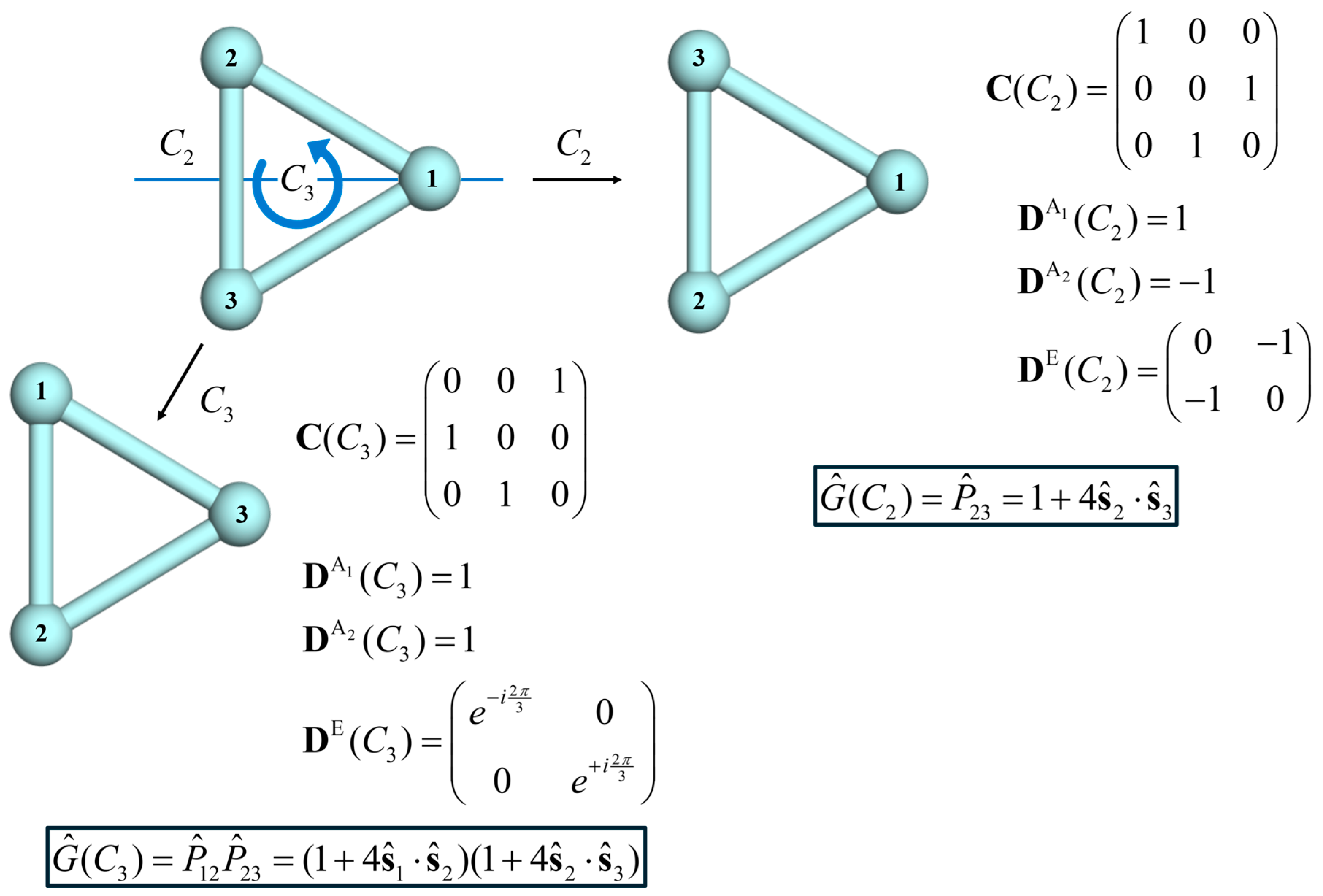
Triangle. An
triangle with three different coupling constants is the smallest system that necessitates matrix diagonalization, because there are two
levels. On the other hand, an isosceles triangle has exchange symmetry,
; with
, the square of the pair spin
is a good quantum number,
. This pair spin is then coupled with
to obtain a total spin multiplet,
yielding the spectrum of Equation (10):
This is the simplest example of Kambe’s method [
33]. In the symmetric triangle, all three couplings are equal, thus Equation (9) becomes
, meaning that all multiplets with the same
S are degenerate [
1].
However, when including biquadratic exchange in the isosceles triangle , remains a symmetry, , but is no longer a good quantum number, because , rendering Kambe’s method inapplicable.
Table 1 lists the subspace dimensions for symmetric triangles up to
, which is the smallest
s that does not permit obtaining the full spectrum in closed form, because there are five
levels. Note that Griffith had already classified terms in triangles, albeit for smaller
s [
34].
Table 1 shows that up to
, there is at most one level in each
sector, so symmetry adaptation suffices to determine the eigenfunctions, and all energies depend linearly on any parameters; phase boundaries in a two- or three-dimensional parameter space would then be straight lines or planes, respectively.
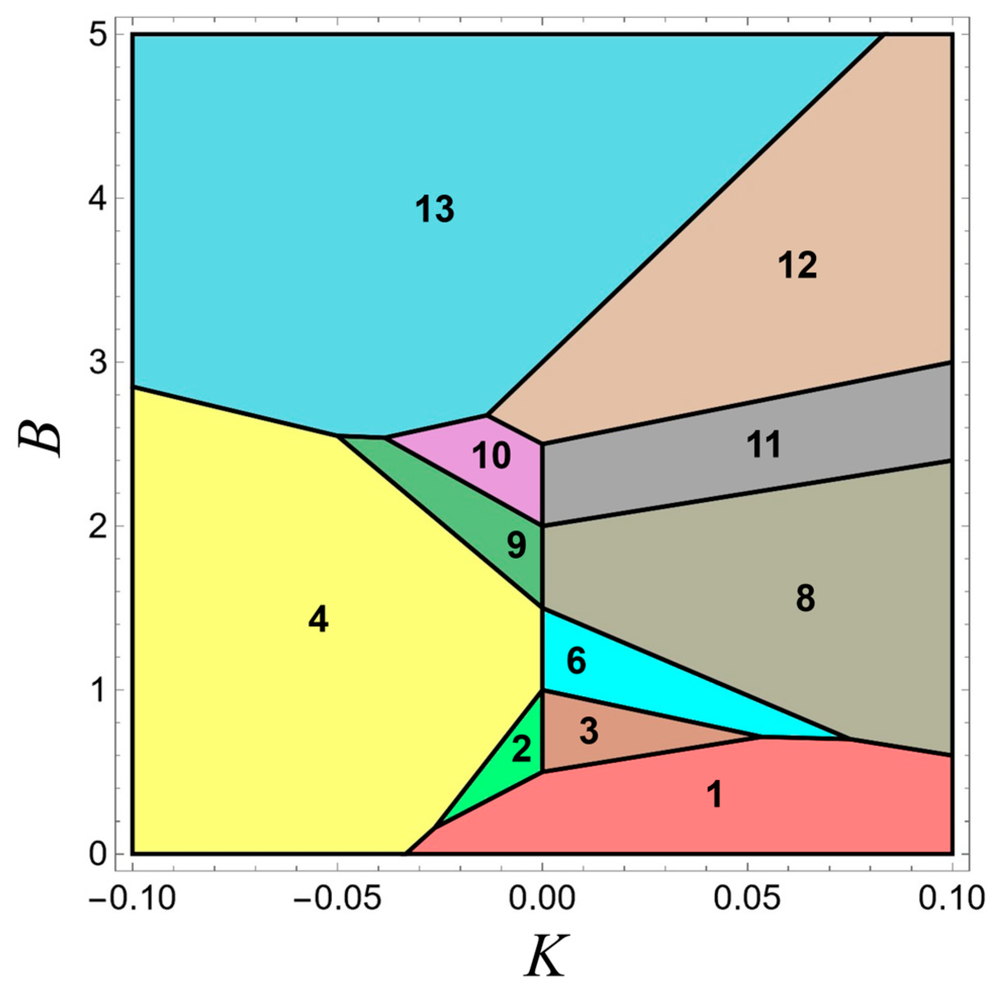
For
and
, we exemplarily collect the full spectra as a function of the biquadratic exchange constant
K in
Table 2 and
Table 3, respectively. (Our Hamiltonian is not exhaustive, e.g., three-center terms, which would occur for
, are ignored.)
The ground states as a function of
K and magnetic field strength
B (Zeeman term,
) are plotted in
Figure 1 and
Figure 2 . These phase diagrams were built on simple analytical conditions, which resemble the ground state conditions in the last columns of
Table 2 and
Table 3, respectively, but also consider the magnetic field strength
B as another independent parameter.
Square. The Heisenberg square, with sites numbered consecutively, is again integrable by Kambe’s method [
1,
35], because
, but
or
do not commute with the biquadratic
. In addition, there exist two independent four-center interactions in the
square (For
, additional four-center (and three-center) interactions involve local rank-2 operators): the frequently discussed cyclic exchange,
and the less common non-cyclic exchange [
19],
Except for
,
and
do not commute with
and
. In other words, biquadratic exchange and multi-center interactions generally prevent trivial spin-coupling solutions. Dimensions of the
sectors are listed in
Table 4, and the spectrum for
as a function of biquadratic and cyclic exchange (
K and
C, respectively) is given in
Table 5.
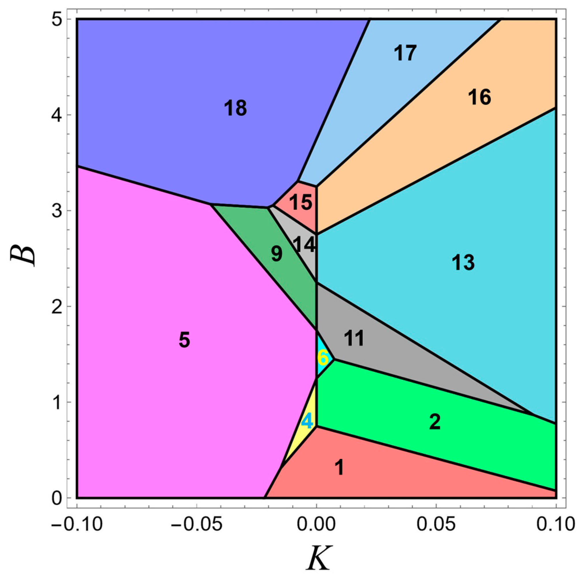
The (
K,
C) ground state criteria are rather complicated and thus not shown here. However, one clear observation, which could not be obtained directly from numerical computations, is that, under the assumption of antiferromagnetic Heisenberg coupling,
, none of the levels 1, 3, 4, 6, 8, 10, 11, 12, 14 or 15 are the ground states for any set (
K,
C). Phase diagrams including a magnetic field, setting either
or
, are shown in
Figure 3.
Polyhedra. Here we shall summarily discuss a few highly symmetric polyhedra. In the tetrahedron, all possible pairs are coupled equally, like in the triangle. Therefore,
is proportional to
,
. Biquadratic exchange again lifts degeneracies because it does not commute with pair spins,
, etc. For
, where a single four-center term is compatible with
symmetry,
the pair spins commute with
, but, as in the case of the square, the respective commutators are non-zero for
. The dimensions of symmetry subspaces are shown in
Table 6. The dimensions for
were previously reported in
Table 4 of Ref. [
36].
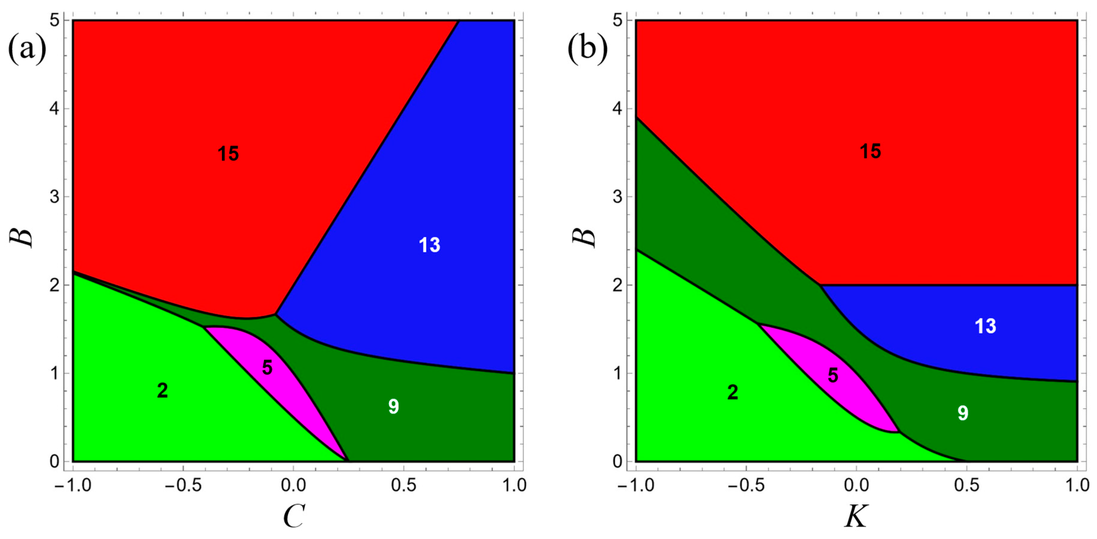
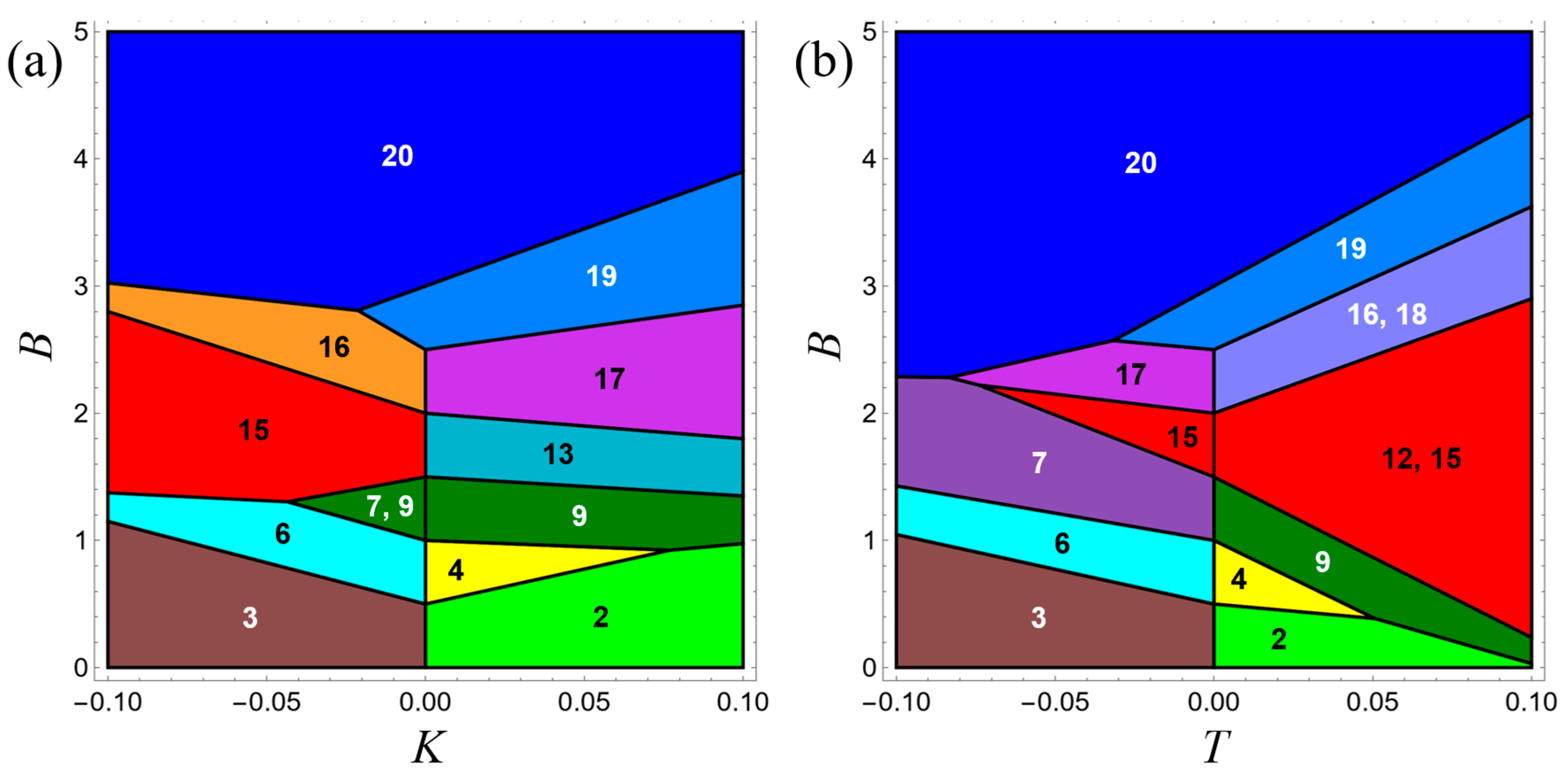
The complete analytical spectrum for the
tetrahedron as a function of
K and
T is exemplarily provided in
Table 7.
For most of the levels, the (
K,
T) criteria for a level to be the lowest-energy state are again quite complex. For
, none of the levels 4, 5, 7, 8, 10, 11, 14, 16, 17, 19 or 20 can be the ground states for any (
K,
T), and 1 is a ground state only on the line
,
.
Figure 4 shows phase diagrams including a magnetic field, setting
or
.
For the octahedron, a formulation of
as in Equation (14),
shows that eigenstates have definite pair spins for diametrically opposite sites. Accidental degeneracies between terms belonging to different
sectors are lifted when incorporating multi-center terms [
19] or biquadratic exchange.
Table 8 shows that the
octahedron is solved directly by spin and PG adaptation, and that the full spectrum can be obtained in closed form for
(not detailed here, due to excessively long expressions for solutions in three- and four-dimensional spaces).
Finally, the Heisenberg cube cannot be solved by Kambe’s method, as it lacks conserved subsystem spins. The dimensions of the symmetry spaces for
, the only
s value for which the cube is fully solvable, are collected in
Table 9. As far as we know, the complete spectrum of
was not derived previously, and we therefore present it in
Table 10. We note accidental degeneracies for
.
4. Summary and Conclusions
While numerical methods are commonly used to investigate spin models of magnetic solids and molecules, small clusters with spatial symmetry allow for analytical diagonalization of the Hamiltonian, and a symbolic representation of spectra or wave functions may provide deeper insights that go beyond mere numerical data. To factor the Hamiltonian into symmetry subspaces and thus enable analytical diagonalization, we provided a simple yet effective approach to adapt the basis to both total spin (using Löwdin’s projector) and point group (PG) symmetry. The construction of PG projectors was extensively discussed. Overall, our procedure for employing spin and PG symmetry to set up a generalized eigenvalue problem in a subspace is not intended to be computationally optimal but designed to be easily followed and implemented. We chose small rings and polyhedra as examples and elucidated how additional interactions (beyond the Heisenberg model) prevent trivial integrability. Our aim was not to compile exhaustive tables but rather to highlight specific results that may be useful for verifying independent implementations of the analytical diagonalization scheme.
It is worth noting that a similar procedure would also be applicable to anisotropic systems. Although a general anisotropic Hamiltonian does not conserve spin,
and
, one can still make use of PG symmetry and apply respective projectors to random states. With anisotropy, most site permutations must be combined with spin rotations to represent symmetries [
24,
26], and this necessitates working with the respective double group for systems with half-integer spin. Analytical solutions for anisotropic models are more severely restricted in terms of system size, because the group is smaller (lacking spin symmetry). Lastly, the present method could also be adapted for use with the Hubbard model, whose additional pseudospin symmetry on a bipartite lattice allows to further block-diagonalize the Hamiltonian [
32,
37]. However, the Hubbard model has itinerant electrons, and, at half-filling, its state space is larger than that of the
Heisenberg model with the same number of sites. Therefore, the limits on system size are stricter.
Note that we leveraged symmetry to factor
H into subspaces for easier diagonalization, but a classification of multiplets in terms of
S and
holds qualitative value too, e.g., for deducing spectroscopic selection rules [
23,
38,
39] or for assessing the momentum-transfer dependencies of inelastic neutron scattering intensities [
23,
39,
40]. Symmetry classifications also aid in analyzing the mixing of multiplets by anisotropic terms [
26,
38].
Analytical solutions can be directly transferred when adding a further spin that has equal couplings to all other sites. The interaction of the original system with such a central site can be handled with Kambe’s method, as detailed in Ref. [
8]. However, the number of non-trivial systems that allow for the closed-form solutions of their entire spectrum is naturally limited by the requirement that neither subspace dimension exceeds four. In some situations, analytical diagonalization could still be used in the smaller spaces of large
S values, which are important to consider for ferromagnetic coupling or in high magnetic fields.

