Review

Biogeochemical Markers to Identify Spatiotemporal Gradients of Phytoplankton across Estuaries

by
Anushka Egoda Gamage
1,2,
Andrew M. Fischer
1,*,
David S. Nichols
3 and
Kim Jye Lee Chang
2
1
Institute for Marine and Antarctic Studies, University of Tasmania, 20 Castray Esplanade, Hobart, TAS 7004, Australia
2
CSIRO Environment, Castray Esplanade, Hobart, TAS 7004, Australia
3
Central Science Laboratory, University of Tasmania, Hobart, TAS 7001, Australia
*
Author to whom correspondence should be addressed.
Coasts 2024, 4(3), 469-481; https://doi.org/10.3390/coasts4030024
Submission received: 6 May 2024 / Revised: 19 June 2024 / Accepted: 20 June 2024 / Published: 1 July 2024

Abstract

:
The spatiotemporal distribution of phytoplankton in estuaries is indicative of processes and transport across the land–ocean aquatic continuum (LOAC). Estuaries, as biogeochemically and physically active systems, process large amounts of nutrients and organic matter influencing the transformation of ecological functions. The transformation of the water column drives variation in phytoplankton composition, biomass, and their spatial distribution. Understanding the dynamics of nutrients and organic matter is challenging, yet it provides a comprehensive insight into phytoplankton spatiotemporal distribution across estuaries. Multiple studies have been conducted to understand the spatiotemporal distribution of phytoplankton. Recently, phytoplankton photosynthetic pigments, fatty acids and stable isotopes have been widely used to identify and quantify phytoplankton distribution. This review highlights the use of biogeochemical markers to identify phytoplankton functional groups. It also assesses the current understanding of patterns in the spatiotemporal distribution of phytoplankton and the impact of physical and environmental factors on their distribution in estuaries and coastal oceans. The review will also gather information from in situ sampling studies to evaluate the current state of knowledge and identify gaps.

1. Introduction

Estuaries are vital interfaces across the land–ocean aquatic continuum (LOAC) [1,2,3,4]. The diverse geomorphology, hydrodynamics and physicochemical properties of these environments, coupled with the high temporal and spatial variability of tides, waves, wind stress, and terrestrial discharge [5,6,7,8], make these challenging environments to study. In addition, since these transitional zones exhibit strong fluctuations in physical and chemical properties, they are highly productive and important ecosystems [1,9,10]. Estuaries act as biological filters and reactors that modify the exchange between terrestrial and coastal ecosystems [4,11], ultimately influencing the coastal marine environment.
The LOAC can be broken down into three components, (1) the terrestrial component and its related contribution to an estuary, (2) the estuarine biological filter/reactor, and (3) the exchange between the estuary and the coastal ocean. The impacts of the terrestrial flow of nutrients and organic matter on estuarine water quality have received more attention over the years [9,12,13,14,15]. Terrestrial discharge into estuarine ecosystems is derived from a wide variety of sources, including surface runoff, groundwater discharge and atmospheric deposition [16,17,18]. Different studies have shown that elevated levels of sediment and particulate nutrients from terrestrial fluxes are largely due to deforestation and agriculture, while dissolved nutrient flux is often associated with agrochemicals [19,20,21]. These inputs affect estuarine biogeochemical factors, which are strongly linked to nutrient cycling and the ecology of associated aquatic biota [22]. Furthermore, fluvial inputs influence stratification, nutrient flux and local circulation patterns altering lower trophic levels and primary productivity by stimulating phytoplankton growth [12,23,24]. In the final component, estuarine outflows carry sediment, nutrients, and organic matter into the coastal ocean. Once there, complex estuarine outflow currents combine with marine waters to create a nutrient-rich distinctive hydrodynamic region in the nearshore environment [25,26]. Thus, outflow characteristics such as organic matter, sediment load, discharge rate, associated physical gradients (e.g., density, temperature, salinity) and hydrodynamic processes can significantly impact and alter the physical, biogeochemical and ecological functions of the coastal ocean.
Primarily, in situ water quality observation approaches have been used to understand the spatiotemporal distribution of phytoplankton within estuarine environments. This review examines the different in situ analytical approaches used to determine phytoplankton dynamics within estuaries and assess the factors that influence their distribution, both physical and biological. Finally, this review will identify integrated methodologies useful to understanding the influence of terrestrial inputs on estuarine systems and the ultimate influence of estuarine exchange on the coastal ocean.

2. Methods

We carried out a literature review using search terms “nutrients and organic matter”, “nutrient dynamics”, “fatty acids”, “pigments” and “stable isotopes”, all combined with estuary phytoplankton. Articles searched in the academic research platforms Google Scholar, Web of Science and University of Tasmania library online database. The search was confined to only journal articles published in international, peer-reviewed journals between 2005 and 2023. However, some articles prior to 2005 were used for comparison against current studies. In situ sampling approaches are categorised into high-performance liquid chromatography to characterize pigments as chemical markers of phytoplankton functional groups, gas chromatography to characterize fatty acid biomarkers of phytoplankton functional groups, and stable isotope signatures to identify the origins of nutrient and organic matter in fluvial fluxes (Figure 1).

3. In Situ Measurements and Phytoplankton Composition

It is widely recognized that pigments and fatty acids are popular methods for quantifying phytoplankton composition and spatiotemporal distribution. Phytoplankton composition analyzed from biomarker pigment and fatty acids data correlates with phytoplankton composition variations across estuaries. Recently stable isotopes (δ13C and δ15N) have been successfully used to determine the source contribution of nutrients and organic matter [27] as fatty acid biomarkers [28]. Therefore, stable isotopes, fatty acid biomarkers and pigments together could be powerful tools to describe phytoplankton distribution patterns and to understand the factors (e.g., nutrients and organic matter) that influence their distribution.

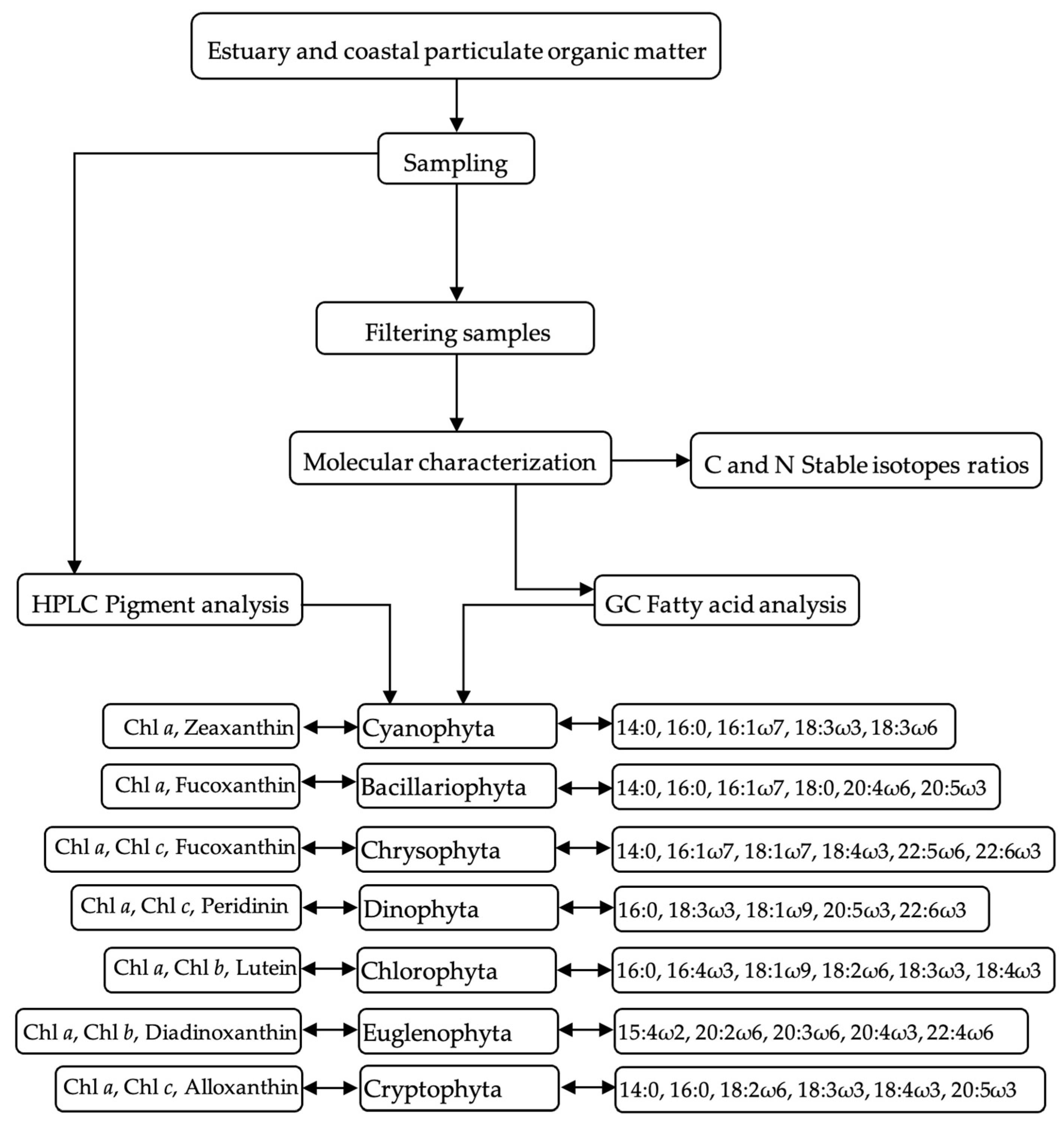
3.1. Fatty Acids to Identify Phytoplankton Functional Groups

Many studies focus on the fatty acids approach to qualitatively characterise phytoplankton community composition and abundance in estuaries [29,30,31,32,33,34]. Several studies have examined fatty acid variations across estuarine systems and fatty acid composition has been used to identify phytoplankton functional groups (Table 1). Studies revealed fatty acids with carbon atoms 16, 18 and 20 as the most abundant in estuarine waters [29,35,36]. Numerous studies have addressed the presence of certain fatty acids across all phytoplankton functional groups, with distinct functional groups being characterized by elevated levels of specific fatty acids. For example, diatoms were distinguished by very high proportions of Eicosapentaenoic acid (EPA); 20:5ω3. The high proportion of Octadecapentaenoic acid (18:5ω3) and Docosahexaenoic acid (DHA), 22:6ω3, suggest the presence of dinoflagellates, and Palmitic acids. Moreover, 16:0 indicates the presence of both diatoms and dinoflagellates [28,36,37,38,39,40,41,42].
In many estuarine phytoplankton studies, diatom biomarker fatty acids were the predominantly sampled fatty acid biomarker, followed by dinoflagellate fatty acids [29,47,48,49]. Fatty acid-based biomarkers are used as a reference to identify estuarine phytoplankton functional groups, yet not all fatty acids are truly taxon-specific, and only a few fatty acids are species-specific [37,50]. Therefore, the applicability of a single fatty acid biomarker can be limited [50]. To compensate for this issue, scientists used an integrated method of fatty acid biomarkers and chemotaxonomic photosynthetic pigment markers [33,43,47,51].

3.2. Pigments to Identify Phytoplankton Groups

According to the literature over 50 phytoplankton pigments have been detected through a high-pressure liquid chromatography (HPLC) method and CHEMTAX program [52]. Reviewing the literature showed that nine major pigment markers have been identified: chlorophyll a, chlorophyll b, chlorophyll c, lutein, zeaxanthin, fucoxanthin, peridinin, diadinoxanthin and ß-carotene, known as biomarkers for several estuarine phytoplankton groups. Chlorophyll a is always the highest in concentration as it is present in all photosynthetic phytoplankton groups [49,53,54]. Many estuarine pigment studies confirmed fucoxanthin (diatoms) as the major light-harvesting pigment followed by peridinin (dinoflagellates) [53,55,56]. A summary of the taxonomic distribution of chlorophyll and carotenoid pigments is presented in Table 2.

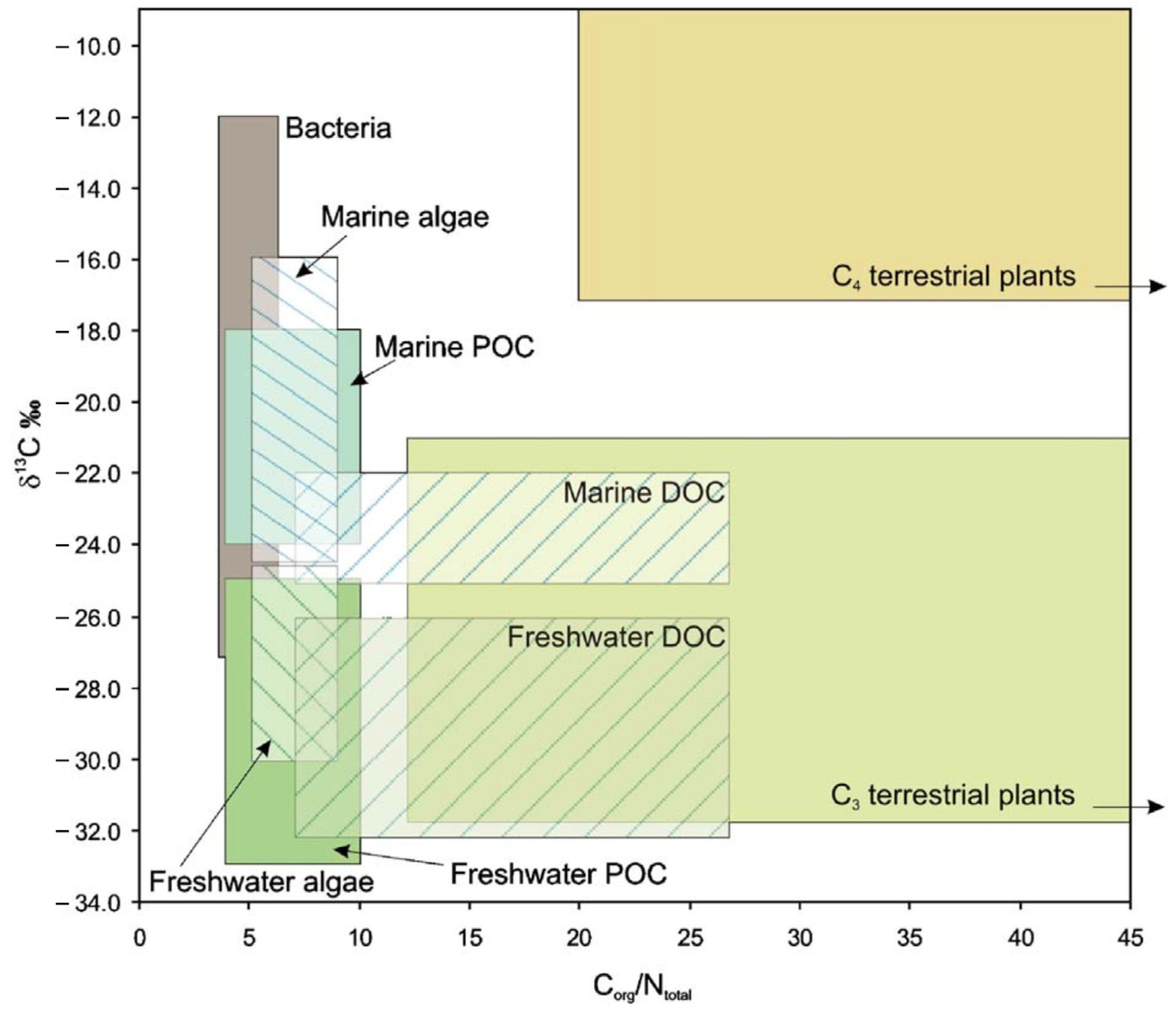
3.3. Stable Isotopes Assess Contribution of Terrestrial Inputs

Aquatic ecosystems process various inputs through many biogeochemical reactions, making tracing the origin of specific elements extremely difficult. To this end, stable isotopes provide valuable information on associated biogeochemical pathways, energy flow between tropic levels and anthropogenic inputs [58,60]. Terrestrial transport of dissolved organic matter and carbon and nitrogen stable isotope ratios (δ13C and δ15N) provides good insight into the source, turnover process and bioavailability of dissolved organic matter [61,62]. The relative abundance of different elemental stable isotopes within compounds may differ significantly [63]. For example, 98.9% of naturally available carbon (C) is represented by the isotope with an atomic mass of 12 (12C), and 1.1% is represented by the isotope with an atomic mass of 13 (13C) [64]. Although isotopic effects are minute in the natural environment [65], subtle changes in heavy and light isotope ratios allow the use of them as “natural dyes” in a wide range of ecological research [66,67].
Prior studies, using δ15N, identified the relative trophic position of organisms. δ13C is widely used for the categorisation of organic carbon sources in the ecosystem, as δ13C values of dissolved organic matter derived from algae and marine phytoplankton are higher (ranging between −12.5 to −25‰) than that derived from the terrestrial origin (ranging between −22 to −31‰), generally largest δ15N values were recorded for saltmarsh and submerged vascular plants (ranged between −2 to 2‰) and the smallest δ15N values were recorded for freshwater marsh plants and estuarine microalgae (ranged between 5–10‰). (Figure 2) [68,69,70,71].

3.4. Combining Pigments, Fatty Acids Biomarkers and Stable Isotopes

Terrestrial discharge carries large quantities of carbon and nitrogen which undergoes rapid removal and decomposition within estuaries [68]. Subsequent studies examined the application of a combined approach of stable isotopes and fatty acids to understand estuary nutrient dynamics. In a Río Negro estuary study, results showed an elevated level of 18:4ω3 and 22:6ω3 due to the influence of dinoflagellates on primary production in the estuary mouth, and higher values of δ13C signatures of organic matter which explained that detritus was from C4 plants [34]. In addition, 20:5ω3, 16:0, chlorophyll a, δ13C and C/N ratios confirmed that upper estuary primary production was driven by diatoms but through tidal export decayed diatoms become autochthones nutrient producers in coastal waters [34]. In both the upper estuary and the estuary mouth, the C/N isotope ratio of 5.7 and 5.8 indicated a strong contribution of phytoplankton to suspended particulate matter. This was confirmed by the presence of fatty acid markers 18:4ω3, 22:6ω3, 20:5ω3, and 16:0 in the same samples. A similar study was performed by [51] in the Scheldt estuary to identify phytoplankton composition and distribution using the combined methods of stable isotopes, fatty acids and pigments. Their study results revealed that diatoms (20:5ω3) and green algae (18:2ω6 and 18:3ω3) were dominant throughout the estuary and could be differentiated by fatty acids and pigments. Terrestrial vegetation or chlorophyte markers 18:2ω6 and 18:3ω3 together with significantly higher isotope values and C/N ratio (approximately −45‰) in the upper estuary suggested that there was little contribution of macrophytes to the upper estuary from terrestrial suspended particulate matter [34]. The study of [51] identified that diatom markers gradually changed with isotopic ratio along the estuary, becoming more positive downstream (δ13C was approximately −35‰ in the upper estuary and −20‰ in the lower estuary) which may have been due to dissolved inorganic carbon isotopes (Figure 3). Both [34,51] revealed that upper estuary bacterial fatty acids and terrestrial origin particulate organic carbon had similar isotope signature values, while estuary mouth bacterial and phytoplankton isotope signature values were similar. These differences in fatty acid profile and isotope signature values were possibly due to upper estuary organic carbon sources originating from sewage and terrestrial matter, while lower estuary organic carbon sources originated from autochthonous phytoplankton. Overall, studies of fatty acid and isotope values C/N ratio revealed the upper estuary’s major organic matter producer was allochthonous origin terrestrial organic matter though, estuary mouth autochthonous phytoplankton were the primary organic matter sources [72,73,74].

3.5. Factors Influencing Phytoplankton Distribution

The spatiotemporal distribution of phytoplankton assemblages and composition across the estuarine system are closely linked to environmental factors such as the seasonal variability of terrestrial fluxes and nutrient availability, light intensity, temperature, salinity, and their interactions [59,75,76]. Among these factors, salinity and availability of nutrients play a major role in the community structure and composition of phytoplankton. Further, the dynamics and composition of estuarine and coastal phytoplankton assemblages are affected by the variability of seasonal and inter-annual terrestrial nutrient loads [47,76] because nutrient and organic matter loading coincide with the tidal influences and freshwater discharge. Several studies have examined the relationship between environmental factors and phytoplankton composition [77,78,79].

3.5.1. Seasonal Variability of Phytoplankton Groups
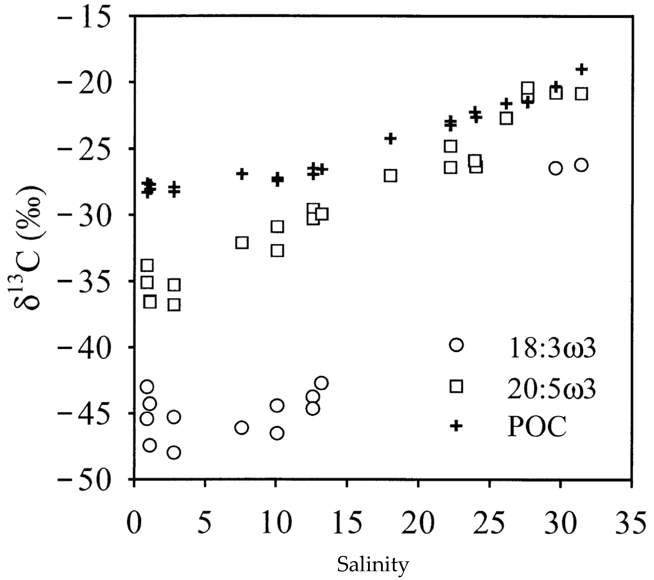
Many studies have shown that diatoms are the dominant phytoplankton group year-round in estuaries [15,80,81]. This is followed by dinoflagellates and chlorophytes [31,32,34,47].
On examining the spatiotemporal dynamics of phytoplankton functional groups within estuaries, [32] revealed that diatoms were the most frequently detected group, around 50% of the total phytoplankton community throughout all four seasons. However, there was a minimum contribution of diatoms during spring and Cyanophyta were more frequent in summer. Despite seasonal differences, dinoflagellates, diatoms, Coccolithophyceae + Pelagophyceae, Eustigmatophyceae, Chlorophyceae + Trebouxiophyceae and cyanophyra phytoplankton groups can be found throughout the year at various concentrations. Similarly, in a pigment analysis study, [49] illustrated the dominance of diatoms throughout the Seomjin River estuary in South Korea. The highest concentration of diatoms was recorded in spring after elevated rain, while dinoflagellate concentrations were low throughout the year. Compared to spring and summer overall phytoplankton composition is markedly low in autumn. Still, in most seasons, diatoms were the dominant phytoplankton group, while cryptophytes dominated only in autumn.
In a recent study by [53] the pigment analysis of the Golden Horn Estuary in Turkey showed that chlorophyll distribution varied across the surface waters of the estuary during the study period. The highest concentration of chlorophyll a was observed during the spring season and the lowest during autumn and winter. When considering their spatial distribution, both diatoms, cryptomonads and dinoflagellates increased towards the upper estuary. Overall, the highest phytoplankton abundance was recorded in May. The concentrations of fucoxanthin and peridinin, which are marker pigments for diatoms and dinoflagellates, were notably higher compared to marker pigments for other phytoplankton groups. The results of [48] were similar to those of [53]. Schnurr et al. [48] revealed a comparatively high biomass of phytoplankton in spring using fatty acids analysis, >50% (µg/mL) of the total biomass represented the diatoms followed by cyanophyta.
Špoljarić et al. [47] compared two estuaries, the subtropical eutrophic Wenchang River Estuary in China and the temperate mesotrophic Krka River Estuary in Croatia to understand the seasonal and spatial factors affecting the estuarine fatty acid composition and phytoplankton distribution. According to the results, the highest phytoplankton biomass was recorded in spring and the lowest occurred during summer; diatoms were the dominant phytoplankton group [47]. Napolitano et al. [29] also identified similar distribution patterns of seasonal phytoplankton blooms and their associated fatty acid biomarkers. The elevated level of chlorophyll a can be attributed to the spring phytoplankton bloom. The substantial levels of diatom fatty acid biomarkers reflected the dominance of diatoms and dinoflagellates within the estuary, which decreased during summer and autumn [29].
Changes in fatty acid and pigment biomarkers composition indicate that phytoplankton biomass from pre-bloom to bloom periods and post-bloom periods provide insight into the effects of seasonal changes in phytoplankton composition. In temperate countries with four distinct seasons, even though nutrient availability is at a maximum level in winter, phytoplankton growth is inhibited by light availability [82]. Further, the higher phytoplankton biomass in the spring season, explained by the increase in snow-melt terrestrial loading alongside high daylight hours and favorable temperature, created suitable environmental conditions to induce phytoplankton photosynthetic activity and increase the biomass, while remaining low in winter due to low nutrients and light availability. Spring with prolonged sunlight and an influx of nutrients, stimulates the growth of phytoplankton, resulting in phytoplankton blooms. However, this rapid growth leads to nutrient depletion, subsequently leading to a decline in biomass and composition and aquatic primary productivity [76]. Maximum sunlight in summer produces perfect conditions for phytoplankton growth, yet diffuse nutrients from spring blooms significantly reduce phytoplankton growth [83]. Limited light and nutrients in autumn phytoplankton growth is gradually declining [55]. However, in tropical countries, phytoplankton growth is limited by nutrients. In the dry season, with low nutrient input, the growth of phytoplankton is inhibited, while the wet season and its high rainfall increase the nutrient flow to produce perfect conditions for increased phytoplankton growth [28,84].

3.5.2. Salinity

When considering spatial distributions, some phytoplankton groups prefer high-saline estuarine mouth areas, and some prefer low-salinity upper estuarine areas. Some groups are distributed throughout the estuary tolerating a wide salinity range [34,49,85,86]. According to the results of [87], dinoflagellates and Chlorophyta groups are prevalent in low salinity areas while diatoms and coccolithophores are mostly present in high salinity areas. This agrees with [51]. Fatty acid composition results showed that Chlorophyta was high in the upper estuary and rapidly declined with the increasing salinity gradients. High salinity areas in the lower estuary contained lower concentrations of Chlorophyta [51,87]. Similar results were shown in [49,53]. Diatoms, represented by the pigment fucoxanthin, and chlorophyll c were relatively high in the upper estuary, yet the dinoflagellate pigments, peridinin, showed opposite distribution patterns to diatoms and were relatively low in concentration in the upper estuary.
In the Schedlt estuary, [43] showed some anomalous patterns of phytoplankton distribution in relation to salinity variations. They observed a considerable decline in phytoplankton biomass along the salinity gradient. Thus, diatoms were the most abundant group in the estuary and their relative abundance increased with increasing salinity (as indicated by the high availability of fucoxanthin, chlorophyll b and FLFA 20:5ω3 at the estuary mouth). Peridinin concentrations for dinoflagellates were only found between 8 to 18 PSU. Chlorophyll b and PLFA 16:3ω3, 16:4ω3, 18:3ω3 representing Chlorophyta showed high abundance in salinity between 0 to 8 PSU and decreased with high salinity with the lowest concentration recorded between 18–28 PSU. Certain fatty acids such as 18:5ω3 and 20:xωx (diatoms) showed an increase in abundance with high salinity gradients. This agrees with the results given by [49] for diatoms (fucoxanthin, δ13C and 20:5ω3) which were higher in high salinity lower estuary areas. Lee et al. [49] revealed that there was a direct response of phytoplankton to nutrient loading associated with the salinity gradient. The study identified that the horizontal distribution of diatoms, dinoflagellates and Cryptophyceae communities in the estuary was influenced by the salinity gradient, which was directly related to nitrogen loading, because of the negative correlation between salinity and nitrogen [49]. According to [49], seasonal and horizontal variations of the phytoplankton community and the influence of environmental factors, particularly salinity and nutrient loading, influenced the abundance and distribution of phytoplankton. Studies revealed distribution patterns of phytoplankton with respect to the salinity gradient across the estuaries. The upper estuary areas with low salinity are characterized by the high prevalence of diatoms, while dinoflagellates are more abundant in the high salinity estuary mouth areas. These findings imply that salinity gradient is a prominent factor affecting the distribution of phytoplankton across estuaries.

3.5.3. Turbidity

Increased sedimentation within the estuary system is often associated with high nutrient availability, low water clarity and high turbidity [88]. Phytoplankton growth is usually higher in lower turbidity as opposed to turbid water with limited light availability [89,90]. Antonio and Richoux [31] showed that most of the fatty acids including fatty acids in the particulate organic matter had negative correlations with estuarine environmental factors such as tidal height, current speed and river discharge which directly influence turbidity. The results of [31] on the influence of the turbidity and tidal cycle on fatty acid composition in the Kowie River estuary, South Africa revealed that phytoplankton biomarker fatty acids were dominant during ebb tide with low turbidity levels throughout the estuary when compared to the flood tide. These results confirmed the study of [32] showing that the estuary’s persistent turbidity level highly influenced low phytoplankton biomass and their spatiotemporal dynamics throughout the year. Suspended sediments reduce light availability which may limit the primary production and consequentially the whole ecosystem [91]. The distribution of chlorophyll concentration negatively correlated with suspended sediment fronts. These results suggest that light limitation due to high turbidity significantly influences the composition and distribution of phytoplankton throughout the estuary.

4. Conclusions

This article reviewed the different methods used to study spatiotemporal distribution and composition of phytoplankton. Overall, water temperature, salinity, turbidity and nutrient concentration are the key factors affecting the spatial distribution of phytoplankton concentrations in coastal and estuarine water. The pattern of seasonal distribution showed winter and spring blooms of diatoms followed by dinoflagellates. The review of the relationship between phytoplankton and environmental factors revealed chlorophyll concentration and total phytoplankton biomass were significantly correlated with salinity, nutrient concentration, temperature and turbidity. However, results from several studies suggest that nutrients and salinity were the major sources of temporal variability in phytoplankton diversity and distribution. Therefore, monitoring estuaries, river discharge dynamics and their physical, chemical, and biological processes is important for understanding the exchange between estuaries and coastal oceans. The impacts of the terrestrial input through the introduction of nutrients and organic matter on estuary phytoplankton have increased in interest over the years. Still, a number of knowledge gaps remain. For example, the use of fatty acids as quantitative phytoplankton biomarkers is limited due to the inadequate availability of phytoplankton fatty acid reference libraries. Most fatty acid-based studies in aquatic systems have been restricted to qualitative estimation of a few available references [32]. Similarly, chlorophylls and carotenoids are commonly used as biomarkers for phytoplankton. However, pigments are not always straightforward because some pigments are generally associated with many phytoplankton taxa and in-situ approaches have their advantages and limitations. These biogeochemical identification methods possess their distinct advantages and limitations. These instrumental methods, coupled with knowledge of taxon-specific pigment composition and fatty acid composition, yield valuable interpretations at the phytoplankton group level. They offer the additional benefit of routine, relatively rapid analysis without requiring extensive algal taxonomy training and with reduced labor compared to microscopy. However, interpretation of data is not always straightforward and is subject to uncertainties linked to biological and environmental sources of variability in pigment and fatty acid composition. For example, the presence of shared marker pigments and fatty acids among several phytoplankton groups makes group identification challenging. Additionally, in situ measurements of water quality parameters are time-consuming, costly, and possess limited spatiotemporal representativeness. They require a standardized sampling procedure and transportation to a laboratory, as well as an experienced analyst to analyze the samples. In addition, the variety of the lab and field measurement methods and instruments involved complicates comparability and reproducibility. Other disadvantages include the need for a large volume of samples and potential quantitative changes during sample storage due to the light sensitivity of pigments. Furthermore, all parts of the process, from water sampling to the final instrumental reading of the fatty acids or pigment content, can be subject to variability. Pigment measurements are now recognized as the standard for calibrating and validating satellite-derived chlorophyll a concentration [92]. Pigment analysis plays a crucial role in validating satellite algorithms for mapping functional types of phytoplankton. Satellites enable sampling over much larger spatial scales than feasible with in situ sampling and at frequencies that are impossible to match by any other sampling procedure. Earth-observing ocean color satellites now provide continuous, high-frequency daily measurements over large oceanic regions to help use data for coastal water analysis and forecasting. However, cloud cover is the most fundamental limitation to ocean color observation as it masks the sea surface. Since the satellite signal originates in the surface layer, it usually provides near-surface chlorophyll levels, and obtaining sub-surface chlorophyll readings is not feasible. Finally, it is clear that relying on any one method in isolation would result in characterizing phytoplankton groups that may not be entirely complete or unambiguous. Therefore, approaches integrating data from various methodologies provide more accurate and comprehensive assessments.
Improving technology and analytical advancements provide a robust framework for studying and assessing estuarine exchange through phytoplankton biomass and their spatiotemporal distribution. To obtain a comprehensive understanding of phytoplankton dynamics and understand the coastal estuary exchange and its influence on phytoplankton spatiotemporal distribution, it is often helpful to use a combination of different methods. To this end, integrating multiple approaches is likely to provide more comprehensive information across multiple temporal and spatial scales. Integrated satellite remote sensing and hydrodynamic modelling can be used to examine larger spatial areas over time, which may be difficult to achieve with only field observations.

Author Contributions

Conceptualization, writing—original draft preparation, A.E.G.; writing—review and editing, visualization, A.E.G. and A.M.F.; supervision, A.M.F., D.S.N. and K.J.L.C. All authors have read and agreed to the published version of the manuscript.

Funding

This research was funded by University of Tasmania CoSE Research Training Program (RTP) Stipend and the CSIRO Top-Up Scholarship.

Acknowledgments

This research was supported by University of Tasmania CoSE Research Training Program (RTP) Stipend and the CSIRO Top-Up Scholarship. The authors are grateful to the NRM North, Tamar Estuary and Esk Rivers program team for providing data and assisting in sample collection throughout the research. Additionally, we would like to express our appreciation to the three anonymous reviewers whose comments significantly improved the paper.

Conflicts of Interest

The authors declare no conflicts of interest.

References

  1. Cloern, J.E.; Foster, S.Q.; Kleckner, A.E. Phytoplankton primary production in the world’s estuarine-coastal ecosystems. Biogeosciences 2014, 11, 2477–2501. [Google Scholar] [CrossRef]
  2. Geyer, W.R.; Hill, P.S.; Kineke, G.C. The transport, transformation and dispersal of sediment by buoyant coastal flows. Cont. Shelf Res. 2004, 24, 927–949. [Google Scholar] [CrossRef]
  3. Conroy, T.; Sutherland, D.A.; Ralston, D.K. Estuarine Exchange Flow Variability in a Seasonal, Segmented Estuary. J. Phys. Oceanogr. 2020, 50, 595–613. [Google Scholar] [CrossRef]
  4. Humborg, C.; Danielsson, Å.; Sjöberg, B.; Green, M. Nutrient land–sea fluxes in oligothrophic and pristine estuaries of the Gulf of Bothnia, Baltic Sea. Estuar. Coast. Shelf Sci. 2003, 56, 781–793. [Google Scholar] [CrossRef]
  5. Inoue, M.; Wiseman, W.J. Transport, Mixing and Stirring Processes in a Louisiana Estuary: A Model Study. Estuar. Coast. Shelf Sci. 2000, 50, 449–466. [Google Scholar] [CrossRef]
  6. Kitheka, J.U.; Obiero, M.; Nthenge, P. River discharge, sediment transport and exchange in the Tana Estuary, Kenya. Estuar. Coast. Shelf Sci. 2005, 63, 455–468. [Google Scholar] [CrossRef]
  7. Osadchiev, A.; Medvedev, I.; Shchuka, S.; Kulikov, M.; Spivak, E.; Pisareva, M.; Semiletov, I. Influence of estuarine tidal mixing on structure and spatial scales of large river plumes. Ocean Sci. 2020, 16, 781–798. [Google Scholar] [CrossRef]
  8. Wei, X.; Kumar, M.; Schuttelaars, H.M. Three-Dimensional Salt Dynamics in Well-Mixed Estuaries: Influence of Estuarine Convergence, Coriolis, and Bathymetry. J. Phys. Oceanogr. 2017, 47, 1843–1871. [Google Scholar] [CrossRef]
  9. Fisher, T.R.; Harding, L.W., Jr.; Stanley, D.W.; Ward, L.G. Phytoplankton, nutrients, and turbidity in the Chesapeake, Delaware, and Hudson estuaries. Estuar. Coast. Shelf Sci. 1988, 27, 61–93. [Google Scholar] [CrossRef]
  10. Chen, C.Y.; Buckman, K.L.; Shaw, A.; Curtis, A.; Taylor, M.; Montesdeoca, M.; Driscoll, C. The influence of nutrient loading on methylmercury availability in Long Island estuaries. Environ. Pollut. 2021, 268. [Google Scholar] [CrossRef]
  11. Sanders, T.; Schöl, A.; Dähnke, K. Hot Spots of Nitrification in the Elbe Estuary and Their Impact on Nitrate Regeneration. Estuaries Coasts 2017, 41, 128–138. [Google Scholar] [CrossRef]
  12. McGovern, M.; Pavlov, A.K.; Deininger, A.; Granskog, M.A.; Leu, E.; Søreide, J.E.; Poste, A.E. Terrestrial Inputs Drive Seasonality in Organic Matter and Nutrient Biogeochemistry in a High Arctic Fjord System (Isfjorden, Svalbard). Front. Mar. Sci. 2020, 7. [Google Scholar] [CrossRef]
  13. Reese, L.; Gräwe, U.; Klingbeil, K.; Li, X.; Lorenz, M.; Burchard, H. Local Mixing Determines Spatial Structure of Diahaline Exchange Flow in a Mesotidal Estuary: A Study of Extreme Runoff Conditions. J. Phys. Oceanogr. 2024, 54, 3–27. [Google Scholar] [CrossRef]
  14. Stefánsson, U.; Richards, F.A. Processes contributing to the nutrient distribution off the columbia river and strait of juan de fuca 1. Limnol. Oceanogr. 1963, 8, 394–410. [Google Scholar] [CrossRef]
  15. Ouyang, W.; Wang, R.; Ji, K.; Liu, X.; Geng, F.; Hao, X.; Lin, C. Phytoplankton biomass dynamics with diffuse terrestrial nutrients pollution discharge into bay. Chemosphere 2023, 313, 137674. [Google Scholar] [CrossRef]
  16. Adyasari, D.; Oehler, T.; Afiati, N.; Moosdorf, N. Groundwater nutrient inputs into an urbanized tropical estuary system in Indonesia. Sci. Total Environ. 2018, 627, 1066–1079. [Google Scholar] [CrossRef]
  17. Kaul, L.W.; Froelich, P.N. Modeling estuarine nutrient geochemistry in a simple system. Geochim. Cosmochim. Acta 1984, 48, 1417–1433. [Google Scholar] [CrossRef]
  18. Seitzinger, S.P.; Sanders, R.W. Atmospheric inputs of dissolved organic nitrogen stimulate estuarine bacteria and phytoplankton. Limnol. Oceanogr. 1999, 44, 721–730. [Google Scholar] [CrossRef]
  19. Vendramini, J.; Silveira, M.; Dubeux, J., Jr.; Sollenberger, L. Environmental impacts and nutrient recycling on pastures grazed by cattle. Rev. Bras. Zootec. 2007, 36, 139–149. [Google Scholar] [CrossRef]
  20. Bull, E.; Cunha, C.d.L.; Scudelari, A. Water quality impact from shrimp farming effluents in a tropical estuary. Water Sci. Technol. 2021, 83, 123–136. [Google Scholar] [CrossRef]
  21. Conrad, S.R.; Santos, I.R.; White, S.; Sanders, C.J. Nutrient and Trace Metal Fluxes into Estuarine Sediments Linked to Historical and Expanding Agricultural Activity (Hearnes Lake, Australia). Estuaries Coasts 2019, 42, 944–957. [Google Scholar] [CrossRef]
  22. Bukaveckas, P.A.; Isenberg, W. Loading, transformation, and retention of nitrogen and phosphorus in the tidal freshwater James River (Virginia). Estuaries Coasts 2013, 36, 1219–1236. [Google Scholar] [CrossRef]
  23. Paczkowska, J.; Brugel, S.; Rowe, O.; Lefébure, R.; Brutemark, A.; Andersson, A. Response of Coastal Phytoplankton to High Inflows of Terrestrial Matter. Front. Mar. Sci. 2020, 7. [Google Scholar] [CrossRef]
  24. Geider, R.J.; Delucia, E.H.; Falkowski, P.G.; Finzi, A.C.; Grime, J.P.; Grace, J.; Kana, T.M.; La Roche, J.; Long, S.P.; Osborne, B.A.; et al. Primary productivity of planet earth: Biological determinants and physical constraints in terrestrial and aquatic habitats. Glob. Chang. Biol. 2001, 7, 849–882. [Google Scholar] [CrossRef]
  25. Dzwonkowski, B.; Greer, A.T.; Briseño-Avena, C.; Krause, J.W.; Soto, I.M.; Hernandez, F.J.; Deary, A.L.; Wiggert, J.D.; Joung, D.; Fitzpatrick, P.J.; et al. Estuarine influence on biogeochemical properties of the Alabama shelf during the fall season. Cont. Shelf Res. 2017, 140, 96–109. [Google Scholar] [CrossRef]
  26. Davis, K.A.; Banas, N.S.; Giddings, S.N.; Siedlecki, S.A.; MacCready, P.; Lessard, E.J.; Kudela, R.M.; Hickey, B.M. Estuary-enhanced upwelling of marine nutrients fuels coastal productivity in the U.S. Pacific Northwest. J. Geophys. Res. Ocean. 2014, 119, 8778–8799. [Google Scholar] [CrossRef]
  27. Maier, G.O.; Toft, J.D.; Simenstad, C.A. Variability in Isotopic (δ13C, δ15N, δ34S) Composition of Organic Matter Contributing to Detritus-Based Food Webs of the Columbia River Estuary. Northwest Sci. 2011, 85, 41–54. [Google Scholar] [CrossRef]
  28. Gardade, L.; Khandeparker, L.; Desai, D.V.; Atchuthan, P.; Anil, A.C. Fatty acids as indicators of sediment organic matter dynamics in a monsoon-influenced tropical estuary. Ecol. Indic. 2021, 130, 108014. [Google Scholar] [CrossRef]
  29. Napolitano, G.E.; Pollero, R.J.; Gayoso, A.M.; Macdonald, B.A.; Thompson, R.J. Fatty acids as trophic markers of phytoplankton blooms in the Bahia Blanca estuary (Buenos Aires, Argentina) and in Trinity Bay (Newfoundland, Canada). Biochem. Syst. Ecol. 1997, 25, 739–755. [Google Scholar] [CrossRef]
  30. Cañavate, J.-P.; van Bergeijk, S.; González-Ortegón, E.; Vílas, C. Contrasting fatty acids with other indicators to assess nutritional status of suspended particulate organic matter in a turbid estuary. Estuar. Coast. Shelf Sci. 2021, 254, 107329. [Google Scholar] [CrossRef]
  31. Antonio, E.S.; Richoux, N.B. Tide-Induced Variations in the Fatty Acid Composition of Estuarine Particulate Organic Matter. Estuaries Coasts 2015, 39, 1072–1083. [Google Scholar] [CrossRef]
  32. Cañavate, J.-P.; van Bergeijk, S.; Giráldez, I.; González-Ortegón, E.; Vílas, C. Fatty Acids to Quantify Phytoplankton Functional Groups and Their Spatiotemporal Dynamics in a Highly Turbid Estuary. Estuaries Coasts 2019, 42, 1971–1990. [Google Scholar] [CrossRef]
  33. Fischer, A.M.; Ryan, J.P.; Levesque, C.; Welschmeyer, N. Characterizing estuarine plume discharge into the coastal ocean using fatty acid biomarkers and pigment analysis. Mar. Environ. Res. 2014, 99, 106–116. [Google Scholar] [CrossRef]
  34. Kopprio, G.A.; Dutto, M.S.; Garzón Cardona, J.E.; Gärdes, A.; Lara, R.J.; Graeve, M. Biogeochemical markers across a pollution gradient in a Patagonian estuary: A multidimensional approach of fatty acids and stable isotopes. Mar. Pollut. Bull. 2018, 137, 617–626. [Google Scholar] [CrossRef]
  35. Ruiz-Ruiz, P.A.; Contreras, S.; Urzúa, Á.; Quiroga, E.; Rebolledo, L. Fatty acid biomarkers in three species inhabiting a high latitude Patagonian fjord (Yendegaia Fjord, Chile). Polar Biol. 2021, 44, 147–162. [Google Scholar] [CrossRef]
  36. Pang, S.Y.; Suratman, S.; Fadzil, M.F.; Tan, H.S.; Le, D.Q.; Mostapa, R.; Simoneit, B.R.T.; Tahir, N.M. Lipid biomarkers, stable C and N isotope ratios coupled with multivariate statistics as sources indicators in coastal sediments of Brunei Bay, Southern South China Sea. Reg. Stud. Mar. Sci. 2021, 48, 11. [Google Scholar] [CrossRef]
  37. Chuecas, L.; Riley, J.P. Component Fatty Acids of the Total Lipids of Some Marine Phytoplankton. J. Mar. Biol. Assoc. UK 1969, 49, 97–116. [Google Scholar] [CrossRef]
  38. DeMort, C.L.; Lowry, R.; Tinsley, I.; Phinney, H. The biochemical analysis of some estuarine phytoplankton species. i. fatty acid composition 1 2. J. Phycol. 1972, 8, 211–216. [Google Scholar] [CrossRef]
  39. Bosley, K.M.; Copeman, L.A.; Dumbauld, B.R.; Bosley, K.L. Identification of burrowing shrimp food sources along an estuarine gradient using fatty acid analysis and stable isotope ratios. Estuaries Coasts 2017, 40, 1113–1130. [Google Scholar] [CrossRef]
  40. Richoux, N.B.; Froneman, P.W. Trophic ecology of dominant zooplankton and macrofauna in a temperate, oligotrophic South African estuary: A fatty acid approach. Mar. Ecol. Prog. Ser. 2008, 357, 121–137. [Google Scholar] [CrossRef]
  41. Sofía Dutto, M.; Kopprio, G.A.; Hoffmeyer, M.S.; Alonso, T.S.; Graeve, M.; Kattner, G. Planktonic trophic interactions in a human-impacted estuary of Argentina: A fatty acid marker approach. J. Plankton Res. 2014, 36, 776–787. [Google Scholar] [CrossRef]
  42. Kelly, J.R.; Scheibling, R.E. Fatty acids as dietary tracers in benthic food webs. Mar. Ecol. Prog. Ser. 2012, 446, 1–22. [Google Scholar] [CrossRef]
  43. Dijkman, N.A.; Kromkamp, J.C. Phospholipid-derived fatty acids as chemotaxonomic markers for phytoplankton: Application for inferring phytoplankton composition. Mar. Ecol. Prog. Ser. 2006, 324, 113–125. [Google Scholar] [CrossRef]
  44. Jónasdóttir, S.H. Fatty acid profiles and production in marine phytoplankton. Mar. Drugs 2019, 17, 151. [Google Scholar] [CrossRef]
  45. Shilla, D.; Routh, J. Using biochemical and isotopic tracers to characterise organic matter sources and their incorporation into estuarine food webs (Rufiji delta, Tanzania). Chem. Ecol. 2017, 33, 893–917. [Google Scholar] [CrossRef]
  46. Taipale, S.J.; Peltomaa, E.; Hiltunen, M.; Jones, R.I.; Hahn, M.W.; Biasi, C.; Brett, M.T. Inferring phytoplankton, terrestrial plant and bacteria bulk δ¹³C values from compound specific analyses of lipids and fatty acids. PLoS ONE 2015, 10, e0133974. [Google Scholar] [CrossRef]
  47. Špoljarić, I.V.; Novak, T.; Gašparović, B.; Kazazić, S.P.; Čanković, M.; Ljubešić, Z.; Hrustić, E.; Mlakar, M.; Du, J.; Zhang, R. Impact of environmental conditions on phospholipid fatty acid composition: Implications from two contrasting estuaries. Aquat. Ecol. 2021, 55, 1–20. [Google Scholar] [CrossRef]
  48. Schnurr, P.J.; Drever, M.C.; Kling, H.J.; Elner, R.W.; Arts, M.T. Seasonal changes in fatty acid composition of estuarine intertidal biofilm: Implications for western sandpiper migration. Estuar. Coast. Shelf Sci. 2019, 224, 94–107. [Google Scholar] [CrossRef]
  49. Lee, M.; Won, N.-I.; Baek, S.H. Comparison of HPLC Pigment Analysis and Microscopy in Phytoplankton Assessment in the Seomjin River Estuary, Korea. Sustainability 2020, 12, 1675. [Google Scholar] [CrossRef]
  50. Strandberg, U.; Taipale, S.J.; Hiltunen, M.; Galloway, A.W.E.; Brett, M.T.; Kankaala, P. Inferring phytoplankton community composition with a fatty acid mixing model. Ecosphere 2015, 6, art16. [Google Scholar] [CrossRef]
  51. Boschker, H.T.S.; Kromkamp, J.C.; Middelburg, J.J. Biomarker and carbon isotopic constraints on bacterial and algal community structure and functioning in a turbid, tidal estuary. Limnol. Oceanogr. 2005, 50, 70–80. [Google Scholar] [CrossRef]
  52. Wright, S.W.; Jeffrey, S. Pigment Markers for Phytoplankton Production. In Marine Organic Matter: Biomarkers, Isotopes and DNA; Springer: Berlin/Heidelberg, Germany, 2006; pp. 71–104. [Google Scholar]
  53. Dursun, F.; Tas, S.; Ediger, D. Assessment of phytoplankton group composition in the Golden Horn Estuary (Sea of Marmara, Turkey) determined with pigments measured by HPLC-CHEMTAX analyses and microscopy. J. Mar. Biol. Assoc. UK 2021, 101, 649–665. [Google Scholar] [CrossRef]
  54. Damar, A.; Colijn, F.; Hesse, K.-J.; Kurniawan, F. Coastal Phytoplankton Pigments Composition in Three Tropical Estuaries of Indonesia. J. Mar. Sci. Eng. 2020, 8, 311. [Google Scholar] [CrossRef]
  55. Chai, C.; Jiang, T.; Cen, J.; Ge, W.; Lu, S. Phytoplankton pigments and functional community structure in relation to environmental factors in the Pearl River Estuary. Oceanologia 2016, 58, 201–211. [Google Scholar] [CrossRef]
  56. Laza-Martinez, A.; Seoane, S.; Zapata, M.; Orive, E. Phytoplankton pigment patterns in a temperate estuary: From unialgal cultures to natural assemblages. J. Plankton Res. 2007, 29, 913–929. [Google Scholar] [CrossRef]
  57. Wright, S.; Jeffrey, S.; Mantoura, R. Phytoplankton Pigments in Oceanography: Guidelines to Modern Methods; Unesco Pub.: Paris, France, 2005. [Google Scholar]
  58. Gibb, S.W.; Cummings, D.G.; Irigoien, X.; Barlow, R.G.; Fauzi, R.; Mantoura, C. Phytoplankton pigment chemotaxonomy of the northeastern Atlantic. Deep Sea Res. Part II Top. Stud. Oceanogr. 2001, 48, 795–823. [Google Scholar] [CrossRef]
  59. Vijayan, A.K.; Reddy, B.B.; Sudheesh, V.; Marathe, P.H.; Nampoothiri, V.N.; Harikrishnachari, N.V.; Kavya, P.; Gupta, G.V.M.; Ramanamurthy, M.V. Phytoplankton community structure in a contrasting physico-chemical regime along the eastern Arabian Sea during the winter monsoon. J. Mar. Syst. 2021, 215. [Google Scholar] [CrossRef]
  60. Schmidt, H.-L.; Robins, R.J.; Werner, R.A. Multi-factorial in vivo stable isotope fractionation: Causes, correlations, consequences and applications. Isot. Environ. Health Stud. 2015, 51, 155–199. [Google Scholar] [CrossRef] [PubMed]
  61. Benner, R. What happens to terrestrial organic matter in the ocean? Mar. Chem. 2004, 92, 307–310. [Google Scholar] [CrossRef]
  62. Botto, F.; Gaitán, E.; Mianzan, H.; Acha, M.; Giberto, D.; Schiariti, A.; Iribarne, O. Origin of resources and trophic pathways in a large SW Atlantic estuary: An evaluation using stable isotopes. Estuar. Coast. Shelf Sci. 2011, 92, 70–77. [Google Scholar] [CrossRef]
  63. Hoefs, J. Stable Isotope Geochemistry; Springer: Berlin, Germany, 1997. [Google Scholar]
  64. De Laeter, J.R.; Böhlke, J.K.; De Bievre, P.; Hidaka, H.; Peiser, H.; Rosman, K.; Taylor, P. Atomic weights of the elements. Review 2000 (IUPAC Technical Report). Pure Appl. Chem. 2003, 75, 683–800. [Google Scholar] [CrossRef]
  65. Berg, T.; Strand, D.H. 13C labelled internal standards—A solution to minimize ion suppression effects in liquid chromatography–tandem mass spectrometry analyses of drugs in biological samples? J. Chromatogr. A 2011, 1218, 9366–9374. [Google Scholar] [CrossRef] [PubMed]
  66. Robinson, D. δ15N as an integrator of the nitrogen cycle. Trends Ecol. Evol. 2001, 16, 153–162. [Google Scholar] [CrossRef] [PubMed]
  67. Boschker, H.; Middelburg, J. Stable isotopes and biomarkers in microbial ecology. FEMS Microbiol. Ecol. 2002, 40, 85–95. [Google Scholar] [CrossRef] [PubMed]
  68. Ye, F.; Guo, W.; Wei, G.; Jia, G. The Sources and Transformations of Dissolved Organic Matter in the Pearl River Estuary, China, as Revealed by Stable Isotopes. J. Geophys. Res. Ocean. 2018, 123, 6893–6908. [Google Scholar] [CrossRef]
  69. Alfaro, A.C.; Thomas, F.; Sergent, L.; Duxbury, M. Identification of trophic interactions within an estuarine food web (northern New Zealand) using fatty acid biomarkers and stable isotopes. Estuar. Coast. Shelf Sci. 2006, 70, 271–286. [Google Scholar] [CrossRef]
  70. Cloern, J.E.; Canuel, E.A.; Harris, D. Stable carbon and nitrogen isotope composition of aquatic and terrestrial plants of the San Francisco Bay estuarine system. Limnol. Oceanogr. 2002, 47, 713–729. [Google Scholar] [CrossRef]
  71. Lamb, A.L.; Wilson, G.P.; Leng, M.J. A review of coastal palaeoclimate and relative sea-level reconstructions using δ13C and C/N ratios in organic material. Earth-Sci. Rev. 2006, 75, 29–57. [Google Scholar] [CrossRef]
  72. Bergamino, L.; Dalu, T.; Richoux, N.B. Evidence of spatial and temporal changes in sources of organic matter in estuarine sediments: Stable isotope and fatty acid analyses. Hydrobiologia 2014, 732, 133–145. [Google Scholar] [CrossRef]
  73. Hu, J.; Peng, P.A.; Jia, G.; Mai, B.; Zhang, G. Distribution and sources of organic carbon, nitrogen and their isotopes in sediments of the subtropical Pearl River estuary and adjacent shelf, Southern China. Mar. Chem. 2006, 98, 274–285. [Google Scholar] [CrossRef]
  74. McIntosh, H.A.; McNichol, A.P.; Xu, L.; Canuel, E.A. Source—Age dynamics of estuarine particulate organic matter using fatty acid δ13C and Δ14C composition. Limnol. Oceanogr. 2015, 60, 611–628. [Google Scholar] [CrossRef]
  75. Wissel, B.; Gaçe, A.; Fry, B. Tracing river influences on phytoplankton dynamics in two louisiana estuaries. Ecology 2005, 86, 2751–2762. [Google Scholar] [CrossRef]
  76. Bargu, S.; Justic, D.; White, J.R.; Lane, R.; Day, J.; Paerl, H.; Raynie, R. Mississippi River diversions and phytoplankton dynamics in deltaic Gulf of Mexico estuaries: A review. Estuar. Coast. Shelf Sci. 2019, 221, 39–52. [Google Scholar] [CrossRef]
  77. Pulina, S.; Satta, C.T.; Padedda, B.M.; Sechi, N.; Lugliè, A. Seasonal variations of phytoplankton size structure in relation to environmental variables in three Mediterranean shallow coastal lagoons. Estuar. Coast. Shelf Sci. 2018, 212, 95–104. [Google Scholar] [CrossRef]
  78. Dijkstra, Y.M.; Chant, R.J.; Reinfelder, J.R. Factors controlling seasonal phytoplankton dynamics in the Delaware River Estuary: An idealized model study. Estuaries Coasts 2019, 42, 1839–1857. [Google Scholar] [CrossRef]
  79. Liu, B.; D’Sa, E.J.; Maiti, K.; Rivera-Monroy, V.H.; Xue, Z. Biogeographical trends in phytoplankton community size structure using adaptive sentinel 3-OLCI chlorophyll a and spectral empirical orthogonal functions in the estuarine-shelf waters of the northern Gulf of Mexico. Remote Sens. Environ. 2021, 252, 112154. [Google Scholar] [CrossRef]
  80. Carstensen, J.; Klais, R.; Cloern, J.E. Phytoplankton blooms in estuarine and coastal waters: Seasonal patterns and key species. Estuar. Coast. Shelf Sci. 2015, 162, 98–109. [Google Scholar] [CrossRef]
  81. Ge, J.; Torres, R.; Chen, C.; Liu, J.; Xu, Y.; Bellerby, R.; Shen, F.; Bruggeman, J.; Ding, P. Influence of suspended sediment front on nutrients and phytoplankton dynamics off the Changjiang Estuary: A FVCOM-ERSEM coupled model experiment. J. Mar. Syst. 2020, 204, 103292. [Google Scholar] [CrossRef]
  82. Labry, C.; Herbland, A.; Delmas, D.; Laborde, P.; Lazure, P.; Froidefond, J.; Jegou, A.-M.; Sautour, B. Initiation of winter phytoplankton blooms within the Gironde plume waters in the Bay of Biscay. Mar. Ecol. Prog. Ser. 2001, 212, 117–130. [Google Scholar] [CrossRef]
  83. Moschonas, G.; Gowen, R.J.; Paterson, R.F.; Mitchell, E.; Stewart, B.M.; McNeill, S.; Glibert, P.M.; Davidson, K. Nitrogen dynamics and phytoplankton community structure: The role of organic nutrients. Biogeochemistry 2017, 134, 125–145. [Google Scholar] [CrossRef]
  84. Soria-Píriz, S.; García-Robledo, E.; Papaspyrou, S.; Aguilar, V.; Seguro, I.; Acuña, J.; Morales, Á.; Corzo, A. Size fractionated phytoplankton biomass and net metabolism along a tropical estuarine gradient. Limnol. Oceanogr. 2017, 62, S309–S326. [Google Scholar] [CrossRef]
  85. Jiang, Z.; Chen, J.; Zhou, F.; Shou, L.; Chen, Q.; Tao, B.; Yan, X.; Wang, K. Controlling factors of summer phytoplankton community in the Changjiang (Yangtze River) Estuary and adjacent East China Sea shelf. Cont. Shelf Res. 2015, 101, 71–84. [Google Scholar] [CrossRef]
  86. Cañavate, J.-P.; Fernández-Díaz, C. Salinity induces unique changes in lipid classes and fatty acids of the estuarine haptophyte Diacronema vlkianum. Eur. J. Phycol. 2021, 57, 297–317. [Google Scholar] [CrossRef]
  87. Viličić, D.; Terzić, S.; Ahel, M.; Burić, Z.; Jasprica, N.; Carić, M.; Mihalić, K.C.; Olujić, G. Phytoplankton abundance and pigment biomarkers in the oligotrophic, eastern Adriatic estuary. Environ. Monit. Assess. 2008, 142, 199–218. [Google Scholar] [CrossRef] [PubMed]
  88. Lovelock, C.E.; Feller, I.C.; Ellis, J.; Schwarz, A.M.; Hancock, N.; Nichols, P.; Sorrell, B. Mangrove growth in New Zealand estuaries: The role of nutrient enrichment at sites with contrasting rates of sedimentation. Oecologia 2007, 153, 633–641. [Google Scholar] [CrossRef] [PubMed]
  89. Lancelot, C.; Muylaert, K. 7.02 Trends in estuarine phytoplankton ecology. In Treatise on Estuarine and Coastal Science; Academic Press: Waltham, MA, USA, 2011; pp. 5–15. [Google Scholar]
  90. O’Meara, T.A.; Hillman, J.R.; Thrush, S.F. Rising tides, cumulative impacts and cascading changes to estuarine ecosystem functions. Sci. Rep. 2017, 7, 10218. [Google Scholar] [CrossRef] [PubMed]
  91. Wang, Y.; Wu, H.; Lin, J.; Zhu, J.; Zhang, W.; Li, C. Phytoplankton Blooms off a High Turbidity Estuary: A Case Study in the Changjiang River Estuary. J. Geophys. Res. Ocean. 2019, 124, 8036–8059. [Google Scholar] [CrossRef]
  92. Moisan, T.A.; Rufty, K.M.; Moisan, J.R.; Linkswiler, M.A. Satellite Observations of Phytoplankton Functional Type Spatial Distributions, Phenology, Diversity, and Ecotones. Front. Mar. Sci. 2017, 4. [Google Scholar] [CrossRef]
Figure 1. Conceptual model illustrating the process of in-situ water analysis.
Coasts 04 00024 g001
Figure 2. Carbon stable isotope (δ13C) values and carbon to nitrogen (C:N) ratios for organic inputs in coastal environments. Reproduced from [71] with permission from the British Geological Survey © UKRI 2005.
Coasts 04 00024 g002
Figure 3. δ13C isotope ratios of phytoplankton and their distribution in part of Scheldt estuary in Belgium (Reproduced from [51]).
Coasts 04 00024 g003
Table 1. Most abundant fatty acids within dominant phytoplankton functional groups.
Phytoplankton GroupFatty Acid BiomarkerReference
Diatoms16:1ω7, 20:5ω3[34,43,44]
Chlorophytes16:4ω3, 18:1ω9, 18:2ω6, 18:3ω3[38,45]
Cryptophytes18:3ω3, 18:4ω4, 20:5ω6[42,43,46]
Cyanobacteria16:1ω7, 18:3ω6, 20:5ω6[46]
Dinoflagellates18:5ω3, 22:6ω3[34,43]
Vascular plants20:0, 22:0, 23:0, 24:0[46]
Table 2. Example of chemotaxonomic relationships in the study of phytoplankton taxonomy. For a full summary of signature pigment occurrence and key references see [57,58].
PigmentPhytoplankton GroupsReference
Chlorophyll aAll—except Prochlorophytes[49,53,54]
Fucoxanthin, Chlorophyll cDiatoms[54]
Peridinin, Chlorophyll cDinoflagellates[54]
LuteinChlorophytes[54,55,59]
AlloxanthinCryptophytes[53]
PrasinoxanthinPrasinophytes[55,56]
ZeaxanthinCyanobacteria
Disclaimer/Publisher’s Note: The statements, opinions and data contained in all publications are solely those of the individual author(s) and contributor(s) and not of MDPI and/or the editor(s). MDPI and/or the editor(s) disclaim responsibility for any injury to people or property resulting from any ideas, methods, instructions or products referred to in the content.

